Analysis of the Application of Different Forecasting Methods for Time Series in the Context of the Aeronautical Industry ^†

Abstract

The aeronautical sector is a vital part of the Brazilian industrial landscape, contributing to the development of new technologies and production techniques with potential applications in other industries. However, due to its restricted nature, there are limited studies on implementing improvements in its systems, highlighting the need for attention in specific subareas of companies in this sector. One such area is the production planning department, especially the forecasting techniques applied in the supply chain, which play a crucial role in the operations of any company and are a determining factor in decision making. The objective of this research is to compare the effectiveness of various time-series forecasting methods, including classical statistical methods and neural networks. The study employs a real-time series that depicts the consumption of a specific material extensively used in the production line of a major Brazilian aircraft manufacturer. The proposed forecasting methods are applied, and the results are compared using three different evaluation metrics. The objective is to emphasize the significance of optimizing strategic planning within the industry and the potential savings that can be achieved by selecting the best forecast. In conclusion, the findings of this study can be used to enhance the efficiency of the supply chain and operations of companies in the aeronautical sector.

1. Introduction

The constant evolution of human needs has always necessitated new technologies and improved processes to meet the growing demand. Throughout history, industries have undergone significant transformations as new mechanisms were developed. Today, we are witnessing the emergence of Industry 4.0, a new revolution that is transforming manufacturing into a more connected and automated environment. This technological era emphasizes the integration of systems, both vertically and horizontally, to facilitate decision making within the production chain [1].

Enterprise Resource Planning (ERP) systems facilitate integration and enable companies to manage all aspects of planning and raw material procurement. However, in practice, various planning techniques are utilized based on the physical, chemical, or commercial characteristics of the materials. For example, in the aeronautical industry, the average monthly consumption method is commonly used for materials with a low unit cost and high turnover rate in the production line. This technique involves configuring a periodic numeric parameter within the ERP system to predict the monthly demand for a product over a set number of months; then, purchase orders are generated based on this forecast.

The average monthly consumption technique is often controlled and implemented in the production line using the Kanban system. As described by Slack et al. [2], the Kanban system is a method of operationalizing pull planning and control, where the customer stage signals its supplier stage to provide the necessary supply. The system aims to efficiently control the production stages and simplify administrative mechanisms, allowing users to liquidate a larger amount of stock in the system at once instead of piece by piece [3].

The most common family of inputs for the type of planning discussed previously is known as hardware, which refers to the physical equipment made of metal, such as screws, nuts, rivets, rods, collars, and so on. In the aeronautical industry, the term ’hardware’ is further categorized, and this study focuses on the analysis of a specific category known as fasteners, which are devices used to assemble various structures. Based on the complex nature of the manufacturing process in this sector, planning and purchasing for these materials are often performed individually, using nonstandard means, such as historical consumption averages or future demands based on product structure, which can be highly inaccurate due to the possibility of using optional and alternative materials that are not linked to the bill of materials. However, such arrangements are highly susceptible to errors that can cause both excessive purchases, leading to storage overload and raw material obsolescence, as well as material shortages in stock, potentially resulting in production line stoppages. As a result, inventory planning and management must be carefully managed to ensure the smooth operation of the production line.

Given the large number of parts and components in an aircraft, it can be challenging to manage all sectors and necessary inputs accurately. This can result in the procurement of raw materials in erroneous quantities, which can directly affect specific stages of production. Therefore, there is a need for forecasting techniques that provide more accurate projections of the real demand within the supply chain.

2. Case Study and Data

The main objective of this article is to compare different time-series forecasting methods applied to a real database. The database consists of 42 monthly consumption values for a specific category of raw material utilized in aircraft construction by a prominent Brazilian aeronautical manufacturer. The material under study is a flat steel washer used in various types of aircraft within the company for assembling internal structural parts in a variety of areas such as panels, supports, windows, seats, air conditioning and refrigeration systems, landing gear, cabling, electrical systems, doors, equipment, tubes, and more. To ensure business confidentiality, it will be referred to as “Material 1” rather than by its real market identification (part number).

In this way, the proposal is to compare the efficiency of these methods by presenting some error metrics. The following nine methods are discussed in this work:

• Simple Exponential Smoothing;
• Holt;
• Holt–Winters Additive;
• Holt–Winters Multiplicative;
• ETS (M,N,A);
• Naïve;
• ARMA (2,1);
• AR (2);
• Neural Network.

3. Materials and Methods

The first stage of the process involved obtaining the database by extracting it from the company’s Enterprise Resource Planning (ERP) system. The original database is a Microsoft Excel spreadsheet, where each row represents a different material, and each column represents different months/years of consumption in the production line, along with other information that is irrelevant for this study.

The next step of the methodology involved the selection of the specific material to be studied. In order to ensure the feasibility and accuracy of the results, it is preferable to choose a material that does not exhibit extreme variations or a large number of null values, as these can make it difficult to execute the proposed forecasting methods effectively. Once a suitable material was identified, it was important to carefully clean and preprocess the data in preparation for the subsequent analysis. This typically involves removing other materials not chosen and removing columns that contain information not useful for this study, for example, the location of the manufacturing plant, the specific company code/identification, lead time, transport time, and other irrelevant details. Finally, to facilitate reading, the columns were inverted by the lines of this worksheet, so that the identification of the material was represented by the column, and the values of the monthly consumption were represented by the lines, remaining vertical.

Thus, the treated database was imported into the integrated development environment (IDE) RStudio (2022.07.1 version), where through R language the time-series forecasting methods were applied. After the import, the first step in analyzing the time series was to examine the behavior of the data and assess whether they exhibited seasonality and stationarity. This involved generating a line chart of the complete series, calculating the descriptive statistics, creating a histogram, a box plot, and decomposing the data. In order to develop a forecast model, a training dataset was created using 36 of the 42 months of consumption data, covering the period from March 2019 to February 2022 (approximately 85.7% of the original dataset). The remaining six months of data were used for final analysis and comparisons with the results of the forecast models.

The final stage of the study involved applying all the proposed forecasting methods and measuring their respective metrics: the Symmetric Mean Absolute Percentage Error (sMAPE), Theil’s U Index of Inequality, and the Root Mean Square Error (RMSE). This allowed for an evaluation of which models were the best fit for the analyzed data. It is important to note that the efficiency of the methods was evaluated by determining the accuracy of each procedure, resulting in a comprehensive and effective comparative analysis.

4. Results

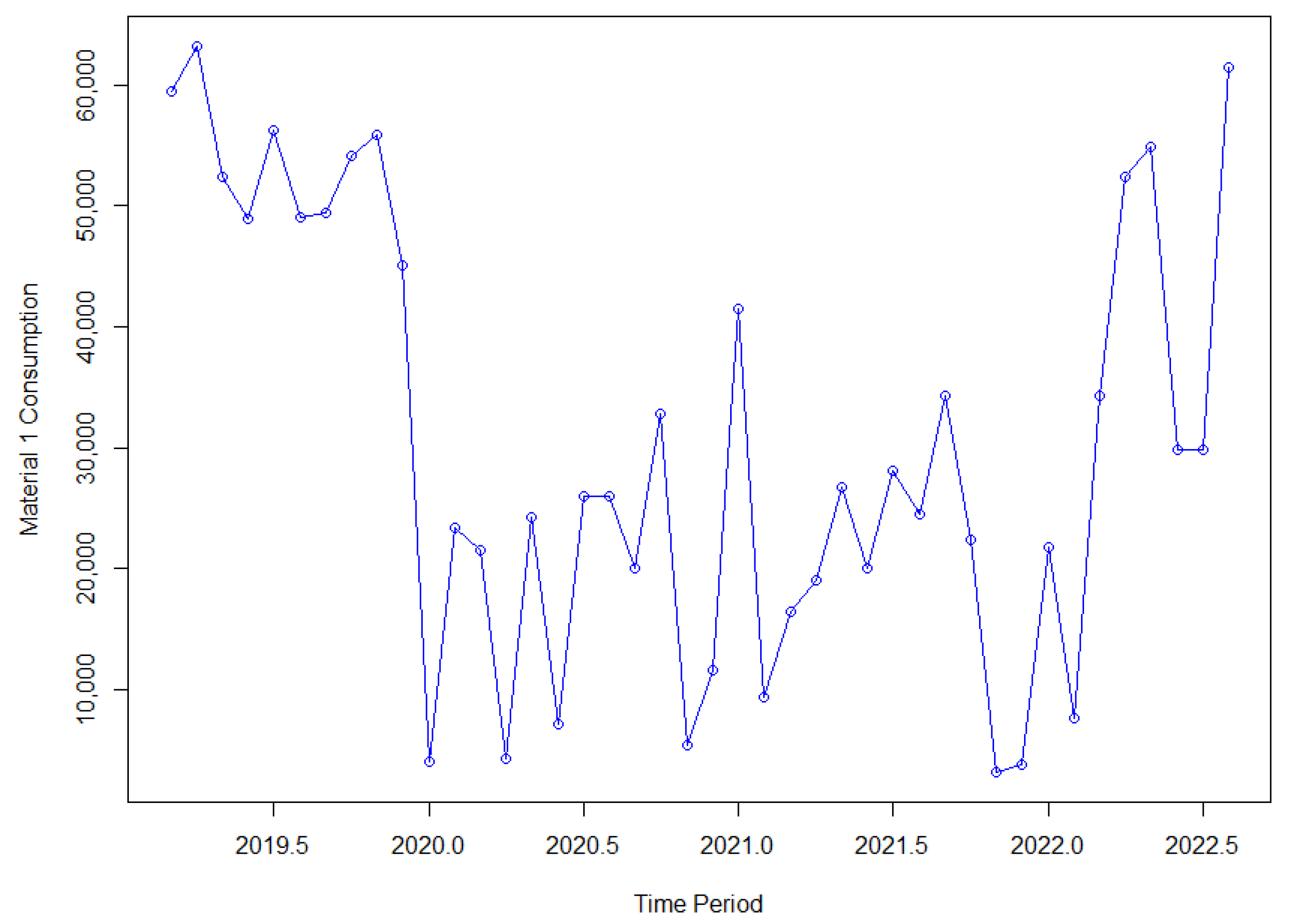
To begin with, it is important to observe the complete time series for the studied material in this work. Figure 1 shows the line chart for all the consumption data (from March 2019 to August 2022), which indicated a significant reduction in consumption towards the end of 2019, followed by a gradual increase from the beginning of 2022. While there could be several hypotheses to explain this phenomenon, such as a change in the product structure via a study of the company’s engineering, this study only focuses on the mathematical analysis and does not delve into any managerial aspects.

To understand the behavior of the series, we analyzed some of the data obtained from descriptive statistics. As shown in the previous Figure, the series did not display any apparent seasonality.

Table 1. Descriptive statistics for Material 1.

Statistics	Value
Minimum	3108
First Quartile	19,261
Median	26,367
Mean	30,507
Third Quartile	49,003
Maximum	63,268
Variance	342,361,647
Standard Deviation	18,503.02
Skewness	0.2
Kurtosis	1.84

presents the descriptive statistics for this series.

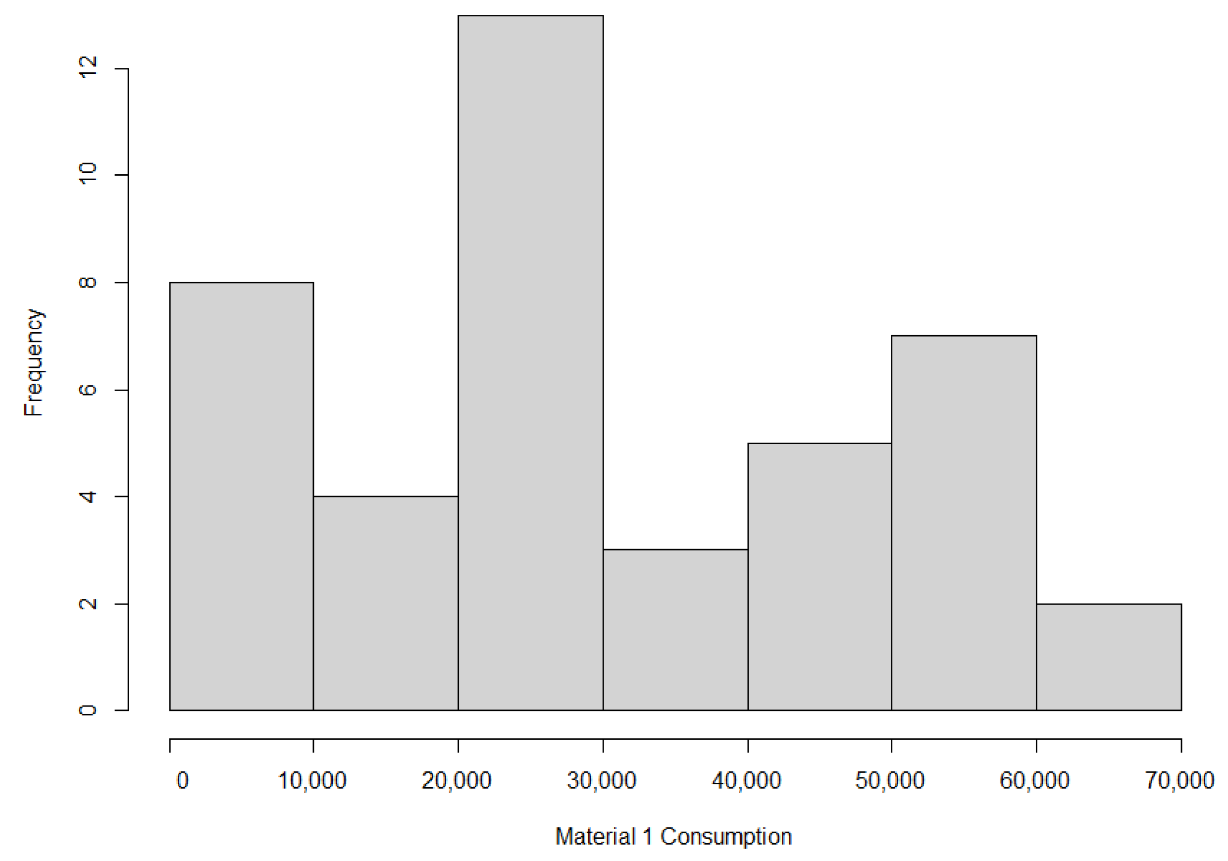
Upon analyzing Table 1, it becomes apparent that Material 1 had a slightly positive skewness, indicating that the right tail of the distribution was slightly longer than the left tail. This was further confirmed by the histogram shown in Figure 2, although it was not easily noticeable by visual inspection. However, the kurtosis value was positive, indicating that the distribution had heavier tails than a normal distribution, which characterizes the flattening or lengthening of the curve. Additionally, Figure 2 highlights that there was a significant concentration of consumption values in the range of 20,000 to 30,000 units.

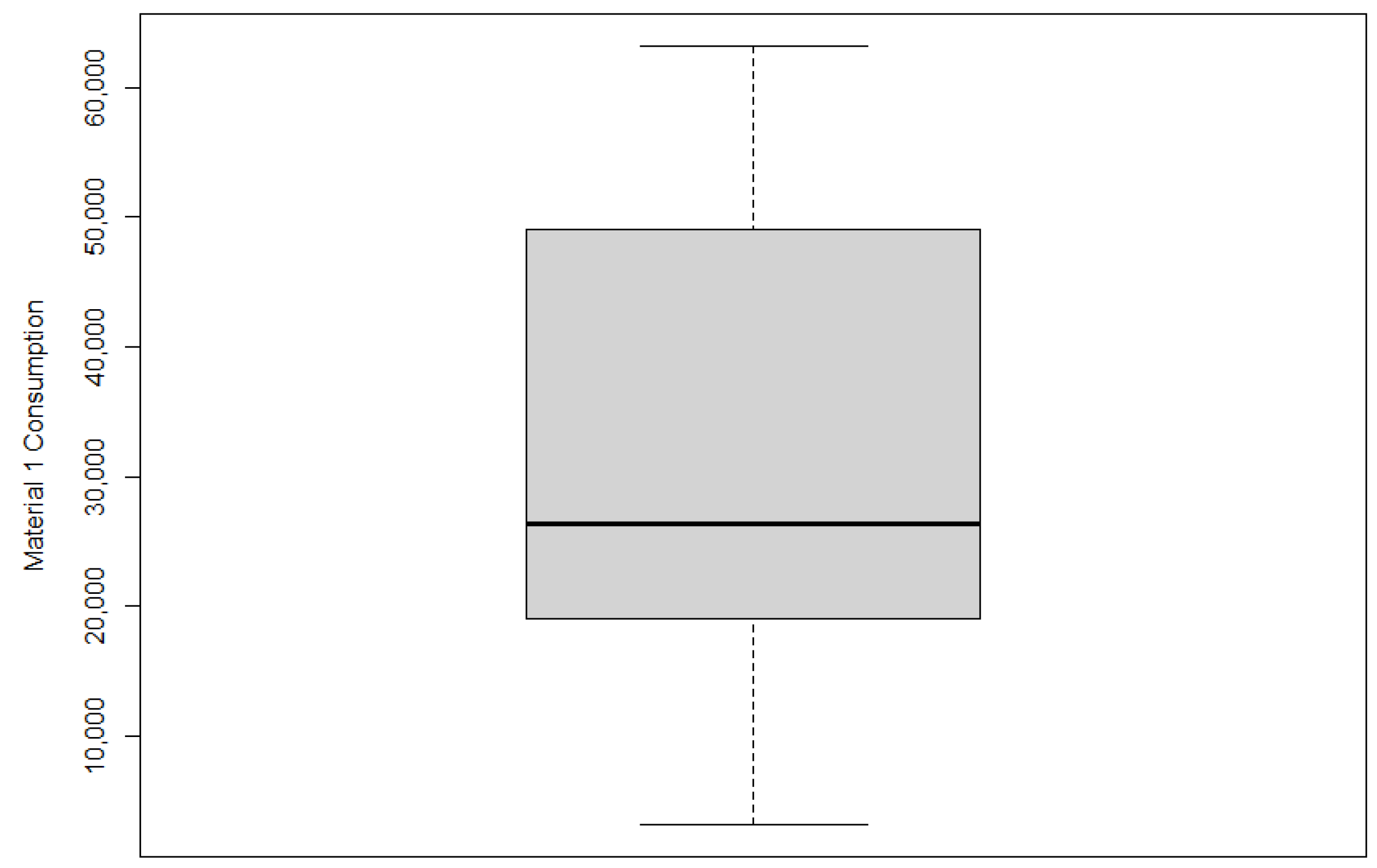
Figure 3 displays a boxplot that can help identify any outliers in the data, which are observations that deviate significantly from the rest of the time series values. It is evident from the plot that the series did not contain any outliers.

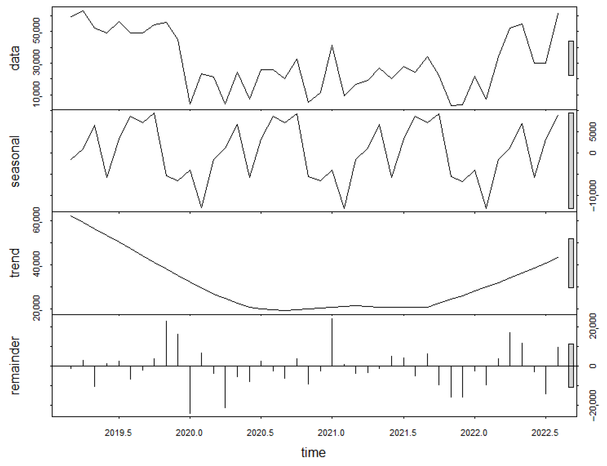
The time series decomposition shown in Figure 4 provides valuable insights into the behavior of the data, where it revealed the absence of seasonality in the series. Furthermore, regarding the trend, as mentioned before, there was a considerable reduction from 2019 onwards, which remained practically stable and only showed an upward trend again from the beginning of 2022, forming an approximate drawing of a negative parabola.

4.1. Forecasting Methods

4.1.1. Simple Exponential Smoothing

The simple exponential smoothing model is a widely used method in demand forecasting and can be used when the sample size is small. The technique is built through a weighted average of past and present values, where exponential weighting assigns greater weights to more recent data and smaller weights to more distant observations [4].

The result of this technique are always constant; in other words, all the forecasts assume the same value, equal to the last level component. This implies that it is appropriate only when the time series does not have a trend or seasonal component [5]. The results of applying this method to the database can be observed in Figure 5.

According to Figure 5, a significant disparity was observed between the actual values of the material 1 time series and the forecasted values for the same period. Hence, the consistent outcomes of the technique were inadequate for the data of this study, as it failed to predict the consumption peak that commenced in March 2022.

4.1.2. Holt

The Holt method, proposed by Holt [6], extends simple exponential smoothing to enable the forecasting of data with a trend. As a result, the forecast values generated by this method are not constant but exhibit a consistent trend (either increasing or decreasing) that extends indefinitely into the future.

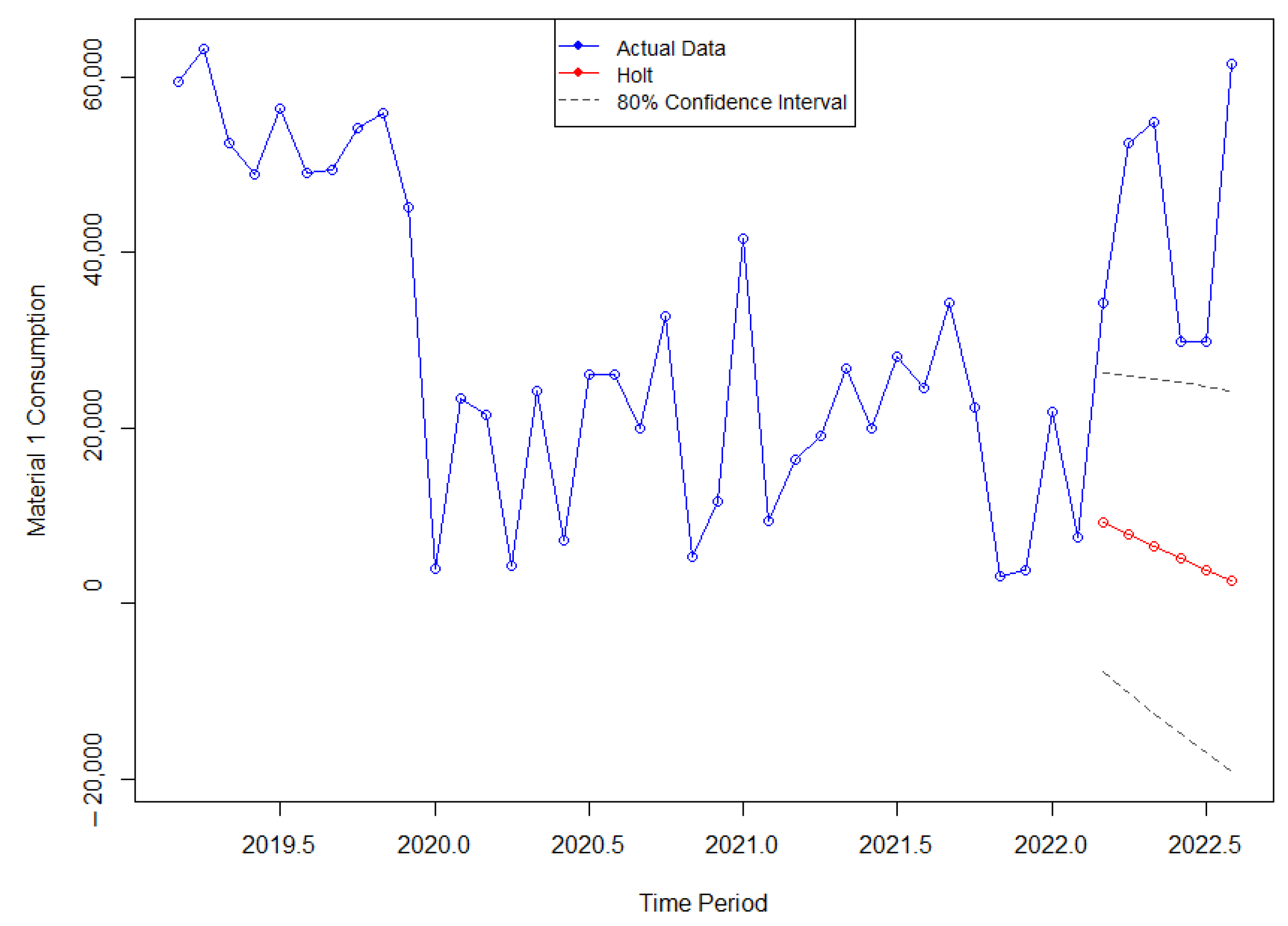
The results of applying this method can be observed in Figure 6 below.

According to Figure 6, there was a significant disparity between the predicted data and the actual consumption values for Material 1. The expected trend should be upward, but the forecast depicted a distinct downward trend. Consequently, this error was substantial enough to conclude that this method was not suitable for this type of time series.

4.1.3. Holt–Winters

The Holt–Winters method is a refined extension of the exponential smoothing approach, where the smoothing procedure provides an overall impression. This method also allows for studying future trends by generating medium and long-term forecasts.

Holt [6] and Winters [7] extended the Holt method to capture the seasonality of a series by proposing two variations that differ in the nature of the seasonal component: additive and multiplicative. Hyndman and Athanasopoulos [5] demonstrated that the additive method is suitable when seasonal variations are relatively constant throughout the series. In this case, the seasonal component is expressed in absolute terms on the scale of the observed series, and in the level equation, the series is seasonally adjusted by subtracting the seasonal component, resulting in an approximately zero sum within each year. On the other hand, the multiplicative method is advised when seasonal variations change proportionally with the level of the series. In this case, the seasonal component is expressed in relative terms (percentages), and the series is seasonally adjusted by dividing it by this seasonal component.

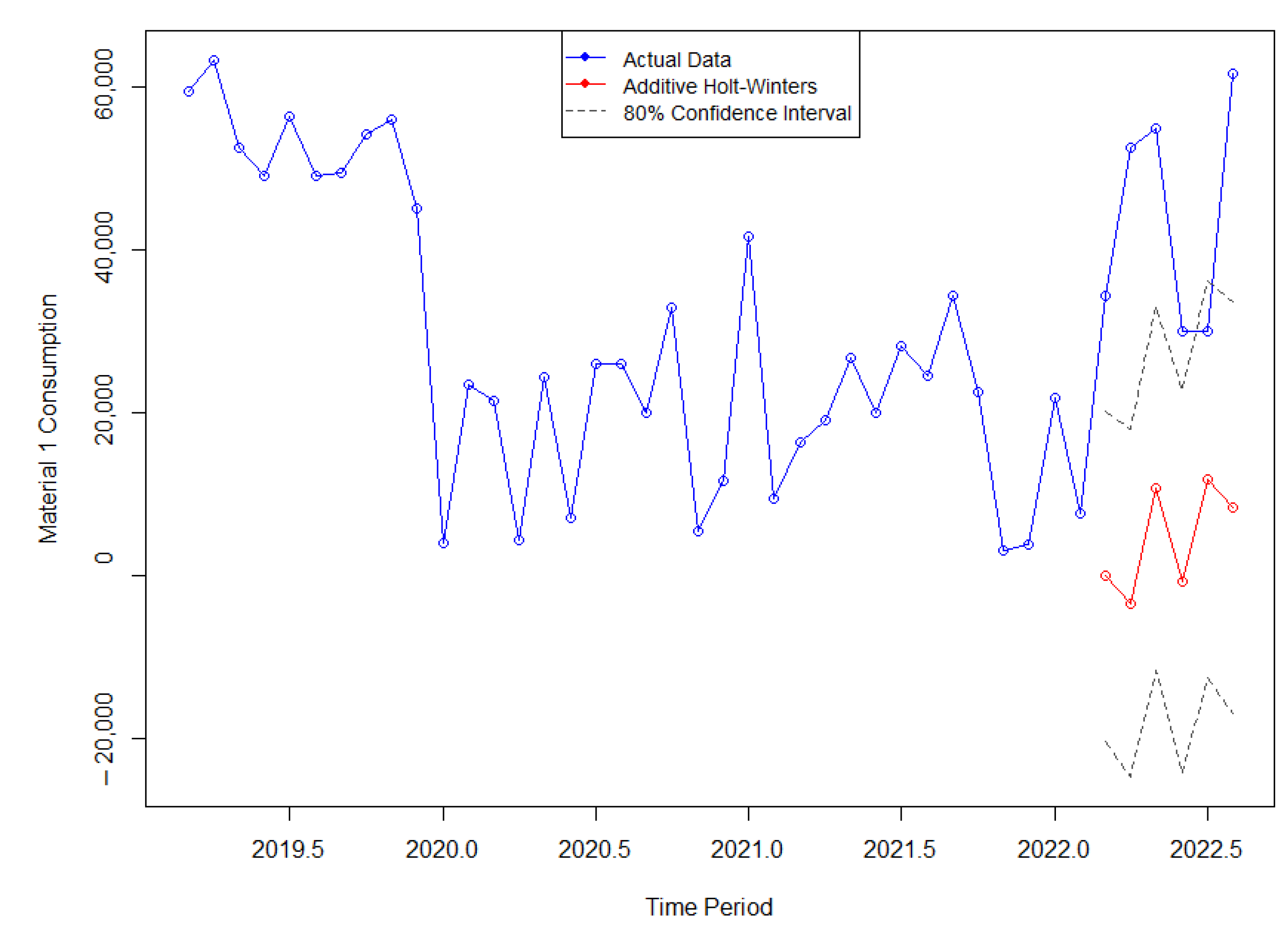
Therefore, beginning with the additive method, the outcomes of applying the Holt–Winters to the Material 1 series are illustrated in Figure 7 below:

By examining the preceding figure, it becomes evident that the method predicted three negative values for the months of March, April, and June 2022. However, such negative values were not feasible in this application. This study employed a real-time series that represented the consumption of a raw material in a production line, and given this context, consumption below zero was not possible. Therefore, it can be concluded that the method was not suitable for the Material 1 series.

Regarding the multiplicative method, while there were no negative values in the forecast for this six-month period, the forecasted trend ended up showing a negative tilt, which contradicted the actual data that exhibited consumption peaks starting from March 2022. This discrepancy in the value relationship can be observed in Figure 8, where due to the multiplication equation employed by the method, the confidence intervals were significantly larger, resulting in a noticeable change in the scale of the line graph.

4.1.4. ETS

Considering the variations in the combinations of trend and seasonality components in the previously mentioned exponential smoothing method, it is possible to use ten new techniques. Each one is labeled by a pair of letters (T and S) that define the type of trend (T) and seasonality (S) components. This classification was first proposed by Pegels [8], who also included a method with a multiplicative trend. It was later extended by Gardner [9] to include methods with an additive damped trend and by Taylor [10] to include methods with a multiplicative damped trend.

The point forecasts generated by the models are identical when the same smoothing parameter values are used. However, they produce different prediction intervals. Additionally, for each method, there can be two models: one with additive errors and another with multiplicative errors. According to Hyndman and Athanasopoulos [5], to differentiate between these two models, a third letter is introduced, denoting the error term. Consequently, each state space model is labeled as ETS (*,*,*) representing (error, trend, seasonality), and this labeling convention can also be interpreted as exponential smoothing. Each combination of components has its own set of equations, and the possibilities for each component are as follows: Error = A, M; Trend = N, A, Ad; and Seasonality = N, A, M. In this context, A represents additive, M represents multiplicative, N represents none, and Ad represents additive damped.

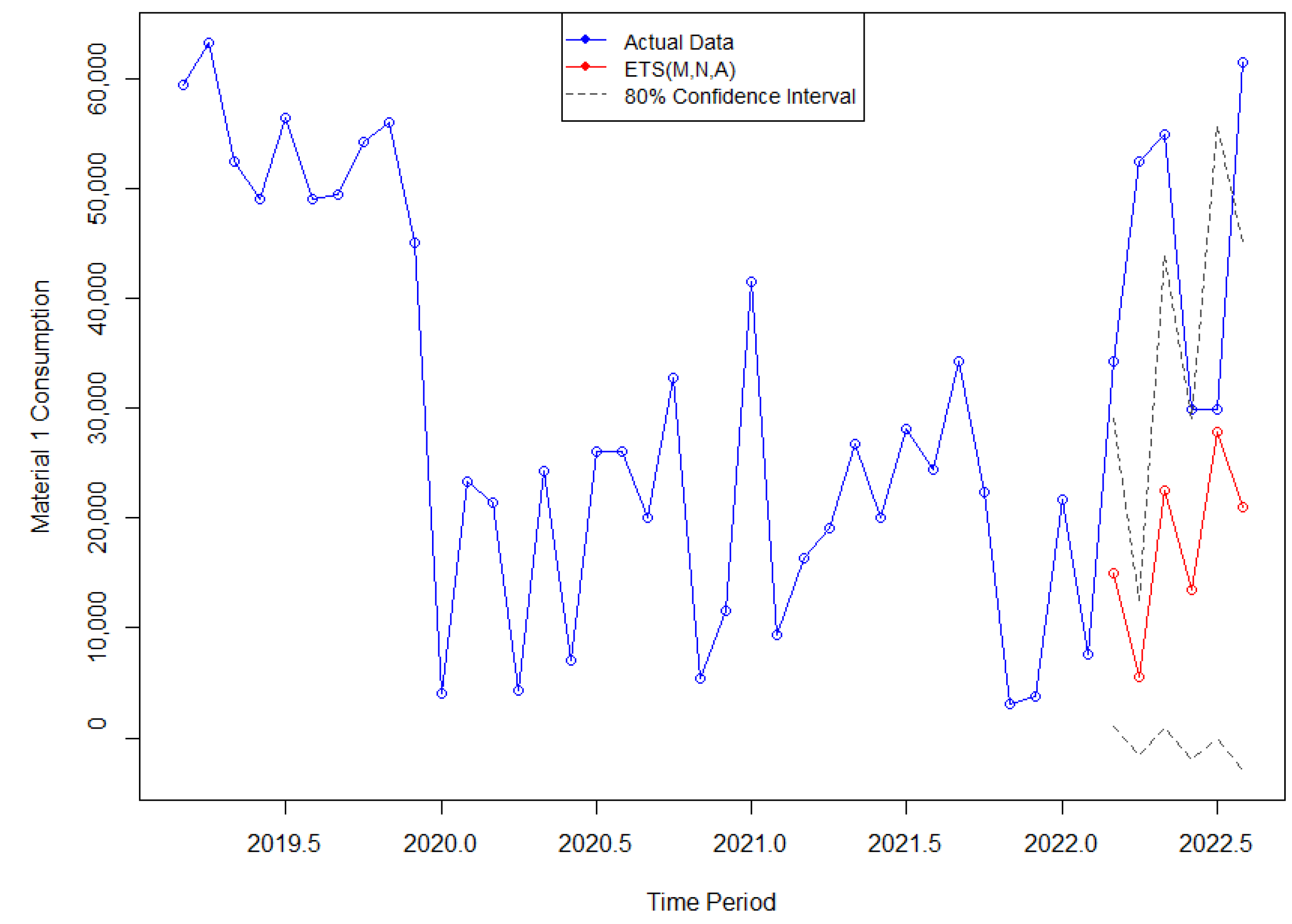
In this study, all the possible label combinations were tested, and the root mean square error (RMSE) was measured for each combination by comparing the predicted data with the actual data. The model with the lowest RMSE was selected, which happened to be the ETS (M,N,A): multiplicative error, no trend, and additive seasonality. The computed results of this method can be observed in Figure 9.

Upon comparing the predicted data generated by the ETS (M,N,A) method with the actual consumption values for the corresponding period, it is apparent that the technique accurately forecasted a positive trend, distinguishing itself from certain previous methods. Nevertheless, there remained a notable disparity in the magnitude of the peaks.

4.1.5. Naïve

The Naïve model is one of the simplest methods for time series forecasting and works well for many economic sectors and financial time series. The Naïve Simple technique involves using the exact value of the last observation in the time series as the forecast, but some variations take into consideration the seasonality and are referred to as Seasonal Naïve. In this case, the forecast is based on the same observed value from a previous point in the same season, such as the value from the same month but in the previous year [5].

The model used in this work is the Seasonal Naïve method, considering the forecast value of the same month from the previous year in the time series. Figure 10 depicts the graph of the results obtained by applying this model.

Upon examining the forecast graph generated by the Naïve method and comparing it with the actual data, several noteworthy observations come to light. While this method demonstrated limitations in accurately predicting the extreme peaks observed in four particular months, it showcased exceptional accuracy during the months of June and July, closely aligning with the actual data and capturing the upward trend exhibited by the data. These findings suggest that the Naïve method exhibits potential for capturing seasonality in specific months, albeit with limitations in predicting extreme fluctuations.

4.1.6. ARIMA

The designation of the ARIMA model stands for Autoregressive Integrated Moving Average and refers to a type of self-regressive model that allows for predicting the values of a variable based on its previous values without the need for other auxiliary information or related variables [11]. The generic name ARIMA for these models refers to their three main components: Autoregressive (AR), Integrated (I), and Moving Average (MA). In these models, the aim is to describe autocorrelations in the data, where each observation of a variable at a given time is modeled based on previous values over time for the same variable.

In this approach, the modeling process involves deriving an ARIMA model that fits the given dataset, which requires analyzing the essential characteristics of the time series, such as trend, seasonality, cyclical variations, autocorrelation functions, and residuals [5]. Another point is that for the application of the model, the time series must necessarily be stationary, meaning that their statistical properties remain constant over time. If they are not stationary, it will be necessary to differentiate the data until they become stationary.

The initial step of the ARIMA model involved applying a logarithmic transformation to the data and subsequently differencing them to achieve stationarity. In the case of the time series of Material 1, it was only necessary to difference it once to achieve stationarity. To confirm this, the Dickey–Fuller unit root test was used.

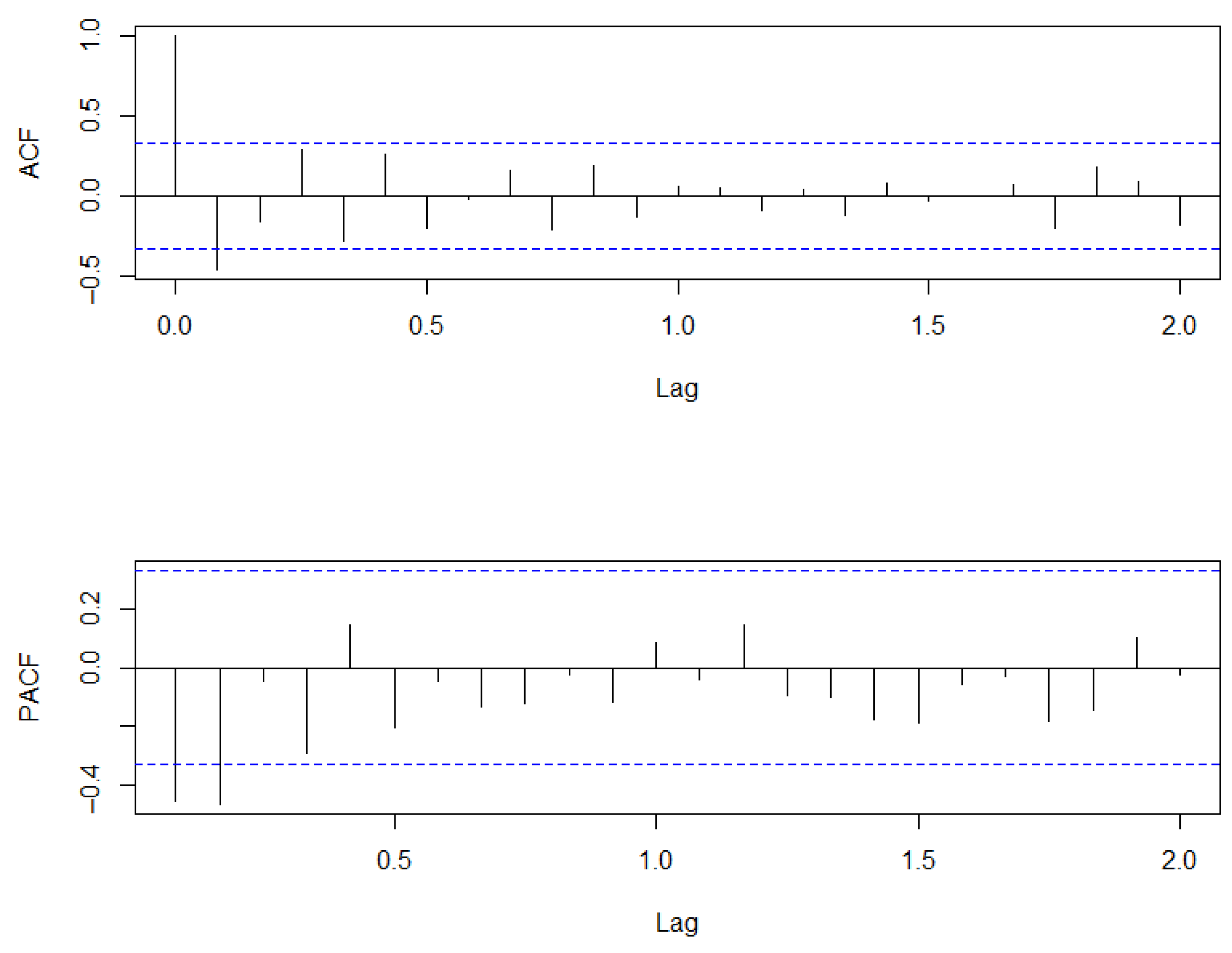
Consequently, to proceed with the application of the method, it was necessary to identify the model using the autocorrelation function (ACF) for the “MA” term and the partial autocorrelation function (PACF) for the “AR” term. Both were applied to the differenced time series and can be analyzed in Figure 11.

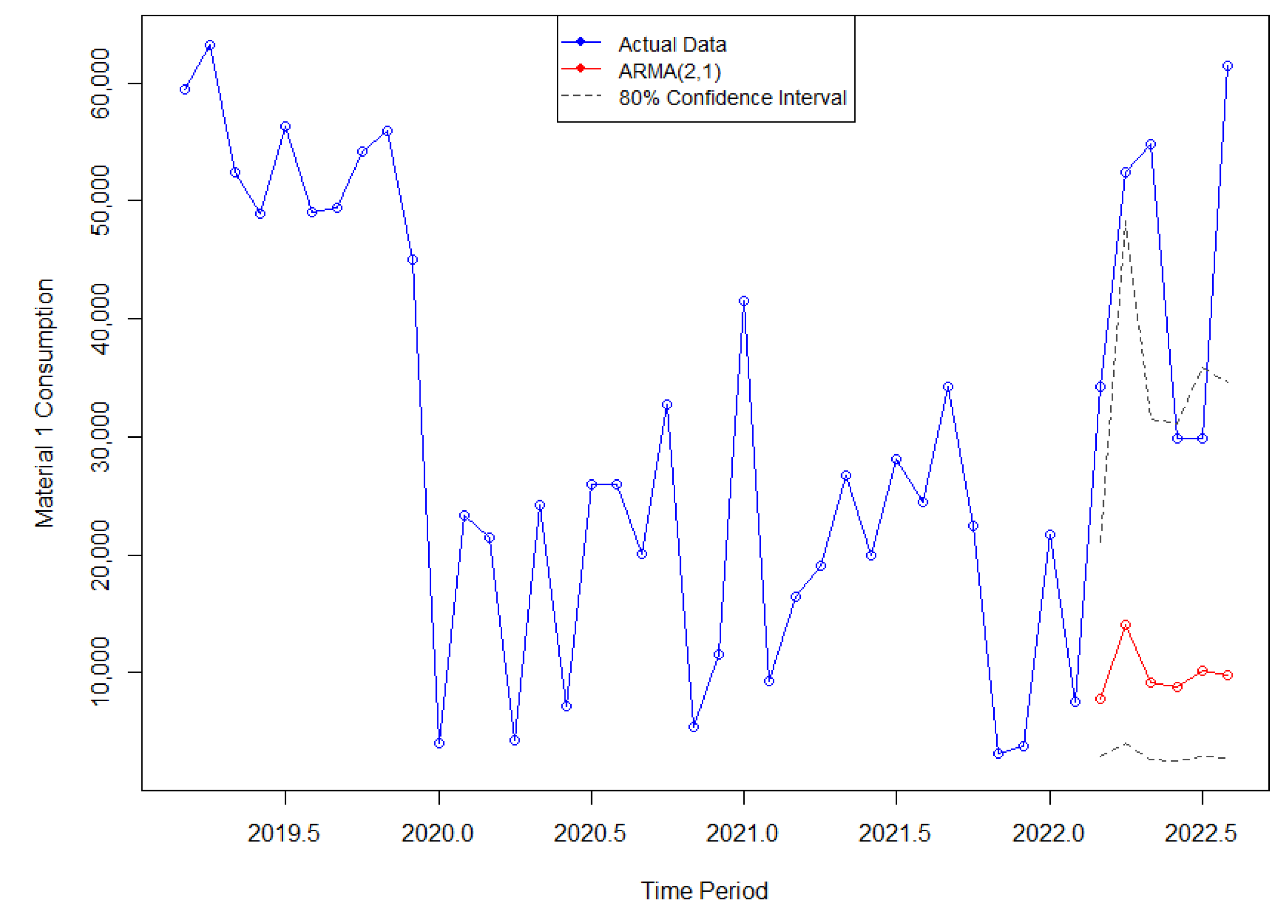
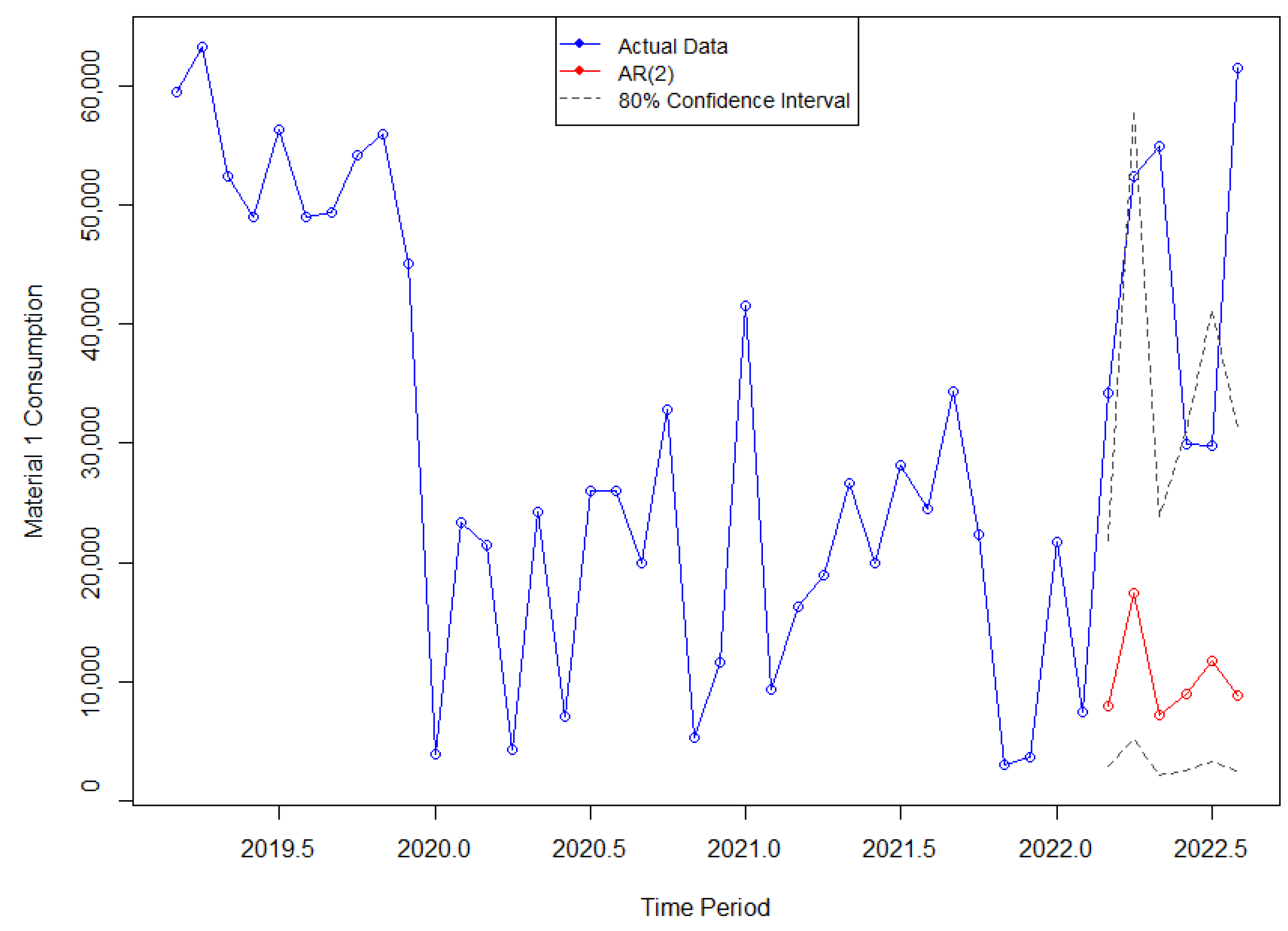
Based on these analyses, several combinations for the method can be considered. The chosen models were the ARMA(p = 2, d = 0, q = 1) and the AR(p = 2, d = 0, q = 0). Subsequently, the forecasts generated by both the ARMA(2,1) and AR(2) models for the Material 1 time series did not capture a significant peak in March 2022, in contrast to the actual value of the series, which was considerably higher. However, the confidence intervals were able to approximate the substantial increase in values from that period onwards, which some of the previously mentioned methods failed to capture. A visual comparison between the actual data and the generated forecasts can be observed in Figure 12 and Figure 13.

4.1.7. Neural Network

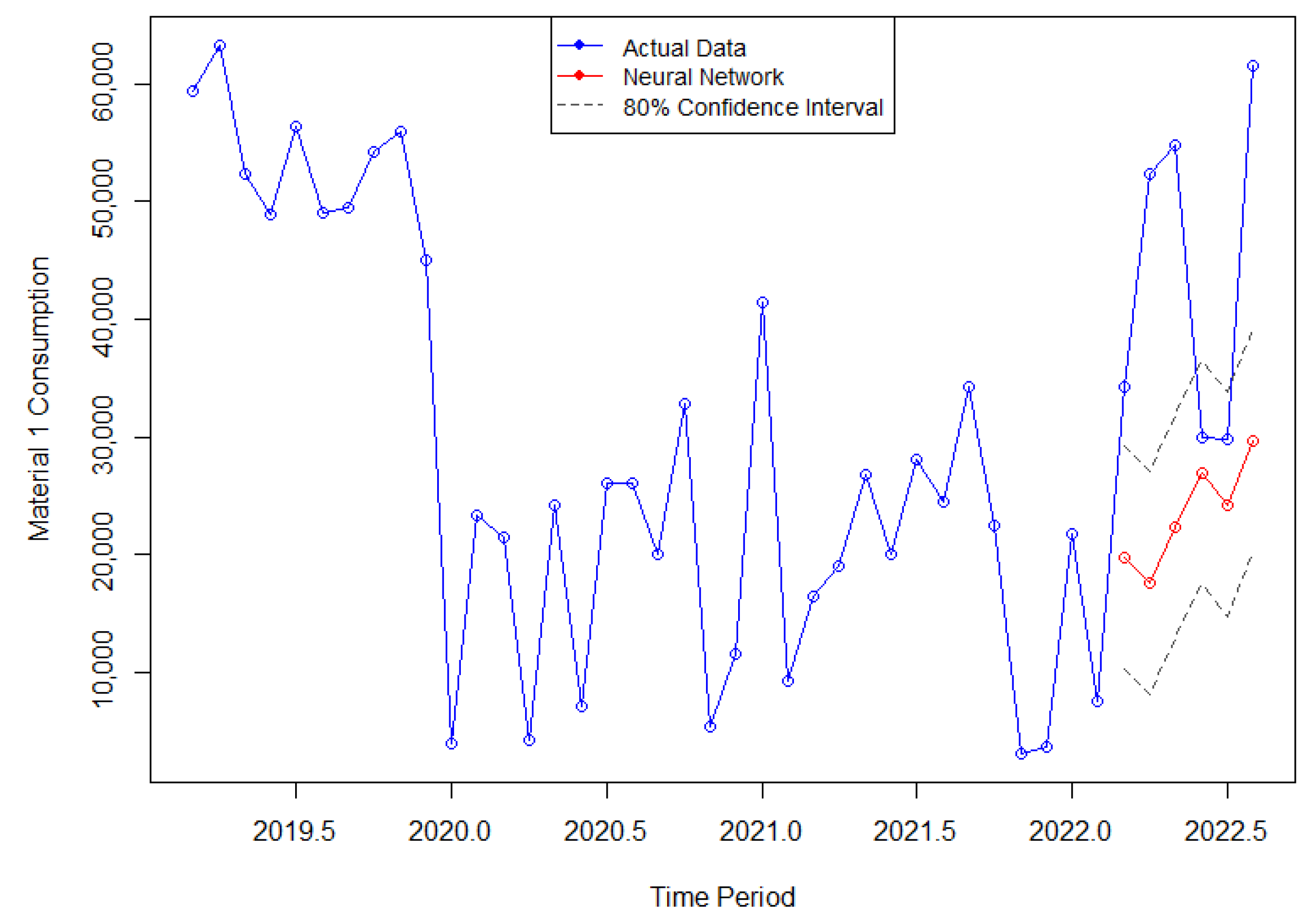
The final technique applied in this study was the neural network, based on the autoregression with neural networks (AR-NN) approach that combines autoregression (AR) and neural networks (NN) techniques to model time series. The results obtained with this technique are presented in Figure 14.

The analysis of the forecast graph generated by the neural network reveals several noteworthy observations. Firstly, the method successfully captured and predicted a positive trend that aligned reasonably well with the actual data. However, it showed limitations in accurately predicting the highest peaks of the data, which suggests potential challenges in capturing extreme fluctuations. Despite this, it is important to highlight the remarkable performance of the forecast during the months of June and July, where during these months, the predicted data closely aligned with the actual data, indicating a high level of accuracy and precision during that specific period. These findings demonstrate the model’s ability to capture and replicate patterns effectively, particularly during months characterized by more stable and predictable trends.

4.2. Evaluation Metrics

To determine the best-performing forecasting method among those presented, it was necessary to measure the errors by comparing the actual data with the predicted data. Therefore, this study employed three different metrics to analyze the effectiveness of the techniques: the Symmetric Mean Absolute Percentage Error (sMAPE), Theil’s U Index of Inequality, and the Root Mean Square Error (RMSE).

The Symmetric Mean Absolute Percentage Error (sMAPE) was proposed by Makridakis [12] in order to correct some disadvantages; that is, a modified Mean Absolute Percentage Error (MAPE) has a heavier penalty for forecasts that exceed the actual than those that are less than the actual. So, this metric is a modified MAPE, in which the divisor is half of the sum of the actual and forecast values.

The Theil’s U Index of Inequality is an accuracy measure often cited in the literature, and according to Bliemel [13], there is confusion about this index, which may result from the fact that Theil [14] proposed two distinct formulas, but with the same name. The first proposal is bounded between 0 and 1, and this metric is used in this study. In the second proposal, the upper limit is infinite. This metric analyzes the quality of forecasts, and the closer it is to zero, the lower the prediction error generated by a specific model. In other words, it indicates that a forecast is better than the trivial forecast [15].

The Root Mean Square Error (RMSE) is calculated as the square root of the mean of the square of all of the error. It is widely used and considered an excellent general-purpose error metric for numerical predictions. The RMSE provides a reliable measure of accuracy, particularly when comparing forecasting errors among different models or model configurations for a specific variable. However, it should be noted that the RMSE is scale-dependent and cannot be directly compared between variables [16].

In

Table 2. Evaluation metrics for Material 1.

Forecasting Method	sMAPE	Theil’s U Index of Inequality	RMSE
Simple Exponential Smoothing	1.094186	0.7519919	34,314.91
Holt	1.500099	0.8816619	40,232.01
Holt–Winters Additive	1.623714	0.9098164	41,516.76
Holt–Winters Multiplicative	1.559045	0.8978318	40,969.88
ETS(M,N,A)	0.8413673	0.6653724	30,362.28
Naïve	0.6081907	0.5440008	24,823.86
ARMA(2,1)	1.230298	0.7892819	36,016.53
AR(2)	1.203849	0.7858103	35,858.11
Neural Network	0.5643272	0.5319228	24,272.71

, it is possible to observe the three mentioned metrics for each of the nine forecasting methods.

After examining the table above, it becomes evident that the Holt–Winters methods, both additive and multiplicative, yielded the highest error measurements. This indicates that these particular methods were less effective in accurately forecasting the given time series. Similarly, Holt’s method and the combinations of the ARIMA, such as the ARMA(2,1) and AR(2), exhibited high error metrics, further suggesting their inefficiency in this context. Surprisingly, the simple exponential smoothing method, despite its simplicity and constant forecasting values, outperformed more complex approaches such as the ARIMA models. The top three performing methods, ranked in order, were the Neural Network, Naïve, and ETS (M,N,A). These findings highlight the importance of selecting the appropriate forecasting techniques tailored to the characteristics of the specific time series at hand. In the following section, conclusions are drawn based on these results and potential avenues for future research are discussed.

5. Discussion

The obtained results provide valuable insights into the performance of different forecasting methods in the context of the analyzed time series. The observed high error measurements for the Holt–Winters methods, both additive and multiplicative, suggest that these approaches may not be well-suited for capturing the underlying patterns and dynamics of the given time series. Similarly, the relatively high error metrics observed for Holt’s method, ARMA(2,1), and AR(2) indicate their suboptimal performance in capturing the complexities of the analyzed time series. These methods, although widely used, rely on assumptions that might not hold true for every type of time series. Consequently, alternative approaches should be considered for improved forecasting accuracy in similar contexts.

Remarkably, the simple exponential smoothing method exhibited better performance compared to the more complex models. Despite its straightforward nature and constant forecasting values, it demonstrated competitive accuracy in predicting the examined time series. This finding aligns with Makridakis et al.’s [17] study that emphasized the effectiveness of simple methods, which often produced more accurate forecasts compared to complex approaches like ARIMA models.

The top three performing methods, namely the Neural Network, Naïve, and ETS (M,N,A), merit further attention. The ETS ((M,N,A), based on exponential smoothing, incorporates multiple components such as error, trend, and seasonality, and has been successfully applied to various time series forecasting problems. Naïve forecasting, although simplistic in its approach, often serves as a benchmark against which more sophisticated methods are evaluated. Its competitive performance in this study suggests that even basic forecasting strategies can yield accurate results under certain conditions. Finally, the Neural Network approach, known for its ability to capture nonlinear relationships and complex patterns, displayed promising results, indicating its potential for accurate time series forecasting.

From a broader perspective, these findings underscore the significance of comprehending the characteristics and dynamics of the specific time series when choosing an appropriate forecasting method. In the context of this study, the time series exhibited high volatility, posing challenges for accurate forecasting. Consequently, no single method emerged as universally superior in all scenarios, highlighting the imperative nature of meticulous evaluation and comparison of diverse techniques.

Future research directions in time series forecasting may include investigating the effectiveness methods that combine the strengths of multiple forecasting techniques, exploring hybrid approaches that integrate machine learning and statistical modeling, and considering also the impact of external factors on the forecasting accuracy.

In conclusion, this study offers valuable insights into the performance of various forecasting methods, with implications for practitioners and researchers in the field of time series analysis, particularly in the context of the aeronautical industry, where raw materials play a vital role. The findings highlight the significance of selecting the most suitable method, as even a slight difference in forecasting error can lead to substantial cost savings when planning and procuring essential inputs. By leveraging these findings and considering the suggested future research directions, it becomes feasible to enhance forecasting capabilities and make significant contributions to the advancement of the field of time series forecasting.