Abstract
Water resource forecasting plays a crucial role in managing hydrological reservoirs, supporting operational decisions ranging from the economy to energy. In recent years, machine learning-based models, including sequential models such as Long Short-Term Memory (LSTM) networks, have been widely employed to address this task. Despite the significant interest in forecasting hydrological series, weather’s nonlinear and stochastic nature hampers the development of accurate prediction models. This work proposes a Variational Gaussian Process-based forecasting methodology for multiple outputs, termed MOVGP, that provides a probabilistic framework to capture the prediction uncertainty. The case study focuses on the Useful Volume and the Streamflow Contributions from 23 reservoirs in Colombia. The results demonstrate that MOVGP models outperform classical LSTM and linear models in predicting several horizons, with the added advantage of offering a predictive distribution.
1. Introduction
Hydrological forecasting plays a crucial role in planning and operation activities. On a short-term scale, it allows for management of water systems and resources, including irrigation, flood control, and hydropower generation. In the energy sector, hydrological forecasting supports the optimal scheduling of hydroelectric power generation. Accurately predicting hydroelectric plants’ water release and reservoir volume enables scheduling optimal thermal plant generation while minimizing fuel costs and improving the energy sector’s sustainability [1,2]. For example, Brazil’s National Electrical System Operator provides streamflow time series of hydropower plants that supports forecasting research [3]. In Colombia, hydropower plants contribute 97.37% of the renewable energy, including 87.54% from reservoirs [4]. Therefore, there is a great interest in developing accurate hydrological forecasting models to manage and exploit water resources sustainably and effectively.
Forecasting models can be short-, mid-, or long-term, where the former enable dispatch and optimization for power systems. Long-term forecasting supports reliability planning through system expansions and weather analysis at a large scale [5,6]. Hence, the design of forecasting models depends on the prediction horizon, with two primary approaches: physically-driven concept rules and data-driven models which learn from time-series samples. Models in the first category have demonstrated their capability to predict various flooding scenarios. However, physical modeling often requires extensive knowledge and expertise in hydrological parameters and various datasets, demanding intensive computation which results in unsuitability for short-term prediction [7]. Since data-driven models can learn complex behavior from the data, streamflow forecasting traditionally relies on this second approach. The most extensively used data-driven forecasting model is the Linear AutoRegression (LAR), due to its simplicity and interoperability [8]. However, LAR fails to adequately represent streamflow series because of the complex water resource patterns, such as varying time dependencies, randomness, and nonlinearity [3,6,9].
The most prominent models for dealing with nonlinear trends are neural networks (NNs), known for their flexibility and outperformance of other nonlinear models [10]. For instance, a hybrid model coupling extreme gradient boosting to NNs predicted monthly streamflow at Cuntan and Hankou stations on the Yangtze River, outperforming baseline support vector machines [11]. Additionally, recurrent architectures, such as Long Short-Time Memory (LSTM), have proven to improve the scores of classical NNs in daily streamflow forecasting, given their ability to capture seasonality and stochasticity [5,8]. However, the numerous neural network architectures available make researchers question which one will best fit a given problem, as no single model is universally applicable [7]. Further, the inherent noise present in hydrological time series influences forecasting accuracy [3,10].
Some operational tasks demand uncertainty quantification for the prediction due to the inherent noise. Gaussian Processes (GP) satisfy such a requirement by approximating a predictive distribution. GP-based forecasting has proven remarkable results in streamflow forecasting up to one day and month ahead [12,13]. In addition, a kernel function, combining squared exponential, periodic, and rational quadratic terms, allowed GP models to fit streamflow time series for the Jinsha River [9]. In another approach, a probabilistic LSTM coupled with a heteroscedastic GP produced prediction intervals without any post-processing to manage the daily streamflow time series uncertainty [14]. However, GP-based approaches pose two research gaps [15]. Firstly, the probabilistic couple approach still complicates the model calibration. Secondly, natural probabilistic modes such as GP have only been used to study scalar value signals.
This work develops a forecasting methodology using a GP-based probabilistic approach applied to hydrological resources, supporting multiple output predictions and reducing the model training complexity. The methodology, termed MOVGP, combines the advantages of Multi-Output and Variational GPs for taking advantage of relationships among time series, adapting the individual variability to handle large amounts of samples. The research compares the performance of the MOVGP against an LSTM neural network and a Linear AutoRegression (LAR) model in forecasting two multi-output hydrological time series, namely, Useful Volume and Streamflow Contributions of 23 reservoirs. It is worth noting that the considered time series correspond to actual reservoir data taken into account for hydropower generation in Colombia. Attained results prove the ability of MOVGP to be adapted to varying prediction horizons, generally outperforming contrasted models.
The paper agenda is as follows: Section 2 covers methodologies and theoretical bases used for developing and training Multi-Output Variational GP models; Section 3 validates the MOVGP training and tests the three models in terms of the Mean Square Error (MSE); Final remarks and future work conclude the work in Section 4.
2. Mathematical Framework
2.1. Gaussian Process Modeling Framework
A Gaussian Process (GP) is a collection of random variables related to the infinite-dimensional setting of a joint Gaussian distribution. Consider the dataset of N samples , where is the design matrix, with columns of vector inputs of L features, and is the target matrix, with columns of vector outputs of D outputs for all N cases. GP framework conditions a subset of observations to create a map that models the relationship between to .
Then, the Single-Output GP (SOGP) attempts to represent a scalar-valued function , i.e., where with GP framework. This model is completely specified by a mean function and covariance (kernel) function , with vector parameters and notated, respectively, as follows:
In more realistic scenarios, single-output observation y presents Gaussian noise models as a noise-added version of the function f, such as . Let be a test matrix with test vector inputs , , in which denotes mean train vector, denotes mean test vector, denotes covariance train matrix, denotes covariance train–test matrix, and denotes covariance test matrix. The joint Gaussian distribution of the observations vector and test outputs vector , named previously, are specified as shown:
where is the identity matrix of size N derived in the conditional distribution, calculated as follows:
with the following definitions:
Notice, from Equations (4) and (5), that mapping construction is analytic and, therefore, does not employ an optimization process. Nevertheless, selection of parameters at and and observation noise variance can be estimated using marginal likelihood from Equation (2), , and minimizing negative log marginal likelihood:
where is the covariance matrix for the noisy observations. Thus, the optimization problem in Equation (6) can be efficiently solved via a gradient-based optimizer [16].
2.2. Multi-Output Gaussian Process (MOGP)
MOGP generalizes SOGP mapping for outputs as with GP framework, where is a vector-valued function. The MOGP model, similar to the SOGP model, is entirely defined by its mean vector function and covariance matrix function , each with vector parameters and , respectively, expressed as follows:
Let be a diagonal matrix such that , with being the output observation noise variance and being a ravel version vector of target matrix . Following the procedure established in Equation (3), deriving the MOGP posterior distribution takes place as follows:
with the following definitions:
where , ⊗ represents the Kronecker product between matrices and upper index D denotes version of SOGP quantities.
To deal with developing an admissible correlation between outputs, the Linear Model of Coregionalization takes place, expressing each output of MOGP as a linear combination of Q (known as latent dimension) independent SOGP as follows:
where is the vector coefficients, with values associated with contributions of the q-th independent SOGP at the output with kernel function . In this way, the covariance matrix of the MOGP model is given by the following [17,18]:
where is a semi-definite positive matrix known as the coregionalization matrix.
2.3. Variational Gaussian Process (VGP)
The main challenge in implementing MOGP models lies in their complexity and storage demand becoming intractable for a dataset of a few thousand samples [19], because the need to invert the matrix in Equations (9) and (10) is usually performed by Cholesky decomposition. To overcome the problem of computational complexity, a new set of trainable inducing points and inducing variables augment the output variables . The marginal distribution for the output variables is expressed as . The Variational Gaussian Process (VGP) allows approximating with by marginalizing out the set of inducing points [20]:
Since the output distribution comes from a MOGP, is assumed as Gaussian , with mean and covariance , so that the approximating distribution also becomes Gaussian:
with , as the kernel function in Equation (12) evaluated at all pairs of inducing–training points and the kernel function values between pairs of inducing points. Since optimizing the parameters of yields a stochastic framework, the cost function in Equation (6) turns into a tractable marginal likelihood bound for the multi-output case:
in which is the Kullback–Leibler (KL) divergence between and . This approach offers a notable benefit by diminishing the complexity of the MOGP to due to the inversion of the matrix , which is smaller than . As a result, the model can efficiently handle an increased number of samples N, providing an opportunity to gather more information from the dataset at a reduced cost.
3. Results and Discussions
The current section aims to thoroughly communicate the implications of the forecasting results on hydric time series using MOVGP. Firstly, we offer a detailed description of the considered dataset, including information on its sources, characteristics, and preprocessing steps. Further, the manuscript details the hyperparameter tuning experiments and describes the validation strategy. Finally, we examine the forecasting performance and highlight notable trends and observations.
3.1. Dataset Collection
We validate the MOVGP regressor on a hydrological time series forecasting task of the Useful Volume and Contributions from 23 Colombian reservoirs, daily recorded daily from 1 January 2010, to 28 February 2022, yielding 4442 daily measurements. Despite the volumetric nature of the raw data, the hydroelectric power plants report Useful Volumes and Streamflow Contributions as their equivalent in kilowatt-hour (kWh) units, since such a representation is more practical for daily operations. Figure 1 visually describes the statistics for each reservoir. Note that amplitudes vary from millions to billions of kWh among reservoirs, due to each generating at a different capacity. In the case of Useful Volumes, one finds some highly averaging time series with a few variations (see reservoirs A and L), but also cases of low means with a significant variation (as the reservoir B). Notice from Streamflow Contributions that the reservoir K boxplot does not appear, due to zero values reported for all time series. Some reservoirs also present outlier volume reductions (black crosses), contrasting with the outlier increments in streamflow. Two main factors produce the above nonstationary and non-Gaussian behavior: the Colombian weather conditions produce unusual rainy days and long dry seasons, and the operation decisions can impose water saving or generation at total capacity each day.
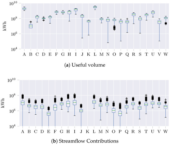
Figure 1.
Time series distributions of Useful Volume and Streamflow Contribution for each reservoir on the dataset. Amplitude axis is presented in logarithmic mode due to large scale variations.
3.2. MOVGP Setup and Hyperparameter Tuning
Firstly, we define the validation task as predicting the H-th day in the future using the current hydrological measurement in all the reservoirs, yielding inputs. Prediction horizon H ranges from one to twenty-five days, exploring short- and medium-term hydrological forecasting performance. For proper validation, MOVGP and contrasting approaches were trained on the first 10 years and validated on the data from 28 February 2021 to 28 February 2022, corresponding to 365 testing samples. Figure 2 presents the testing time series for the Useful Volume of three reservoirs. Noting the varying scales that lead to potential bias during the training stage, a preprocessing step normalizes the dataset by centering the time series from each reservoir on zero and scaling it to unit standard deviation. Normalizing means and standard deviations result from the training subset statistics avoids test biasing.
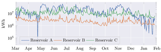
Figure 2.
Testing data for Streamflow Contributions of three reservoirs from March 2021 to February 2022, evidencing the within and between time series variability.
Each type of time series, Useful Volume and Streamflow Contribution, considers an individual forecasting model. Hence, the experimental framework trains two independent MOVGPs with outputs. The proposed methodology considers a constant for the MOVGP mean function, , with as the single trainable vector parameter. The proposed methodology builds the MOVGP covariance function in Equation (12) from the widely used squared exponential, in Equation (16), allowing a smooth data mapping:
where the diagonal matrix gathers the length scale factors from each input dimension. The trainable covariance parameters become and from the Q independent SOGP within the MOVGP framework. Then, a 10-fold time series split model selection determines the optimal hyperparameter setting for the forecasting models by searching within the following grid: number of inducing variables and latent space dimension .
Figure 3 presents the 10-fold-averaged cross-validation mean squared error (MSE) along the grid search while fixing the model horizon to for both the Useful Volume and Streamflow Contributions. Hyperparameter tuning exhibits that, the larger the Q and M, the smaller the MOVGP error and the slower the improvement. Therefore, the forecast task on a very short horizon yields complex models that hardly overfit. However, the latent dimension influences the performance significantly more than the induced variables, agreeing with the model development: the latent dimension controls the embedding quality, while the induced variables reduce the computational burden without compromising the performance.
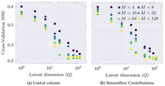
Figure 3.
MOVGP hyperparameter tuning for horizon using a grid search on the latent space dimension L and the number of induced variables M. Testing MSE is computed on a 10-fold cross-validation.
For each considered horizon , Figure 4 illustrates the hyperparameters which reach the best testing MSE. For the Useful Volume time series, shown in Figure 4a, the number of latent variables Q increases while the number of inducing points M decreases. A Pearson correlation coefficient of between the optimal Q and M indicates that the model trades off its complexity between hyperparameters: increasing Q allows a more flexible model, whereas increasing M produces MOVGP models that retain more information about the time series. In turn, the optimal Q for the Streamflow Contribution remains at the highest evaluated value while M decreases for the last horizons (Figure 4b). Such a fact suggests that the latent space is large enough to decode the relationship between past Streamflow Contributions and the farthest horizon. Thus, a flexible model evades a large explicit memory to seize the relevant dynamics, and vice versa.
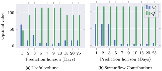
Figure 4.
Optimal MOVGP hyperparameters, according to the testing MSE along the prediction horizon H for Useful Volume and Streamflow Contributions.
3.3. Performance Analysis
The performance analysis compares MOVGP against two widely considered hydrological forecasting models: a straightforward Linear AutoRegression (LAR) model as a baseline and a Long Short-Term Memory (LSTM) network with the hidden space dimension and the number of recurrent layers as hyperparameters. Specifically for the LSTM, the same model selection strategy—10-fold time series split—tunes the hyperparameters using the training subset. Figure 5 illustrates the MSE for the 10-fold cross-validation attained by the three contrasted models along the explored horizons for both time series. In general, error increases with the prediction horizon, due to the forecasting task becoming more complex for far away days. Nonetheless, the autoregressive model outperforms LSTM, closely followed by MOVGP, up to a 15-day horizon, suggesting linearly-captured time dependencies in the short term. In contrast, MOVGP reaches the lowest error for the longest horizons, followed by LSTM, evidencing nonlinear time relationships at medium-term which are profited by more elaborate models. The above results indicate that MOVGP was the most flexible model on average, exploiting the time-varying interactions, competing at short-term, and outperforming at medium-term horizons.
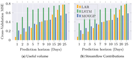
Figure 5.
Cross-validation MSE at a 10-fold time series split for Linear AutoRegressive, LSTM, and MOVGP models along the prediction horizon.
At the testing stage, trained LAR, LSTM, and MOVGP models forecast the last 365 days on the dataset for both time series at each horizon considered. Figure 6 depicts reservoir-wise testing MSE boxplots computed over the 10 prediction horizons for the Streamflow Contributions. Note that reservoir T makes the models perform the worst, whereas reservoir D becomes the least challenging. Moreover, the widespread error at reservoir L contrasts with the small dispersion at reservoir D. Therefore, varying boxplots advise the changing forecasting complexity over the horizons and reservoirs despite corresponding to the same hydrological time series. According to the grand averages in dashed lines, the MOVGP model obtains the best average performance, followed by the LAR. Thus, for the Contributions time series, MOGP offers a better explanation for nonlinearities in the data than LSTM.
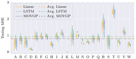
Figure 6.
Distribution for the testing MSE of contrasted approaches at each reservoir for the Streamflow Contributions. Statistics are computed over the 10 prediction horizons. The dashed line averages the reservoir-wise MSE.
Figure 7 offers time series plots for Useful Volume and Contributions with their respective one-day horizon predictions from the forecast models for three reservoirs of interest. Notice, in Figure 7a, that the MOVGP and Linear models reach a well-fit prediction and learn the smoothness of the reservoir data, but the MOVGP model presents the advantage of yielding a predictive distribution and, therefore, a confidence interval. In addition, the LSTM model shows abrupt changes that deviate from the actual behavior of the curve, producing a higher error. For Figure 7c, a narrow confidence interval describes the time series noise. Observe the presence of a peak at day 65 that is out of the confidence interval, possibly an outlier classified as an anomaly by predictive distribution offered by the MOVGP model.
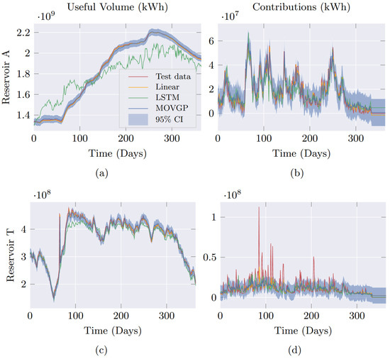
Figure 7.
Useful volume (left) and contributions (right) forecasted by the contrasting approaches on one-year test data at reservoirs A, K, and T (top to bottom) and one-day prediction horizon .
In the case of the Streamflow Contributions, the three models closely follow the abrupt curve trend and lie within the confidence intervals for reservoir A in Figure 7b. Lastly, Figure 7d displays peaks in the Streamflow Contributions of reservoir T. Although no model catches the peak’s tendency, MOVGP explains them as outliers because of the predictive distribution. In this way, the MOVGP model is less influenced by anomalies, producing better generalization and, thus, outperforming the other models.
4. Concluding Remarks
This work proposed a forecasting methodology for multiple output prediction of Useful Volume and Streamflow Contributions of Colombian reservoirs using Variational Gaussian Processes. Since the coregionalization of MOVGPs imposes a unique latent process, generating multiple outputs, we devoted a single model for each hydrological variable to minimize overgeneralization issues. The proposed MOVGP was compared against LSTM-based and Linear AutoRegressive models using actual time series. The hyperparameter tuning stage proved that MOVGP suitably adapted to time complexity by optimizing the number of latent variables and inducing points to control model flexibility. The comparison in testing data, shown in Figure 5, revealed that the MOVGP outperformed the others in predicting long-term horizons, particularly when the linear model missed relationships between inputs and outputs. Therefore, MOVGP outperforms hydrological forecasting, providing prediction reliability and outlier detection through the predictive distribution.
For future work, we devise the following research directions. First, we will extend the methodology to support energy-related time series such as daily thermoelectric schedules. Secondly, we will develop deep learning models to learn complex patterns in hydrological time series.
Finally, to overcome the overgeneralization and linear coregionalization restriction issues, we will work on time-variant convolutional kernel integration.
Author Contributions
Conceptualization, J.D.P.-C.; Data Extraction, Á.A.O.-G. and M.H.-L.; Validation, D.A.C.-P. and G.C.-D.; Original Draft Preparation, J.D.P.-C., Á.A.O.-G. and D.A.C.-P.; Review and Editing, J.D.P.-C. and D.A.C.-P. All authors have read and agreed to the published version of the manuscript.
Funding
This research was funded by the Minciencias project: “Desarrollo de una herramienta para la planeación a largo plazo de la operación del sistema de transporte de gas natural de Colombia”—código de registro 69982—CONVOCATORIA DE PROYECTOS CONECTANDO CONOCIMIENTO 2019 852-2019.
Institutional Review Board Statement
Not applicable.
Informed Consent Statement
Not applicable.
Data Availability Statement
Not applicable.
Acknowledgments
Thanks to the Maestría en Ingeniería Eléctrica, graduate program of the Universidad Tecnológica de Pereira.
Conflicts of Interest
The authors declare no conflict of interest.
References
- Basu, M. Improved differential evolution for short-term hydrothermal scheduling. Int. J. Electr. Power Energy Syst. 2014, 58, 91–100. [Google Scholar] [CrossRef]
- Nazari-Heris, M.; Mohammadi-Ivatloo, B.; Gharehpetian, G.B. Short-term scheduling of hydro-based power plants considering application of heuristic algorithms: A comprehensive review. Renew. Sustain. Energy Rev. 2017, 74, 116–129. [Google Scholar] [CrossRef]
- Freire, P.K.D.M.M.; Santos, C.A.G.; Silva, G.B.L.D. Analysis of the use of discrete wavelet transforms coupled with ANN for short-term streamflow forecasting. Appl. Soft Comput. J. 2019, 80, 494–505. [Google Scholar] [CrossRef]
- XM. La Generación de Energía en enero fue de 6276.74 gwh. 2022. Available online: https://www.xm.com.co/noticias/4630-la-generacion-de-energia-en-enero-fue-de-627674-gwh (accessed on 7 November 2022).
- Cheng, M.; Fang, F.; Kinouchi, T.; Navon, I.; Pain, C. Long lead-time daily and monthly streamflow forecasting using machine learning methods. J. Hydrol. 2020, 590, 125376. [Google Scholar] [CrossRef]
- Yaseen, Z.M.; Allawi, M.F.; Yousif, A.A.; Jaafar, O.; Hamzah, F.M.; El-Shafie, A. Non-tuned machine learning approach for hydrological time series forecasting. Neural Comput. Appl. 2018, 30, 1479–1491. [Google Scholar] [CrossRef]
- Mosavi, A.; Ozturk, P.; Chau, K.W. Flood prediction using machine learning models: Literature review. Water 2018, 10, 1536. [Google Scholar] [CrossRef]
- Apaydin, H.; Feizi, H.; Sattari, M.T.; Colak, M.S.; Shamshirband, S.; Chau, K. Comparative analysis of recurrent neural network architectures for reservoir inflow forecasting. Water 2020, 12, 1500. [Google Scholar] [CrossRef]
- Zhu, S.; Luo, X.; Xu, Z.; Ye, L. Seasonal streamflow forecasts using mixture-kernel GPR and advanced methods of input variable selection. Hydrol. Res. 2019, 50, 200–214. [Google Scholar] [CrossRef]
- Saraiva, S.V.; de Oliveira Carvalho, F.; Santos, C.A.G.; Barreto, L.C.; de Macedo Machado Freire, P.K. Daily streamflow forecasting in Sobradinho Reservoir using machine learning models coupled with wavelet transform and bootstrapping. Appl. Soft Comput. 2021, 102, 107081. [Google Scholar] [CrossRef]
- Ni, L.; Wang, D.; Wu, J.; Wang, Y.; Tao, Y.; Zhang, J.; Liu, J. Streamflow forecasting using extreme gradient boosting model coupled with Gaussian mixture model. J. Hydrol. 2020, 586, 124901. [Google Scholar] [CrossRef]
- Sun, A.Y.; Wang, D.; Xu, X. Monthly streamflow forecasting using Gaussian process regression. J. Hydrol. 2014, 511, 72–81. [Google Scholar] [CrossRef]
- Niu, W.; Feng, Z. Evaluating the performances of several artificial intelligence methods in forecasting daily streamflow time series for sustainable water resources management. Sustain. Cities Soc. 2021, 64, 102562. [Google Scholar] [CrossRef]
- Zhu, S.; Luo, X.; Yuan, X.; Xu, Z. An improved long short-term memory network for streamflow forecasting in the upper Yangtze River. Stoch. Environ. Res. Risk Assess. 2020, 34, 1313–1329. [Google Scholar] [CrossRef]
- Moreno-Muñoz, P.; Artés, A.; Álvarez, M. Heterogeneous Multi-output Gaussian Process Prediction. In Proceedings of the Advances in Neural Information Processing Systems; Bengio, S., Wallach, H., Larochelle, H., Grauman, K., Cesa-Bianchi, N., Garnett, R., Eds.; Curran Associates, Inc.: New York, NY, USA, 2018; Volume 31. [Google Scholar]
- Rasmussen, C.E.; Williams, C.K.I. Gaussian Processes for Machine Learning; Adaptive Computation and Machine Learning; MIT Press: Cambridge, MA, USA, 2006; pp. 1–248. [Google Scholar]
- Liu, H.; Cai, J.; Ong, Y.S. Remarks on multi-output Gaussian process regression. Knowl.-Based Syst. 2018, 144, 102–121. [Google Scholar] [CrossRef]
- Álvarez, M.A.; Rosasco, L.; Lawrence, N.D. Kernels for Vector-Valued Functions: A Review. Found. Trends® Mach. Learn. 2012, 4, 195–266. [Google Scholar] [CrossRef]
- Hensman, J.; Fusi, N.; Lawrence, N.D. Gaussian Processes for Big Data. arXiv 2013, arXiv:1309.6835. [Google Scholar] [CrossRef]
- Hensman, J.; Matthews, A.; Ghahramani, Z. Scalable Variational Gaussian Process Classification. arXiv 2014, arXiv:1411.2005. [Google Scholar] [CrossRef]


Disclaimer/Publisher’s Note: The statements, opinions and data contained in all publications are solely those of the individual author(s) and contributor(s) and not of MDPI and/or the editor(s). MDPI and/or the editor(s) disclaim responsibility for any injury to people or property resulting from any ideas, methods, instructions or products referred to in the content. |
© 2023 by the authors. Licensee MDPI, Basel, Switzerland. This article is an open access article distributed under the terms and conditions of the Creative Commons Attribution (CC BY) license (https://creativecommons.org/licenses/by/4.0/).