Abstract
This study compares three methods for optimizing the hyper-parameters m (embedding dimension) and (time delay) from Taken’s Theorem for time-series forecasting to train a Support Vector Regression system (SVR). Firstly, we use a method which utilizes Mutual Information for optimizing and a technique referred to as “Dimension Congruence” to optimize m. Secondly, we employ a grid search and random search, combined with a cross-validation scheme, to optimize m and hyper-parameters. Lastly, various real-world time series are used to analyze the three proposed strategies.
1. Introduction
Several complex phenomena are often modeled as a sequence of states. This sequence is known as the phase space. A time series is a finite sequence of states in a dynamical system measured directly or indirectly. A relevant approach to perform time series analysis is Taken’s embedding theorem [1], which states that, from a sequence of states (i.e., time series) in a dynamical system, it is possible to generate all the system’s phase space U. More specifically, for a sequence of observations x of dimension m (embedding dimension) and a constant (time delay), there exists a function f such as:
From Equation (1) it can be inferred that, given a time series S, it is possible to predict the state at time t (hereafter, ) by using m previous observations sampled at frequency . The two problems, and their solutions, are the following: the function f is often too complex to be found analytically, which is when machine learning algorithms comes into play with the objective of using a supervised learning algorithm to learn f; it is necessary to find the correct modeling for the time series, i.e., the optimal values for m and , for which Random search, Grid search, and Mutual information + Dimension Congruence can be used.
2. Theoretical Background
Given Equation (1), the first task is to find the optimal value for the time delay and embedding dimension m.
2.1. Mutual Information
Regarding the , in [2] Cao, L. proposes using mutual information. The process relies on making and as independent as possible to maximize the information obtained from each variable in the reconstruction of the phase space. To achieve this, the mutual information function (2) can be applied:
Note the similarity of this with entropy, i.e., this function measures how surprising it is that results, given that resulted, i.e., when and are very independent, then . To find the it is, therefore, enough to minimize the function (2).
Once the is fixed, it is necessary to find the embedding dimension m. The latter is achieved by using the false neighbors [2] to determine the dimension congruence.
2.2. Dimension Congruence
The aim of this procedure is for the distances between neighbors (data close to each another) on dimension m of Equation (1) to be constant. To this end, firstly, the distance between and in the dimension m is defined as the maximum between the differences of their components, as in Equation (3):
Now, we can say that the nearest neighbor of is if is satisfied such that:
where n is the sample size, it is worth mentioning that depends on t so we call it and then we define the “nearest neighbor” congruence of in m as:
Note that in if is sufficiently congruent being the nearest neighbor of in m, there is the possibility to define the “dimension congruence” of m as follows:
In summary, the dimension congruence measures how true it is that the nearest neighbors continue to be nearest neighbors as the dimension increases, which is useful, given the assumption that there is an attractor in the system under study [2].
In this work, m was selected as lower m satisfying . As alternative strategies to find m and , Evolutionary computation algorithms, Random Search(RS) and Grid Search (GS) can be used. In this paper we focus on comparing Mutual Information + Dimension Congruence with RS and GS, given [3], which states that random search is good enough for parameter optimization.
2.3. Random Search
Let f be a model that depends on a parameter . The random search method [3] involves defining a range for , a probability distribution , and the number of values to be tested. Then, n parameters are drawn from the distribution g, and the behavior of each of the corresponding models is evaluated by computing a fitness function. The best-performing model, , is selected based on the fitness value.
2.4. Grid Search
In contrast with random search, the grid search method [4] involves sampling values equally spaced in the range , specifically, .
From Figure 1 we can appreciate the differences between random search and grid search.
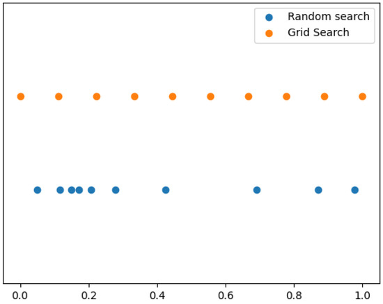
Figure 1.
Differences between Random Search and Grid Search.
Having described the procedures for finding m and , it is time to describe the fitness measures used.
2.5. Fitness Function
The Mean Absolute Percentage Error (MAPE) is the fitness function determining the optimal value for parameters m and . Additionally, the Mean Squared Error (MSE) and the Coefficient of Determination () were used to compare the three optimization procedures with MAPE. For completeness, a brief description of each one is provided.
2.5.1. MAPE
MAPE [5] is a widely used measure in time series forecasting and seems to yield good results. Note that in Equation (7) MAPE takes the average of the absolute value of the errors expressed as a percentage of the actual value, and if it approaches 0 the better the fit, while if it approaches ∞ the worse the fit.
2.5.2. MSE
Ref. [6] is the average of the squared errors. If the model fits perfectly then . The closer it is to ∞ the worse it is. It is computed by using Equation (8):
2.5.3.
Ref. [7] calculates the ratio between the model’s variance and the actual data’s variance. In other words, it ascertains how similar the predicted and actual data variances are. If they are equal, is equal to 1, which means the model fits perfectly. The worse value for is . To find Equation (9) is used:
Finally, in the next section we describe the models we used for the experiments.
2.6. Support Vector Regression Algorithm (SVR)
The SVR algorithm is based on Support Vector Machine (SVM) Algorithm [8]. SVM is an algorithm for separating samples depending on the class they belong to. The algorithm works by increasing the size of the sample space via a kernel, and in that larger size, three parallel hyperplanes are constructed, separated by an distance each. The main idea is to optimize the kernel and the hyperplanes so that only a small number of samples, controlled by the parameter , are outside the region to which they belong, i.e., the samples of one class belong to one side of the hypertube and those of the other class belong to the other side of the hypertube.
On the other hand, SVR aims for all the samples to be inside the hypertube and only a small amount of samples to be outside the hypertube, controlled by the parameter , and, thus, uses the image of the central hyperplane projected in the original space to predict future values of the time series.
- , and are the parallel hyperplanes.
- is located at a distance above .
- is located at a distance below .
- Then and form the hypertube
- The quantity is the minimum possible, subject to
Where is the SVR kernel weight and is the distance that the i-th data moves away from the hypertube, while C is a regularization parameter.
Note how the larger c is, the less freedom the data have to move out of the hypertube. The idea is to find a hypertube that approximates the data.
3. Experiments and Results
The study focused on six real-world time series, each representing a measurement of a real-world phenomenon. The aim was to examine more complex time series than artificially generated ones. The selected time series displayed a wide range of characteristics, including exponential and moderate growth patterns, general trends, and horizontal patterns. The goal was to evaluate the generalization ability of the proposed methodologies by considering time series with diverse characteristics. Below is a brief description of each of the time series used.
3.1. SARS-CoV-2 in Mexico (COV)
The time series data for this study was obtained from the General Direction of Epidemiology (https://www.gob.mx/salud/documentos/datos-abiertos-152127 (accessed on 19 December 2022)). It consists of the confirmed and suspected COVID-19 cases in Mexico. The data spans 1025 days, and the number of confirmed cases per laboratory ranges from 0 to 9800. The data were normalized such that the number of cases fell from 0 to 1. For the purposes of this study, this time series is referred to as COV. Figure 2a depicts the evolution of the COV time series.
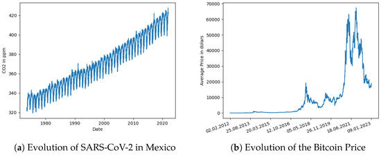
Figure 2.
Covid and Bitcoin.
3.1.1. Bitcoin Price on Bitfinex (BIT)
This time series comprises daily variations in the price of Bitcoin in dollars, recorded on the Bitfinex platform between February 2012 and January 2023 (The data is available at https://www.investing.com/crypto/bitcoin/btc-usd-historical-data (accessed on 10 February 2023)). The dataset includes the daily high and low prices. The average price is computed as . The time series were normalized between 0 and 1 for consistent analysis with the other time series used in this study. Figure 2b displays the evolution of the BIT time series.
3.1.2. Air Temperature in Acuitzio del Canje (TEM)
This time series consists of temperature data recorded by the MXN00016001 weather station located in Acuitzio del Canje between 2004 and 2007 (The data was obtained from https://www.ncei.noaa.gov/ (accessed on 15 January 2023)). The dataset comprises 1401 data points of daily minimum and maximum temperatures. The average temperature is calculated as . The data is recorded in degrees Fahrenheit and was subsequently normalized between 0 and 1 for comparison with other time series in this study. The evolution of the TEM time series is depicted in Figure 3a.
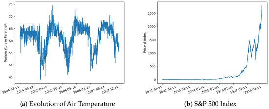
Figure 3.
Temperature and S&P.
3.1.3. S&P500 Index
The S&P500 index series (Data was sourced from: https://datahub.io/core/s-and-p-500 (accessed on 11 February 2023)) is a monthly measurement of the value of the S&P500 stock index, which represents the 500 most valuable companies in the United States. It consists of 1768 monthly value data points calculated from 1871 to 2018. The data was normalized for analysis between the range of . Figure 3b shows the evolution of the S&P500 index graphically.
3.1.4. Seismic Activity in Michoacán
This series comprises seismic activity recorded by the National Seismological System in Michoacán (The time series is available at the following URL: http://www2.ssn.unam.mx:8080/catalogo/ (accessed on 22 January 2023)). The values cover the period from 1988 to 2023. This time series was of interest as the data was not evenly spaced. One possibility was to summarize the data to create an indicator to identify “how active each month was”. However, for our study, the original sampling frequency was maintained. Each event is a numerical value representing its magnitude in Richter scale degrees and consists of 17,500 data points, which were normalized between . Figure 4a graphically depicts these data.
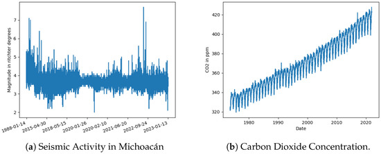
Figure 4.
Seismicity and .
3.1.5. Atmospheric Carbon Dioxide Concentration
This is a series of daily atmospheric carbon dioxide (CO) concentration measurements taken at the Barrow Atmospheric Baseline Observatory (Data obtained from https://www.co2.earth/daily-co2 (accessed on 9 February 2023)) in the United States. The CO concentrations are reported in parts per million (ppm) and cover the period from 1973 to 2021. To facilitate the analysis and interpretation of the data, all the values were normalized to the range of .
Figure 4b shows this time series.
3.2. Experimental Setup
For each of the analyzed time series, the parameters m,, and the parameters C and for the SVR were optimized. Three strategies were used: mutual information + congruence, grid search, and random search. The flow diagram in Figure 5 summarizes the process.
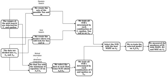
Figure 5.
Flow diagram of each procedure applied to each time series.
The diagram in Figure 5 illustrates the general overview of the three procedures applied to each time series. It is noteworthy that the final outcome for each time series were nine goodness of fit measures. These measures were then used to compare the procedures. Before diving into the specifics of each process, it is essential to consider a few key points.
The data were divided into three sets:
- Set contained the last of the data to be used for testing and calculating the model’s fitness.
- Set contained the last of the data once set had been removed, to be used for hyper-parameter tuning.
- Set consisted of the remaining data to be used for training the parameters.
All of the models used were Support Vector Regression (SVR), and for the SVR C and hyper-parameters, the following applied:
- Grid search was used to find the C and for all SVR models.
- The grid for C values was in .
- The grid for values was .
For RS and GS of and m, the following conditions were met:
- The sets , contained all possible values of and m for each time series, and each procedure (Random Search and Grid Search) had 20 elements (for computational capacity reasons).
- The infimum of these sets was always 2.
- The supremum was always (so that ).
- The distribution used for the random search was always uniform.
With this in mind, the procedures used to search m (dimension of the reconstructed phase space) and (delay) were:
- Mutual information + dimension congruence:
- 1.
- Find using the mutual information function from Equation (2) on , and take the minimum.
- 2.
- Find the embedding dimension by selecting the first m that satisfies in Equation (6) with the obtained on .
- 3.
- Train all possible SVRs determined by the elements of on .
- 4.
- Select the model having MAPE on which is the minimum.
- 5.
- Measure the goodness of the selected model using MAPE on .
- Random search and grid search:
- 1.
- Use each element of to train models on .
- 2.
- Select the model having MAPE on which is the minimum.
- 3.
- Measure the goodness of the selected model using MAPE on .
It is worth mentioning that the parameter space in both the grid search and the random search was not very large due to the lack of hardware. It is to be expected that enlarging the size of these spaces would improve the results.
Upon completion of the procedures, a comparison was made by evaluating the distributions generated by each of the fitness measures obtained by each proposed method.
3.3. Results
Table 1 shows the results for the three metrics. The MAPE, evaluation, and MSE, best results are boldfaced. For instance, in the series “BIT” GS was the best procedure with respect to MAPE, but also with respect to and with respect to MSE. As you can see, there was no procedure that was always better than another. There were some series where RS and IC were better than RS. However, it is essential to clarify that even though GS had better results, it is a brute force algorithm, in that, although it has better optimizations, the computational cost is too high (RS and GS take in the order of hours, while IC takes in the order of minutes, on a i9 7th generation). From the results, it is recommended to work with IC to optimize the and m parameters, and, for the regression system parameters, to use RS. It is relevant to point out that IC is the fastest, while it provides a competitive prediction performance.

Table 1.
Quality measurements for each time series made with each one of the proposed optimization strategies.
Figure 6a–c suggests that GS had better results, both in its mean and dispersion. However, if we look only at IC and RS we observe that when one of the two had a better mean, it would also have worse dispersion, which indicates that some series work very well with IC and others with RS, but, in general, it is a good idea to try both methods.

Figure 6.
Boxplots comparing each procedure with different goodness-of-fit measures.
3.4. Future Work
It remains for future work to evaluate the procedures with additional quality measurements. Selecting the model with Mean Squared Logarithmic Error (MSLE) could improve the predictions. Including the regression system in the optimization could improve the prediction performance, by, for instance, using Naïve Bayes and K-Nearest Neighbor systems.
Author Contributions
R.H.-M.: Conceptualization, formal analysis, investigation writing original draft preparation; J.O.-B. (Jose Ortiz-Bejar): Conceptualization, supervision, writing and proofreading; J.O.-B. (Jesus Ortiz-Bejar): Review, formal analysis and proofreading. All authors have read and agreed to the published version of the manuscript.
Funding
This research received no external funding.
Institutional Review Board Statement
Not applicable.
Informed Consent Statement
Not applicable.
Data Availability Statement
Publicly available datasets were analyzed in this study. This data can be found at the URLs mentioned in Section 3 of the manuscript.
Conflicts of Interest
The authors declare no conflict of interest. The authors declare that they have no known competing financial interests or personal relationships that could have appeared to influence the work reported in this paper.
References
- Takens, F. Detecting strange attractors in turbulence. In Dynamical Systems and Turbulence, Warwick; Springer: Berlin/Heidelberg, Germany, 1980; pp. 366–381. [Google Scholar]
- Cao, L. Practical method for determining the minimum embedding dimension of a scalar time series. Phys. D Nonlinear Phenom. 1997, 110, 43–50. [Google Scholar] [CrossRef]
- Bergstra, J.; Bengio, Y. Random Search for Hyper-Parameter Optimization; Universite de Montreal: Montreal, QC, Canada, 2012; Available online: https://www.jmlr.org/papers/volume13/bergstra12a/bergstra12a.pdf (accessed on 10 May 2023).
- Yu, S.; Pritchard, M.; Ma, P.L.; Singh, B.; Silva, S. Two-step hyperparameter optimization method: Accelerating hyperparameter search by using a fraction of a training dataset. arXiv 2023, arXiv:2302.03845. [Google Scholar]
- De Myttenaere, A.; Golden, B.; Le Gr, B.; Rossi, F. Mean Absolute Percentage Error for regression models. Neurocomputing 2016, 192, 38–48. [Google Scholar] [CrossRef]
- Lehmann, E.L.; Casella, G. Theory of Point Estimation, 2nd ed.; Springer: New York, NY, USA, 1998; ISBN 978-0-387-98502-2. [Google Scholar]
- Yin, P.; Fan, X. Estimating R2 Shrinkage in Multiple Regression: A Comparison of Different Analytical Methods. J. Exp. Educ. 2001, 69, 203–224. [Google Scholar] [CrossRef]
- Rivas-Perea, P.; Cota-Ruiz, J.; Chaparro, D.G.; Venzor, J.A.P.; Carreón, A.Q.; Rosiles, J.G. Support Vector Machines for Regression: A Succinct Review of Large-Scale and Linear Programming Formulations. Int. J. Intell. Sci. 2013, 3, 5–14. [Google Scholar] [CrossRef]
Disclaimer/Publisher’s Note: The statements, opinions and data contained in all publications are solely those of the individual author(s) and contributor(s) and not of MDPI and/or the editor(s). MDPI and/or the editor(s) disclaim responsibility for any injury to people or property resulting from any ideas, methods, instructions or products referred to in the content. |
© 2023 by the authors. Licensee MDPI, Basel, Switzerland. This article is an open access article distributed under the terms and conditions of the Creative Commons Attribution (CC BY) license (https://creativecommons.org/licenses/by/4.0/).