Abstract
Triangular fuzzy numbers (TFNs) are used to express the weights of criteria and alternatives to account for the ambiguity and uncertainty inherent to subjective evaluations. However, the proposed method can easily be extended to other fuzzy settings depending on the uncertainty facing managers and decision-makers. Triangular fuzzy number (TFN) is a critical component in building fuzzy models such as fuzzy regression and fuzzy autoregressive. Many symmetrical triangular fuzzy numbers have been proposed to improve the scale’s linguistic accuracy. Additionally, Sturges’ rule is a well-known approach to determining criteria or intervals of grouped data. However, some existing TFN methods are challenging despite being considered in building fuzzy regression models. The increase in electricity distribution is caused by the number of customers and the amount of installed capacity factors in Indonesia. The identified factors are uncertainty, inexactness, and random nature. This paper investigates the residential electricity distribution model using fuzzy regression time series. In the beginning step, the integration between conventional TFN and Sturges’ rule was proposed to determine the criteria or scale of linguistic terms. The secondary data was collected from BPS Indonesia from 2000 to 2021. The dependent variable was denoted as electric power distribution . On the other hand, the number of customers and the amount of installed capacity were grouped as independent variables ( and ). The results showed that the best forecasting model is an FLR right upper limit without constant. This proposed model also has higher MAPE accuracy at 1.44% compared to classical models. Additionally, the proposed triangular fuzzy number could improve the accuracy of the proposed model significantly. Interestingly, both dependent and independent factors were initially forecasted using a basic time series model, namely exponential smoothing.
1. Introduction
The conventional ordinary regression method requires very strict statistical assumptions such as linearity of variables, no multicollinearity among independent variables, homoskedasticity, reliability of measurement, error should be normally distributed and independently [1]. All assumptions above should be provided completely to attain the best regression model. Additionally, the input information related to data quality is a highly indispensable component that should be considered for this method. However, this regression method will not be effective and is not recommended for limited data size and linguistic variables. Based on a systematic review paper, multiple linear regression, general linear regression, polynomial regression, exponential regression, and multivariate adaptive regression spline are frequently implemented for electricity load consumption forecasting models [2].
In previous studies, some non-statistical methods, such as fuzzy regression, fuzzy autoregressive, general regression neural network, kernel regression with -nearest neighbors, and fuzzy time series, have been integrated with ordinary regression to handle the previously-mentioned limitations [3,4,5,6]. Its applications are commonly employed for electricity forecasting [2]. For example, one of them is the integration between fuzzy and regression methods in handling some issues like linguistic data, small-size data, and normality data. Fuzzy regression estimates parameters using the fuzzy optimization approach more effectively than the ordinary least square [7,8]. Some fuzzy regression methods consider the triangular fuzzy number (TFN) for data pre-processing [9].
In each country, electricity forecasting and its models are the main components to be managed and projected by state and private companies for efficient operations of power distribution systems in supporting daily life activities [10,11]. The conventional models have been discussed and implemented by previous researchers to investigate electricity power distribution and its factors using conventional regression or time series. However, the highest forecasting accuracy is an arduous task since various unpredictable factors may influence electricity power distributions.
Hybrid models have been introduced to improve elements, such as forecasting accuracy and data size. Fuzzy regression is one of the hybrid model types in electricity forecasting [12,13,14]. This model deals with the triangular fuzzy number (TFN) of fuzzy form data and is not strictly vital in terms of statistical assumptions [15,16,17]. In this paper, time series analysis is proposed to support fuzzy regression in predicting the value of each variable (dependent and independent) by following a series of times (yearly data). Because the fuzzy regression model is suitable for estimating the significant relationship between dependent and independent variables using fuzzy parameters, it is not a recommended model to forecast future values of variables, especially time series data. Thus, an exponential smoothing model is more practical for such forecasting purposes. Essentially, there are two forecasting phases in this paper.
2. Fundamental Concept
2.1. Triangular Fuzzy Number (TFN)
In 1965, the concepts of fuzzy set and membership function were first proposed by Zadeh [18,19,20]. Some basic notions on fuzzy sets and numbers are included below:
Definition 1.
Fuzzy sets
A fuzzy set of a universal set is defined as follows:
where is the membership function of the set A. The membership value indicates the degree of membership of to the set .
Definition 2.
Triangular Fuzzy Number (TFN)
Let a, b and c be real numbers with, . Then, the triangular fuzzy number (TFN), = (a, b, c) is the fuzzy number (FN) with a membership function [18].
Thus, Equation (1) is interpreted as membership functions as shown in Figure 1.
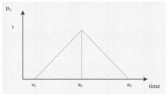
Figure 1.
Triangular fuzzy number = (, ).
Based on Equation (1), a TFN can be defined as:
Based on Equation (2), if the TFN is symmetrical, then is denoted as
where is a spread of TFN and is a non-fuzzy number if .
2.2. Fuzzy Regression Model (FRM)
Fuzzy least square and fuzzy linear regression models have been introduced by Tanaka in 1982. Both models used fuzzy forms in terms of input, process, and output, respectively. Mathematically, FRM with and without intercept is written as [21]:
and
From Equations (4) and (5), , while is a mid-value of j and reveals a spread value of j. Both equations are detailed in Table 1.

Table 1.
General FRM based on intercept and bound functions.
Based on Table 1, some extension models have been proposed by previous researchers [21,22,23] to handle the limitation and minimize the spread of the triangular fuzzy number (TFN) from FRM, as presented in Table 2.
Table 2.
Extended FRM based on [11,12,13].
From Table 2, the general FRM has been extended in terms of objective and constraint functions, respectively. All extended models will be used to estimate the significant factors that contribute to the electricity power distribution for residential sectors in Indonesia from 2000–2016.
2.3. Exponential Smoothing Model (ESM)
In time series data analysis, ESM is widely used for estimating in the light of more recent in an exponentially decreasing manner. The most recent observation receives the most weight, (where ); the second most recent observation receives less weight, ; the observation of two time periods in the past receives even less weight, ; and so forth. Formally, ESM is written mathematically as below [24,25]:
From Equation (6), is a new smoothed value or the forecast value for the next period, is the smoothing constant, is a new observation or the actual value of the series in period , and is the old-smoothed value or the forecast for period . This model is also frequently applied to the forecast of electricity load demand data.
3. Forecasting Model for Electricity Power Distribution
In this paper, we considered three phases on electricity power distribution and its factors were proposed based on three different forecasting models as illustrated in Figure 2.
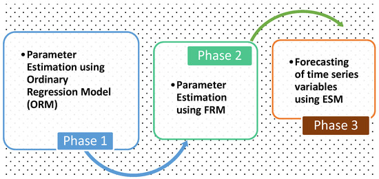
Figure 2.
Phase on building an electricity forecasting model.
Based on Figure 2, FRM can be applied if the ORM has been established in the first phase. All slopes or parameters obtained from the ORM will be used to formulate a fuzzy linear programming model. From the FRM, some possibilistic models will be obtained, as described in Table 2, respectively. Measurement error using mean absolute percentage error (MAPE) through data training-testing will be considered to choose the best FR. At the end of the process, ESM will be implemented to forecast the electricity power distribution and its factors for the residential sector by following a series of times (yearly data).
4. Empirical Study
In this section, the implementation of the suggested phases is attempted in two case studies as follows:
Case study A: Electricity power distribution
Step 1: Build ORM for electricity power distribution using secondary data [26] as presented in Table 3.
Table 3.
ORM for electricity power distribution data.
Step 2: Transform single data into symmetrical TFN forms for electricity power distribution and its factors using Sturges rule as follows:
- Determine range (R) data for each dependent and independent variable.
- Determine .
- Determine .
- Determine lower and upper limits of intervals.
- Provide a distribution table.
For example, the transformation value of customer numbers is illustrated in Figure 3.
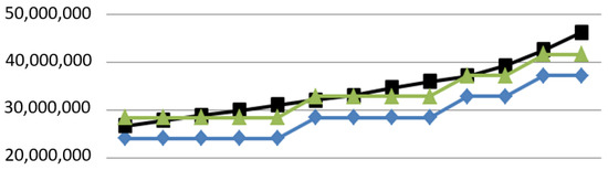
Figure 3.
Number of customers in TFN form using Sturges.
Step 3: The estimates of fuzzy parameters presented in Table 4 illustrate the building of fuzzy optimization.
Table 4.
Fuzzy parameters estimation.
Table 4 shows the minimization of the spread function () from the mid value () using fuzzy intervals to left-right constraints.
Step 4: Based on parameters obtained in Step 3, build FRMs as presented in Table 5.
Table 5.
FRM for left and right sides.
Table 5 shows that the left and right sides have three different FRMs, respectively. Furthermore, these models will be used for forecasting purposes using training and testing data in Step 5.
Step 5: Forecast electricity power distribution using all possible FRM as expressed in Table 6, respectively.
Table 6.
Forecast values using left-right sides FRM.
Step 6: Evaluate and validate all possible FRMs using MAPE of training and testing data, respectively, as presented in Table 7.
Table 7.
MAPE training-testing of FRM.
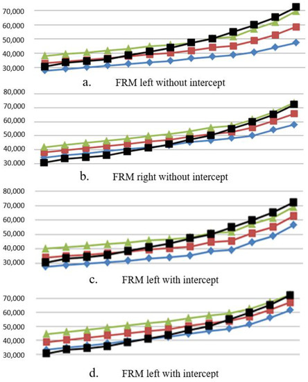
Figure 4.
Actual and forecasted values using various FRM.
Step 7: Forecast electricity power distribution for 2016–2021 using the best FRM model (smallest MAPE) without intercept and exponential smoothing (ES) as presented in Table 8 and Table 9, respectively.
Table 8.
Testing data for 2016.
Table 9.
Testing data for 2017–2021.
Based on Table 8, electricity power distribution () is predicted using FRM right without intercept, as expressed in Table 7. On a regular basis, a regression model is not directly practical for forecasting purposes. In this case, each variable was gathered and measured by considering time intervals (yearly time series data). Thus, they should be predicted separately using time series models such as exponential smoothing (ES). Additionally, each forecasted value was obtained from the ES model, respectively.
In the final stage, the prediction of power distribution can be substituted into FRM right model as written in Equation (7):
From this table, the predicted values were obtained using Equation (7) and ES model. Actual power distribution was 93,634.63 GWh in 2016. On a note, the predicted and actual values revealed immense differences because the State Electricity Company of Indonesia offered a power subsidy for the residential sector for that year. Additionally, the national championship sports of Indonesia were also conducted in 2016. Therefore, the electricity distribution exceeded the actual amount. In this case, two forecasting parts, namely parameter estimation using fuzzy regression and future amount estimation, were already taken into account using the exponential smoothing technique. Unlike some previous studies [11,12,13,14], the researchers were only concerned with the fuzzy regression part.
The State Electricity Company of Indonesia offers subsidies for their customers every year. Thus, the proposed model lacks the ability to capture the actual amount. Occasionally, the difference is also significant between forecasted and actual amounts.
Case study B: Palm oil production
By following the same steps given in Case study A, the comparison between actual and forecast values can be shown for palm oil data from January–December 2012 in Table 10, Table 11 and Table 12, respectively.
Table 10.
Forecast values of monthly palm oil production using left-right sides FRM.
Table 11.
MAPE training-testing data with and without intercept using FRM.
Table 12.
Testing data for January 2013.
5. Conclusions
In this paper, the parameters (intercept and slopes) of ordinary regression in building fuzzy linear regression were implemented. Both parameters were employed for fuzzy optimization purposes, namely objective function and left-right constraints. Furthermore, the Sturges rule was used to determine the symmetrical TFN and the number of fuzzy intervals when the total number of observations was specified.
In application, FRM without intercept was considered to capture the actual electricity data precisely. Each variable from FRM was predicted using a basic time series technique known as exponential smoothing. Therefore, two types of forecasting strategies have been employed to estimate yearly electricity power distribution in Indonesia from 2000 to 2021 and palm oil production. In this paper, we also considered the effectiveness between with and without intercepts in the forecasting models.
Author Contributions
Conceptualization, R.E., S.R.W. and E.E.; methodology, N.W.M.Y.; software, E.H.P. and R.S.; data analysis, R.E., A.H. and M.S.; data interpretation, A.H. and M.S.; writing—preparation, R.E. and S.R.W.; writing—editing, S.R.W. and R.S.; visualization, E.H.P. All authors have read and agreed to the published version of the manuscript.
Funding
This research received no external funding.
Institutional Review Board Statement
Not applicable.
Informed Consent Statement
Not applicable.
Data Availability Statement
No new data are created and analyzed in this paper. Data sharing is not allowed.
Acknowledgments
The authors acknowledge all possible administrative and financial support provided by our institute, i.e., “Academic Affair and International Relation, Universiti Pendidikan Sultan Idris, Malaysia” to conduct and publish this research work.
Conflicts of Interest
The authors declare no conflict of interest.
References
- Franzco, R.J.C.D.P.; Farmer, L.D.M. Review understanding and checking the assumptions of linear regression: A primer for medical researchers. Clin. Exp. Ophthalmol. 2014, 42, 590–596. [Google Scholar]
- Zhang, L.; Wen, J.; Li, Y.; Chen, J.; Ye, Y.; Fu, Y.; Livingood, W. A Review of Machine Learning in Building Load Prediction. Appl. Energy 2021, 285, 116452. [Google Scholar] [CrossRef]
- Ismail, Z.; Efendi, R.; Deris, M.M. Interquartile Range Approach to Length-Interval Adjustment of Enrolment Data in Fuzzy Time Series Forecasting. Int. J. Comp. Intell. Appl. 2012, 12, 1350016. [Google Scholar] [CrossRef]
- Efendi, R.; Arbaiy, N.; Deris, M.M. A New Procedure in Stock Market Forecasting Based on Fuzzy Random Auto-Regression Time Series Model. Inf. Sci. 2018, 441, 113–132. [Google Scholar] [CrossRef]
- Efendi, R.; Deris, M.M. Non-probabilistic inverse fuzzy model in time series forecasting. Int. J. Uncertain. Fuzziness Knowl.-Based Syst. 2018, 26, 855–873. [Google Scholar] [CrossRef]
- Sturges, H. The Choice of A Class-Interval. J. Am. Stat. Assoc. 1926, 21, 65–66. [Google Scholar] [CrossRef]
- Tanaka, H. Fuzzy Data Analysis by Possibilistic Linear Models. Fuzzy Sets Syst. 1987, 24, 363–375. [Google Scholar] [CrossRef]
- Tanaka, H.; Watada, J. Possibilistic linear systems and their application to the linear regression model. Fuzzy Sets Syst. 1988, 27, 275–289. [Google Scholar] [CrossRef]
- Wang, H.M.; Lee, M.J. Fuzzy regression model with fuzzy input and output data. Inf. Sci. 2007, 177, 2049–2067. [Google Scholar]
- Rosadi, M.; Syamsul, A.B. Faktor-Faktor yang Mempengaruhi Konsumsi Listrik di Indonesia. J. Kaji. Ekon. Dan Pembang. 2019, 1, 273–286. [Google Scholar] [CrossRef]
- Nazarko, J.; Zalewski, W. The fuzzy regression approach to peak load estimation in power distribution systems. IEEE Trans. Power Syst. 1999, 14, 809–814. [Google Scholar] [CrossRef]
- Purwareta, H.P.; Gusti, N.I.; Nuri, W. Model Peramalan Pasokan Energi Primer dengan Pendekatan Metode Fuzzy Linear Regression (FLR). J. Sains Dan Seni ITS 2012, 1, A34–A39. [Google Scholar]
- Khairudin, M.; Nursusanto, U.; Ismara, K.I.; Arifin, F.; Fahrurrozi, D.B.; Yahya, A.; Prabuwono, A.S.; Mohamed, Z. Estimated Use of Electrical Load Using Regression Analysis and Adaptive Neoro Fuzzy Inference System. J. Eng. Sci. Technol. 2021, 16, 4452–4467. [Google Scholar]
- Lee, G.-C. Regression-Based Methods for Daily Peak Load Forecasting in South Korea. Sustainability 2022, 14, 3984. [Google Scholar] [CrossRef]
- Lah, M.S.C.; Arbaiy, N.; Efendi, R. Stock Market Forecasting Model Based on AR(1) with Adjusted Triangular Fuzzy Number Using Standard Deviation Approach for ASEAN Countries. Intell. Interact. Comput. 2019, 67, 103–114. [Google Scholar]
- Efendi, R.; Imandari, A.N.; Rahmadhani, Y.; Suhartono; Samsudin, N.A.; Arbai, N.; Deris, M.M. Fuzzy autoregressive time series model based on symmetry triangular fuzzy numbers. New Math. Nat. Comput. 2021, 17, 387–401. [Google Scholar] [CrossRef]
- Azadeh, A.; Khakestani, M.; Saberi, M.A. Flexible Fuzzy Regression Algorithm for Forecasting Oil Consumption Estimation. J. Energy Policy 2009, 37, 5567–5579. [Google Scholar] [CrossRef]
- Mir, A.A.; Alghassab, M.; Ullah, K.; Khan, Z.A.; Lu, Y.; Imran, M. A Review of Electricity Demand Forecasting in Low and Middle Income Countries: The Demand Determinants and Horizons. Sustainability 2020, 12, 5931. [Google Scholar] [CrossRef]
- Zadeh, L.A. Fuzzy sets. Inf. Control 1965, 8, 338–353. [Google Scholar] [CrossRef]
- Afrasiabi, A.; Tavana, M.; Caprio, D.D. An Extended Hybrid Fuzzy Multi-Criteria Decision Model for Sustainable and Resilient Supplier Selection. Environ. Sci. Pollut. Res. 2022, 29, 37291–37314. [Google Scholar] [CrossRef]
- Tanaka, H.; Uejima, S.; Asia, K. Linear Regression Analysis with Fuzzy Model. IEEE Trans. Syst. Man Cybern. 1982, 12, 903–907. [Google Scholar]
- Tanaka, H.; Hayashi, I.; Watada, J. Possibilistic Linear Regression Analysis For Fuzzy Data. Eur. J. Oper. Res. 1989, 40, 389–396. [Google Scholar] [CrossRef]
- Chang, Y.H.O.; Ayyub, B.M. Fuzzy Regression Methods-A Comparative Assessment. Fuzzy Sets Syst. 2001, 199, 187–203. [Google Scholar] [CrossRef]
- Wooldridge, M. Introductory Econometrics A Modern Approach, 3rd ed.; South-Western: Mason, OH, USA, 2006. [Google Scholar]
- Hanke, J.E.; Wichern, D.W. Business Forecasting, 9th ed.; Pearson/Prentice Hall: Hoboken, NJ, USA, 2009. [Google Scholar]
- BPS. Available online: https://www.bps.go.id/subject/7/energi.html#subjekViewTab3 (accessed on 20 June 2023).


Disclaimer/Publisher’s Note: The statements, opinions and data contained in all publications are solely those of the individual author(s) and contributor(s) and not of MDPI and/or the editor(s). MDPI and/or the editor(s) disclaim responsibility for any injury to people or property resulting from any ideas, methods, instructions or products referred to in the content. |
© 2023 by the authors. Licensee MDPI, Basel, Switzerland. This article is an open access article distributed under the terms and conditions of the Creative Commons Attribution (CC BY) license (https://creativecommons.org/licenses/by/4.0/).