Abstract
Functional data analysis has demonstrated significant success in time series analysis. In recent biomedical research, it has also been used to analyze sequence variations in genome-wide association studies (GWAS). The observations of genetic variants, called single-nucleotide polymorphisms (SNPs), of an individual are distributed over the loci of a DNA sequence. Thus, it can be regarded as a realization of a stochastic process, which is no different from a time series. However, SNPs are usually coded as the number of minor alleles, which are categorical. The usual least-square smoothing in FDA only works well when the data is continuous and normally distributed. The normality assumption will be violated for categorical SNP data. In this work, we propose a two-step method for smoothing categorical SNPs using a novel method and constructing haplotypes having strong associations with the disease using functional generalized linear models. We show its effectiveness through a real-world PennCATH dataset.
1. Introduction
Functional data analysis (FDA) is a common tool for analyzing complex datasets that are collected over a sequence, such as time and location. It is based on the assumption that there is an underlying stochastic process represented by a continuous function , but the data can only be observed at discrete time points or locations. To overcome this challenge, FDA represents the datasets as functions or curves by smoothing the observations. FDA has found extensive application in many fields related to time series analysis. Examples include predicting stock prices, discovering geophysical and meteorological patterns, and forecasting traffic volumes. Recently, there has been increasing interest in using FDA in biomedical research, such as genome-wide association studies (GWAS).
GWAS aim to find associations between single-nucleotide polymorphisms (SNPs) and diseases or traits by case–control studies, providing insights into the genetic risk factors for diseases and offering opportunities for preventive measures and treatments [1]. As a result, GWAS plays a critical role in personal genomics, and thousands of GWAS have been conducted over the past few decades. Fan et al. [2] have highlighted that genetic variant data can be viewed as a collection of random variables forming a stochastic process, and can be treated as functional data. One of the key advantages of FDA in GWAS is its ability to naturally incorporate the correlation, linkage, and linkage disequilibrium (LD) information of the genetic variants into the association tests. FDA can capture the complex dependency structure and higher order LD among the genetic variants, which is often missed by other methods such as the sequence kernel association test (SKAT) [3] and its optimal unified test (SKAT-O) [4]. Another advantage of the functional data representation is its suitability for large-scale genomic data, providing a computationally efficient way to test the association between multiple variants and the phenotype.
In their work, Fan et al. [2] proposed two methods for fitting the discrete SNP values: either using ordinary least-square smoothers, or approximating SNPs with K functional principal components. The effectiveness of FDA in GWAS, as demonstrated by Fan et al., has also been confirmed in the subsequent studies [5,6,7]. Nevertheless, SNPs are typically coded as the number of minor alleles, resulting in categorical data that violates the normality assumption required for the least-square smoothing. The objective of this paper is to propose a more robust approach to represent genetic variants using functional data analysis, which addresses the problem of normality assumption violation in the least-square smoothing method. In addition, we introduce a two-step method that integrates our novel smoothing method with functional generalized linear models to identify haplotypes, i.e., blocks of SNPs, that are strongly associated with the phenotype.
Our proposed approach is described in detail in the following sections. In Section 2, we describe the PennCATH dataset used in our experiments and explain our two-step method, which includes curve smoothing and variable selection by regression analysis, for identifying haplotypes associated with the phenotype. Section 3 presents the performance of our method, compared with single SNP test results and haplotypes constructed based on genetic information. In Section 4, we discuss the strengths and limitations of our approach, as well as possible future directions. We conclude the work in Section 5 by summarizing our findings and emphasizing the potential impact of our approach on genetics and genomics research.
2. Materials and Methods
2.1. GWAS Data
In GWAS, SNPs are often coded as the number of minor alleles observed at a given locus. For a particular locus, there are two alleles on a homologous chromosome pair, and the SNPs can be coded as 0, 1, or 2. As an example, if 90% of the genomes have nucleotide A at the locus, and 10% have T, this locus would be an SNP with two alleles. The nucleotide A, the more common allele, is referred to as the major allele or reference allele, while T, the less common allele, will be the minor allele or non-reference allele. Consequently, a genotype of is coded as 2, or as 1, and as 0. Section 3 of this paper will present a GWAS example using the PennCATH dataset. PennCath [8] is a GWAS of coronary artery disease (CAD) conducted by the University of Pennsylvania Medical Centre. The study has recruited 3850 patients undergoing cardiac catheterization and coronary angiography between 1 July 1998 and 31 March 2003. All of the patients have provided written informed consent. Their age, gender, ethnicity, medical history, physical exams, and other clinical data have been extracted from their medical records. The samples in PennCath are genotyped by the calling algorithm “Birdseed”, offered by the Affymetrix Genome-Wide Human SNP Array 6.0 platform. The dataset comprises 656,890 SNPs from 1401 patients after a quality control procedure [9]: 933 patients with coronary artery disease (CAD) and 468 with no or minimal CAD. In this work, 3758 SNPs on Chromosome 9p21 are extracted and divided into 4 chunks of equal window size. It is expected to find strong associations between some of the SNPs at around 9p21.3 (position 19.9Mb to 25.6 Mb) and CAD according to previous studies [10,11,12].
2.2. Curve Smoothing
The characteristics of FDA make it natural to apply FDA to numerical data, but it may not seem to be applicable to categorical data such as SNPs. To address this issue, we make a different assumption about the underlying stochastic curves. Instead of assuming that all the categorical values came from a single underlying curve , we assume there are K probability curves associated with the continuum t. Hence, an observation can be seen as a sample drawn from a categorical distribution:
The probability curves for any sample i at any position t need to follow the law of total probability and lie between 0 and 1:
In the case where the categorical observations can be regarded as the number of “success” events in trials, can be treated as a sample from the binomial distribution:
in which the probability of “success” depends on the value of a single probability curve . The bounds of 0 and 1 for probabilities still apply in this setting. In both (1) and (2), the rationale behind smooth probability curves assumption naturally accommodated the correlations among adjacent SNPs: for any two SNPs j and of an individual i, if the SNPs have close positions and , they should have similar probabilities for minor alleles. Therefore, the probabilities are assumed to change smoothly as the position varies.
In minor-allele SNP coding, SNPs are coded as categorical variables 0, 1, and 2. There are at least two ways to represent SNPs with functional data. The first method is to consider them as 3 unordered categories with probabilities
which has weak assumptions on interdependence among the categories. The observations of SNPs can then be adapted into the FDA framework based on Assumption (1) with . However, each sample will be determined by two probability curves, which may give too much flexibility in fitting the data. In Assumption (2), SNPs are regarded as the outcome of 2 binomial trials with probability p, which is also a reasonable interpretation since each SNP is equivalent to the number of occurrences of the less common allele in two alleles at a position. With the Hardy–Weinberg Equilibrium (HWE) principle, which states that “genotype frequencies in a population remain constant between generations in the absence of disturbance by outside factors” [13], the occurrences of minor alleles in the two alleles are independent of one another, and the probability of each outcome will be as follows:
In GWAS, the check of violations of HWE is usually part of the quality control. The departures from HWE can indicate potential genotyping errors [14,15], and it is a common practice to remove those SNPs from the studies. Therefore, it is reasonable to make HWE assumptions about the probabilities for minor alleles, and the functional representation can also be built on (2). In either setting, the probabilities vary between individuals and over SNP positions. Therefore, we can find the associations between the differences in their probability curves and the target disease. In this paper, we will be converting the observed SNP into functional data based on Assumption (2).
Smoothing for probability curves of SNP data is an example of curve smoothing with constraints. One solution to this is to transform them into unconstrained curves. For SNP data, fitting the probability curves can be achieved by fitting the following unconstrained log-odds curves:
where is a Laplace smoothing parameter set to 0.01 to avoid zero probabilities. Once the log-odds curves have been smoothed, they can easily be transformed back to probability curves by the logistic function. To smooth the log-odds curves, we can use maximum likelihood estimation (MLE) to solve for the coefficients iteratively with gradient descent. Alternatively, we can smooth the empirical log-odds values (−4.62, 0, 4.62) that are transformed from the empirical probabilities (0, 0.5, 1) for categorical SNP observations of (0, 1, 2), respectively. This transformation brings the values closer to a normal distribution, enabling us to obtain a better approximation via least-square smoothing.
2.3. Variable Selection through Regression Analysis
Finite-dimensional regression models such as GLMs and MLMs are commonly used in GWAS. These models treat the phenotype or disease as the response variable, and the SNPs as explanatory variables. By examining the coefficients and p-values of the SNPs, we can determine which SNPs are strongly associated with the phenotype/disease. Similar to the finite-dimensional regression models, coefficients and p-values in functional regression models can also indicate the relationship between phenotype and covariates through the “scalar-on-function” model. Depending on the response data type, the model can be a functional linear regression or a functional logistic regression. When the phenotype is continuous , such as height or blood pressure, a functional linear model can be employed, where is a scalar intercept term and is the functional coefficient of the probability curve:
On the other hand, when the phenotype is binary, such as a disease indicator, the probability of the individual having the phenotype, , can be modeled by:
Due to the complication of GWAS data, there may be some confounding factors making it difficult to find the true relationships between probability curves and the target disease. These factors can be accounted for by including them in the regression model. Therefore, the final disease-SNP model that accounts for age, sex, and population substructure can be formulated as:
The number of basis functions for needs to be carefully selected. If is too large, will have more curvature and may be capturing noise instead of signals in . A common method to determine is to select the value that minimizes such that each additional basis function in should significantly increase the log-likelihood in order to justify a lower AIC value.
In regression analysis, determining if an explanatory variable has a statistically significant association with the response variable requires taking into account not only the coefficient but also the standard errors of the estimated coefficients. The same principle applies to functional regression analysis. The statistically significant SNPs can be found by examining the confidence band of , which connects the point-wise confidence intervals of at each position t:
where is a set of basis functions for , and is a vector of coefficients corresponding to the basis functions.
3. Results
In our experiments, we aim to evaluate the performance of our two-step method in identifying important SNPs by comparing it with single SNP tests and genetic-based haplotypes using real-world data from the PennCATH study of coronary artery disease (CAD). We will use two different approaches to create genetic-based haplotypes: a fixed number of SNPs and a fixed window size. For these haplotypes, we will conduct GWAS by fitting logistic models. In contrast, for our FDA-based haplotypes, we will use functional logistic models to analyze all SNPs at once and identify haplotypes with strong associations with the target disease.
3.1. Single SNP Tests
The single SNP test is an association analysis that regresses the phenotype on each SNP separately. While it can identify SNPs with large marginal effects on the phenotype, it does not consider epistatic effects among the SNPs. The test results shown in Figure 1 (left) are based on logistic models fitted on each SNP using CAD as the response, adjusted for confounding factors. By setting the threshold for p-value to , we identify 9 significant SNPs between position 22064465 and 22125503. Additional information about the significant SNPs and their test results is provided in Table 1.
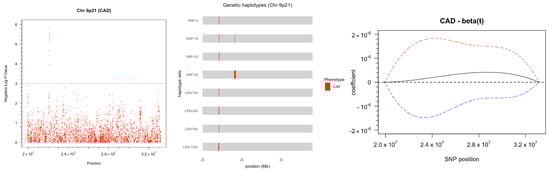
Figure 1.
(Left) Manhattan plot displaying the distribution of p-values for 3758 SNPs located on chromosome 9p21 in relation to their genomic position. (Middle) Genetic-based haplotypes constructed using a fixed number of SNPs and fixed window size that showed significant associations with CAD. (Right) Estimate and confidence bands of in functional logistic model using 3758 SNPs.

Table 1.
Single SNP tests found 9 SNPs strongly associated with CAD in chromosome 9p21 with p-value .
3.2. Genetic Haplotypes
We used two common approaches to construct the genetic-based haplotypes: (1) blocks containing a fixed number of SNPs and (2) fixed genomics window of size. In these two approaches, we have constructed blocks containing 5, 10, 20, and 50 SNPs and blocks with window sizes 10 kb, 20 kb, 50 kb, and 100 kb, respectively. It ends up with 1392 blocks generated for (1) and 2394 blocks generated for (2).
To compute the p-value of each haplotype, we fit a GLM for each haplotype while adjusting for confounding factors and compare it to a base model with only an intercept and confounding factors. However, due to missing values in our genotype data, samples containing missing values for any SNP in a haplotype were excluded when fitting the models. To ensure sufficient data for fitting GLMs, we imputed missing values using the most frequent value (mode) for each SNP before computing the p-values.
Applying the same p-value threshold of as we did for single SNP tests, we found 9 significant blocks associated with CAD using Approach (1) and 11 significant blocks using Approach (2). Figure 1 (middle) displays the positions of the significant blocks, which are primarily located around 22 Mb with a few at around 24 Mb. These findings are consistent with our results from single SNP tests, which identified significant single SNPs near 22 Mb. The haplotypes at around 24 Mb have larger p-values (>) as compared with the haplotypes at 22 Mb. Therefore, they could be considered as noise instead of true associations. Table 2 provides further details on the significant blocks, including their p-values.
Table 2.
Significant genetic haplotypes found by fixed SNP and fixed window size methods.
3.3. Two-Step FDA Approach
In the two-step approach, we construct the FDA-based haplotypes based on the functional GLM coefficients, as explained in Section 2. This involved smoothing the log-odds curves using 64 cubic spline basis functions to approximate the genotype, with the positions of the SNPs in the genome treated as the continuum t for the functions. Then, we transform the log-odds curves back to probability curves and fit the functional logistic model as described in Equation (6). In regression analysis, we used AIC to select the appropriate number of basis functions for , resulting in cubic spline basis functions with . The confidence bands of the estimated coefficient curve are displayed in Figure 1 (right). However, in a large number of SNPs, small signals in the SNPs may be overlooked. In fact, the confidence bands in Figure 1 barely found any signals in SNPs. As a result, we divided the SNPs into four chunks with an equal window size of approximately 3.3 Mb per chunk and fit the curves independently. For each chunk, the number of basis functions for SNPs was set to 64. The number of bases for in the functional logistic models of the four chunks were chosen as (), (), (), and () in the model selection. The final estimated coefficient curves and their confidence bands for all four chunks are presented in Figure 2.
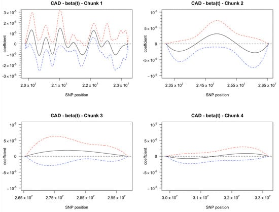
Figure 2.
Coefficient curve with its 95% confidence band. It indicates significant associations between CAD and SNPs in Chunk 1 at around position 22.1 Mb only.
The plots suggest that SNPs located around 22 Mb exhibit strong associations with the phenotype, CAD. The confidence bands indicate strong positive associations of 68 SNPs in the position range of 21986218 to 22219365 at the significance level. When the significance level is , the number of SNPs with significant associations is reduced to 62 in the position range of 21988896 to 22176961. It is worth noting that there are some weak associations between CAD and a small number of SNPs located at 19914792 to 19915135, 20028452 to 20057787, and 21747672 to 21869079. These associations are significant at significance level but not at , and therefore, are considered noises rather than signals.
4. Discussion
As stated in Section 2.1, we anticipated finding associations between SNPs in 9p21.3 and CAD. In our experiments, all three methods identified significant SNPs and haplotypes within this region (19.9 Mb to 25.6 Mb). Specifically, the SNPs with the smallest p-values in single SNP tests were located between 22.06 Mb and 22.13 Mb, while most of the strongly associated haplotypes in genetic haplotypes were found at 22.06 Mb to 22.20 Mb. Similarly, in FDA haplotypes, the most significant haplotype was found around 21.98 Mb to 22.22 Mb. Notably, in the region where these associations were detected, two genes, cyclin-dependent kinase 2A and 2B: CDKN2A (21.97 Mb to 21.99 Mb) and CDKN2B (22.00 Mb to 22.01 Mb), have been implicated in conferring risk for CAD in multiple studies [16,17,18], thus validating our findings.
5. Conclusions
In this paper, we presented a novel method for smoothing the categorical SNP data in GWAS and demonstrated its effectiveness in identifying haplotypes strongly associated with disease using the PennCATH dataset. The FDA haplotypes successfully retrieved all significant regions in the SNPs while maintaining low false-positive rates at low significance levels. Both functional and non-functional methods were successful, but the main advantage of the functional method is its ability to efficiently identify important SNPs without an exhaustive search while naturally incorporating spatial information and correlation among SNPs into the regression models. Additionally, in the presence of missing values, it implicitly imputes the missing SNP values when smoothing the curves, eliminating the need to exclude or impute missing values in SNPs. This prevents it from getting biased results when missing values are not handled correctly. There is not a large discrepancy between the curves smoothed directly by the least-square method and the curves smoothed by our novel approach. However, our approach, which considers the data as binomial probability curves, has better interpretability and resolves the issue of violating the normality assumption.
Author Contributions
Conceptualization, G.Q.; methodology, P.-Y.S. and G.Q.; software, P.-Y.S.; validation, P.-Y.S. and G.Q.; formal analysis, P.-Y.S. and G.Q.; investigation, P.-Y.S. and G.Q.; resources, P.-Y.S. and G.Q.; data curation, P.-Y.S.; writing—original draft preparation, P.-Y.S.; writing—review and editing, G.Q.; visualization, P.-Y.S.; supervision, G.Q.; project administration, P.-Y.S. and G.Q.; funding acquisition, G.Q. All authors have read and agreed to the published version of the manuscript.
Funding
This research received no external funding.
Institutional Review Board Statement
Not applicable.
Informed Consent Statement
Not applicable.
Data Availability Statement
No new data were created or analyzed in this study. Data sharing is not applicable to this article.
Acknowledgments
Pei-Yun Sun’s research in this paper was supported by the University of Melbourne Graduate Research Training Scholarship.
Conflicts of Interest
The authors declare no conflict of interest.
References
- Uffelmann, E.; Huang, Q.Q.; Munung, N.S.; de Vries, J.; Okada, Y.; Martin, A.R.; Martin, H.C.; Lappalainen, T.; Posthuma, D. Genome-wide association studies. Nat. Rev. Methods Prim. 2021, 1, 59. [Google Scholar] [CrossRef]
- Fan, R.; Wang, Y.; Mills, J.L.; Wilson, A.F.; Bailey-Wilson, J.E.; Xiong, M. Functional linear models for association analysis of quantitative traits. Genet. Epidemiol. 2013, 37, 726–742. [Google Scholar] [CrossRef] [PubMed]
- Wu, M.C.; Lee, S.; Cai, T.; Li, Y.; Boehnke, M.; Lin, X. Rare-variant association testing for sequencing data with the sequence kernel association test. Am. J. Hum. Genet. 2011, 89, 82–93. [Google Scholar] [CrossRef] [PubMed]
- Lee, S.; Emond, M.J.; Bamshad, M.J.; Barnes, K.C.; Rieder, M.J.; Nickerson, D.A.; Christiani, D.C.; Wurfel, M.M.; Lin, X.; Project, N.G.E.S.; et al. Optimal unified approach for rare-variant association testing with application to small-sample case-control whole-exome sequencing studies. Am. J. Hum. Genet. 2012, 91, 224–237. [Google Scholar] [CrossRef] [PubMed]
- Li, Y.; Wang, F.; Wu, M.; Ma, S. Integrative functional linear model for genome-wide association studies with multiple traits. Biostatistics 2022, 23, 574–590. [Google Scholar] [CrossRef] [PubMed]
- Jadhav, S.; Tong, X.; Lu, Q. A functional U-statistic method for association analysis of sequencing data. Genet. Epidemiol. 2017, 41, 636–643. [Google Scholar] [CrossRef] [PubMed]
- Chiu, C.y.; Zhang, B.; Wang, S.; Shao, J.; Lakhal-Chaieb, M.L.; Cook, R.J.; Wilson, A.F.; Bailey-Wilson, J.E.; Xiong, M.; Fan, R. Gene-based association analysis of survival traits via functional regression-based mixed effect cox models for related samples. Genet. Epidemiol. 2019, 43, 952–965. [Google Scholar] [CrossRef] [PubMed]
- Reilly, M.; Li, M.; He, J.; Ferguson, J.; Stylianou, I.; Mehta, N.; Burnett, M.; Devaney, J.; Knouff, C.; Thompson, J.; et al. Identification of ADAMTS7 as a novel locus for coronary atherosclerosis and association of ABO with myocardial infarction in the presence of coronary atherosclerosis: Two genome-wide association studies. Lancet 2011, 377, 383–392. [Google Scholar] [CrossRef] [PubMed]
- Reed, E.; Nunez, S.; Kulp, D.; Qian, J.; Reilly, M.P.; Foulkes, A.S. A guide to genome-wide association analysis and post-analytic interrogation. Stat. Med. 2015, 34, 3769–3792. [Google Scholar] [CrossRef] [PubMed]
- Jarinova, O.; Stewart, A.F.; Roberts, R.; Wells, G.; Lau, P.; Naing, T.; Buerki, C.; McLean, B.W.; Cook, R.C.; Parker, J.S.; et al. Functional analysis of the chromosome 9p21. 3 coronary artery disease risk locus. Arterioscler. Thromb. Vasc. Biol. 2009, 29, 1671–1677. [Google Scholar] [CrossRef] [PubMed]
- Shen, G.Q.; Li, L.; Rao, S.; Abdullah, K.G.; Ban, J.M.; Lee, B.S.; Park, J.E.; Wang, Q.K. Four SNPs on chromosome 9p21 in a South Korean population implicate a genetic locus that confers high cross-race risk for development of coronary artery disease. Arterioscler. Thromb. Vasc. Biol. 2008, 28, 360–365. [Google Scholar] [CrossRef] [PubMed]
- Chen, Z.; Qian, Q.; Ma, G.; Wang, J.; Zhang, X.; Feng, Y.; Shen, C.; Yao, Y. A common variant on chromosome 9p21 affects the risk of early-onset coronary artery disease. Mol. Biol. Rep. 2009, 36, 889. [Google Scholar] [CrossRef] [PubMed]
- Edwards, A. Anecdotal, Historical and Critical Commentaries on Genetics: GH Hardy (1908) and Hardy–Weinberg Equilibrium. Genetics 2008, 179, 1143. [Google Scholar] [CrossRef] [PubMed]
- Turner, S.; Armstrong, L.L.; Bradford, Y.; Carlson, C.S.; Crawford, D.C.; Crenshaw, A.T.; De Andrade, M.; Doheny, K.F.; Haines, J.L.; Hayes, G.; et al. Quality control procedures for genome-wide association studies. Curr. Protoc. Hum. Genet. 2011, 68, 1–19. [Google Scholar] [CrossRef] [PubMed]
- Marees, A.T.; de Kluiver, H.; Stringer, S.; Vorspan, F.; Curis, E.; Marie-Claire, C.; Derks, E.M. A tutorial on conducting genome-wide association studies: Quality control and statistical analysis. Int. J. Methods Psychiatr. Res. 2018, 27, e1608. [Google Scholar] [CrossRef] [PubMed]
- Almontashiri, N.A. The 9p21. 3 risk locus for coronary artery disease: A 10-year search for its mechanism. J. Taibah Univ. Med. Sci. 2017, 12, 199–204. [Google Scholar] [PubMed]
- McPherson, R.; Pertsemlidis, A.; Kavaslar, N.; Stewart, A.; Roberts, R.; Cox, D.R.; Hinds, D.A.; Pennacchio, L.A.; Tybjaerg-Hansen, A.; Folsom, A.R.; et al. A common allele on chromosome 9 associated with coronary heart disease. Science 2007, 316, 1488–1491. [Google Scholar] [CrossRef] [PubMed]
- Zhong, J.; Chen, X.; Ye, H.; Wu, N.; Chen, X.; Duan, S. CDKN2A and CDKN2B methylation in coronary heart disease cases and controls. Exp. Ther. Med. 2017, 14, 6093–6098. [Google Scholar] [CrossRef]
Disclaimer/Publisher’s Note: The statements, opinions and data contained in all publications are solely those of the individual author(s) and contributor(s) and not of MDPI and/or the editor(s). MDPI and/or the editor(s) disclaim responsibility for any injury to people or property resulting from any ideas, methods, instructions or products referred to in the content. |
© 2023 by the authors. Licensee MDPI, Basel, Switzerland. This article is an open access article distributed under the terms and conditions of the Creative Commons Attribution (CC BY) license (https://creativecommons.org/licenses/by/4.0/).