Proceeding Paper

A Multi-Fidelity Deep Neural Network Approach to Structural Health Monitoring †

1
Dipartimento di Ingegneria Civile e Ambientale, Politecnico di Milano, Piazza L. da Vinci 32, 20133 Milano, Italy
2
MOX, Dipartimento di Matematica, Politecnico di Milano, Piazza L. da Vinci 32, 20133 Milano, Italy
*
Author to whom correspondence should be addressed.
Presented at the 9th International Electronic Conference on Sensors and Applications, 1–15 November 2022; Available online: https://ecsa-9.sciforum.net/.
Eng. Proc. 2022, 27(1), 60; https://doi.org/10.3390/ecsa-9-13344
Published: 1 November 2022

Abstract

:
The structural health monitoring (SHM) of civil structures and infrastructures is becoming a crucial issue in our smart and hyper-connected age. Due to structural aging and to unexpected loading conditions, partially linked to extreme events caused by the climate change, reliable and real-time SHM schemes are currently facing a burst in development and applications. In this work, we propose a procedure that relies upon a surrogate modeling scheme based on a multi-fidelity (MF) deep neural network (DNN), which has been conceived to sense and identify a structural damage under operational (and possibly environmental) variability. By exploiting the sensor recordings from a densely deployed network within a fully stochastic framework, the MF-DNN model is adopted to feed a Markov chain Monte Carlo (MCMC) sampling procedure and update the probability distribution of the structural state, conditioned on noisy observations. As information regarding the health of real structures is usually rather limited, the datasets to train the MF-DNN are generated with physical (e.g., finite element) models: high-fidelity (HF) and low-fidelity (LF) models are adopted to simulate the structural response under the mentioned varying conditions, respectively, in the presence or absence of a structural damage. As far as the architecture of the DNN is concerned, the MF approach is obtained by merging a fully connected LF-DNN and a long short-term memory HF-DNN. The LF-DNN mimics the output of the sensor network in the undamaged condition, while the HF-DNN is exploited to improve the LF model and appropriately catch the structural response in the presence of a pre-defined set of damaged patterns. Thanks to the adaptive enrichment of the LF signals carried out by the MF-DNN, the proposed model updating strategy is reported capable of locating (and possibly quantifying) a damage event.

1. Introduction

In civil engineering, numerical models are often used to approximate the structural response of real-life structures, accounting also for uncertainties related to their geometrical and material properties. Within this field, a relevant challenge concerns the optimal management of deteriorating structural systems. The evolution from classical time-based maintenance practices with scheduled inspections toward condition-based ones has been recently put forth, to increase the system safety and availability at the same time [1,2]. This is made possible by permanent data collecting systems and by diagnostic activities, to feed a digital twin of the structural system. SHM has thus become a standard and widespread framework for the identification of damage inception and evolution under varying loading conditions. Vibration-based SHM techniques exploit dynamic response data collected by a sensor network, to assess the damage; this perspective looks therefore well suited for an automated monitoring and to substitute non-destructive tests [3,4].
Approaches to SHM can be classified as either data-driven [5,6,7,8] or model-based [9,10]: the former, which is the one we focus on in this work, exploits the data to dig into the relationship between the structural response, in terms of, e.g., selected features, and the damage pattern to be identified [11,12]; the latter exploits instead physics-based numerical models to assess the damage via model updating [13]. To deal with uncertainties in a proper way and sampling solutions from the relevant probability density functions (pdfs), MCMC methods are frequently adopted [14,15]. Such procedures can incur in high computational costs, mainly linked to repeated evaluations of the nunerical model they rely upon, thus preventing real-time applications. The computational efficiency can be improved by replacing computationally demanding numerical models with data-driven surrogate models, obsersve, e.g., [16,17,18,19]. In the case of multiple models available to simulate the structural response with a different accuracy, namely in case of a MF framework, the simultaneous use of LF and HF model responses can provide a reduction of the overall computational burden, also keeping a selective accuracy of the global output high enough to allow the localization and quantification of damage.
Along the aforementioned research line, in this work we propose a MF-DNN surrogate model, observe, e.g., [20,21]. Such a model is characterized by a multi-level architecture based on two DNNs, which are, respectively, the LF and HF parts of the entire model. A fully-connected DNN is used to mimic sensor recordings in the undamaged structural state, whilst a long short-term memory (LSTM)-based model is used to approximate the effect of damage on the structural response. The two DNNs are trained on data related to the vibration responses, within a simulation-based paradigm. The performance of the proposed method is assessed on a L-shaped cantilever beam, to obtain insights into its accuracy and efficiency.

2. MF-DNN Surrogate Modeling

As already pointed out, the LF and HF datasets D LF and D HF , respectively, collect the structural responses in the absence and presence of the damage. As customarily assumed, the initial SHM phase refers to the undamaged state. Datasets D LF and D HF consist of I LF and I HF < I LF instances, so that:
D LF = { ( x i LF , U i LF ) } i = 1 I LF , D HF = { ( x j HF , U j HF ) } j = 1 I HF ,
where: x i LF R N par LF represents the operational conditions inducing the LF vibration recordings U i LF ( x i LF ) = [ u 1 LF , , u N u LF ] i R N u × L ; the N u time series are assumed made of L measurements in the time interval ( 0 , T ) ; the damage is accounted for in the HF recordings U j HF ( x j HF ) = [ u 1 HF , , u N u HF ] j R N u × L ; the N par HF input parameters x j HF R N par HF control instead the operational and the damage conditions in the current state.
The HF model describes the dynamic response of the structure under the applied loadings, assuming a linearized kinematic. The semi-discretized equations of the motion thus read:
M HF d ¨ HF ( t ) + C HF ( x HF ) d ˙ HF ( t ) + K HF ( x HF ) d HF ( t ) = f HF ( t , x HF ) ,
to be supplemented by the relevant initial conditions d HF ( 0 ) = d 0 HF and d ˙ HF ( 0 ) = d ˙ 0 HF in terms of nodal displacements and velocities, respectively. Here: t ( 0 , T ) denotes time; d HF ( t ) , d ˙ HF ( t ) , d ¨ HF R M are the vectors of nodal displacements, velocities and accelerations; M is the number of system degrees of freedom (dofs); M HF R M × M is the mass matrix; C HF ( x HF ) R M × M is the damping matrix; K HF ( x HF ) R M × M is the stiffness matrix; f HF ( t , x HF ) R M is the vector of external forces.
The structural damage is modeled as a localized degradation of the material stiffness, which is dealt with by means of a parametrization of the stiffness matrix K HF through the variables y R 3 and δ R , collected in x HF , that denote position and magnitude of the stiffness reduction.
The considered LF model is a projection-based reduced order model (ROM) of the HF one, observe, e.g., [22,23,24], obtained by linearly combining M LF M proper orthogonal decomposition (POD) basis functions w k R M , k = 1 , , M LF , as d LF ( t , x LF ) W r ( t , x LF ) , where W = [ w 1 , , w M LF ] R M × M LF is the projection matrix and r ( t , x LF ) R M LF are the unknown POD coefficients. The following M LF -dimensional ROM is so obtained:
M r r ¨ ( t ) + K r r ( t ) = f r ( t , x LF ) ,
wherein the damping effects are disregarded, and:
M r W M HF W , K r W K LF W , f r ( t , x LF ) W f HF ( t , x LF ) ,
with the projection matrix W obtained with the so-called method of snapshots.
To set the entries of D LF and D HF , x LF and x HF are assumed to be uniformly distributed within their input spaces. The instances are generated by sampling x LF and x HF via latin hypercube rule and picking up the measurables from the system state vectors through appropriate Boolean operations.
Moving on to the deep learning stage of the procedure, the MF-DNN surrogate NN MF is composed as well of the LF and HF parts, respectively termed NN LF and NN HF . NN LF is a fully-connected DNN used to mimic the vibration recordings for any given LF input data x LF , according to:
U ^ LF ( x LF ) = vec N u × L 1 [ Y ( 1 ω NN LF ( x LF ) ) ] , NN LF ( x LF ) = ω h ^ ( x LF ) ,
where: vec : R m × n R m n denotes the vectorization operation, and vec m × n 1 : R m n R m × n is its inverse; Y = [ y 1 , , y L LF ] R L concat × L LF , with L concat = L N u , is a matrix of L LF L concat POD basis functions used to reduce the number of trainable parameters of NN LF ; R L LF h ( x LF ) = [ h 1 ( x LF ) , , h L LF ( x LF ) ] = Y vec [ U LF ] are the POD coefficients; ⊙ is the Hadamard product; ω R L LF is a vector used to weight the relative importance of the POD basis functions.
NN LF is a 9-layers fully-connected DNN with residual connections. All layers feature 30 neurons, except the last two that are equipped with 2 L LF and L LF neurons, respectively. A couple of double-layer identity residual connections [25] are also exploited, to perform an iterative refinement of the outcome. No activation is used for the last layer, while the PReLU [26] one is employed elsewhere. During training, the weights Ω LF are tuned by minimizing the following loss function:
L LF ( Ω LF , D LF ) = 1 I LF i = 1 I LF 1 L LF ω ( Y vec [ U i LF ] ) NN LF ( x i LF ) 2 2 + λ LF Ω LF 2 2 ,
where λ LF plays the role of a regularization parameter. The loss function is minimized using the Adam algorithm for a maximum of 10,000 allowed epochs. The learning rate η LF is initially set to 0.005 , and decreased for 4 / 5 of the allowed training steps using a cosine decay schedule with weight decay equal to 0.02 . An early-stopping strategy is used to interrupt the learning process, whenever overfitting shows up.
NN HF is instead built upon the LSTM scheme, that is used to mimic the time correlation between the two fidelity levels. Recurrent neural networks (RNNs), such as the adopted LSTM one, can handle the sequences of the inputs of variable length thanks to a hidden state variable that acts as a data memory. As RNNs can fail in addressing long-term dependencies due to the vanishing/exploding gradients issue arising during the back propagation through time [27], the LSTM cell model [28] can better capture long-term dependencies by means of an internal gating mechanism [27]. The NN HF consists of four LSTM layers, with cell states of size 16 , 16 , 32 , N u , and of a time distributed fully-connected output layer with N u neurons. No activation is applied to the dense layer, while the LSTM layers have standard cells with sigmoidal gating functions and hyperbolic tangent activated states. The weights Ω HF are tuned by minimizing the following loss function:
L HF ( Ω HF , D HF ) = 1 I HF 1 N C j = 1 I HF τ = 1 N C 1 N u 1 L C vec [ U j , τ : τ + L C HF NN HF ( x j HF , U ^ τ : τ + L C LF ( x LF ( x j HF ) ) , t τ : τ + L C ) ] 1 + λ HF Ω HF 2 2 .
The optimization is carried out by using the Adam algorithm again. The learning rate is decreased as the training advances using a cosine decay schedule, and an early stopping strategy is adopted to prevent overfitting issues.

3. Results

To assess the performance of the proposed MF-DNN surrogate model, the cantilever beam depicted in Figure 1 is considered. The structure is made of two arms having a length of 4 m , a width of 0.3 m and a height of 0.4 m . The structure is assumed to be made of concrete, with mechanical properties: Young’s modulus E = 30 G P a , Poisson’s ratio ν = 0.2 , density ρ = 2500 k g / m 3 . The structure is excited by a distributed vertical load q ( t ) , acting on an area of ( 0.3 × 0.3 ) m 2 close to the beam tip and varying according to q ( t ) = Q sin ( 2 π f t ) , with Q [ 1 , 5 ] k P a and f [ 10 , 60 ] H z being the load amplitude and frequency. We assume that f and Q are uniformly distributed in their ranges.
Displacement time histories U LF ( x LF ) = [ u 1 LF , , u N u LF ] and U HF ( x HF ) = [ u 1 HF , , u N u HF ] are recorded from N u = 8 sensors placed along the bottom surface of the structure. The recordings are provided for the time interval ( 0 , T = 1 s ) with a 200 H z sampling rate. The HF numerical model is obtained from a finite element discretization using linear tetrahedral elements and resulting in M = 4659 dofs. Damage is simulated via a 25 % reduction of the material stiffness within a subdomain Ω y , whose size is ( 0.3 × 0.3 × 0.4 ) m 3 , and whose position is parametrized by the coordinates of its center of mass y = ( x Ω , y Ω ) , with x Ω , y Ω [ 0.15 , 3.85 ] m . The ROM is obtained by prescribing a high accuracy, so that its order is set to M LF = 14 , leading to a speed-up in the analyses of about 25.8 times. I LF = 10,000 LF instances are collected to train NN LF , while only I HF = 1000 additional HF instances are exploited to train NN HF .
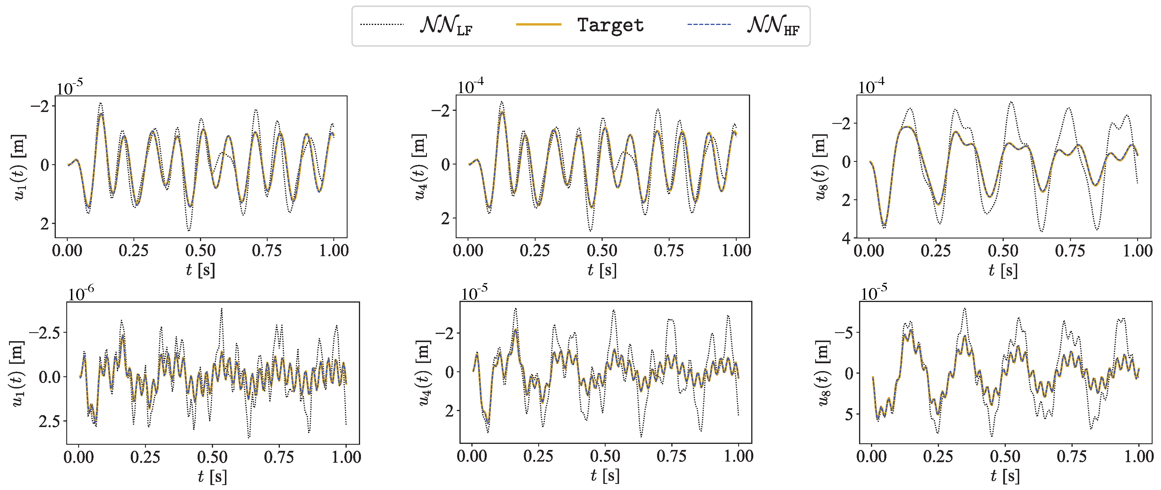
To show the capabilities of the surrogate model to match the ground truth solution, some exemplary signals provided by NN MF are reported in Figure 2, together with the corresponding LF approximations and target signals, at varying input parameters. It can be observed that the NN MF model always match very well the target signal, in relation to both the low and high frequency components. Though not shown, preventing NN HF from exploiting the correlation between HF and LF recordings spoils the approximation capabilities of NN MF , as NN LF seems to play a crucial role in helping NN HF to maintain correct solutions in time. Intuitively, this loss of accuracy is due to the fact that, if NN LF is removed, NN HF needs to learn not only how to enrich the LF signals with the effects of damage and structural damping but to reproduce the entire input–output behavior.

4. Conclusions

In this work, we have proposed a strategy to build MF surrogate models for structural health monitoring in a non-intrusive way, exploiting DNNs. The framework allows to map damage and operational parameters onto recordings linked to the structural response to the external loading. The modeling scheme is based on a two-level architecture, characterized by the relevant DNNs to be trained separately: a fully-connected model is used to mimic sensor recordings in the undamaged state; a long short-term memory model is used to enrich the approximation with the effect of damage. The effects of damage are accounted for without the need of model order reduction techniques, prone to losing damage-sensitive components.
The strategy has been tested against a cantilever beam, and the results have demonstrated that a (structure-independent) remarkable accuracy can be obtained. Though not shown, it has also outperformed the single-fidelity counterpart in mimicking the structural response. The computing time to obtain results from the surrogate model has been demonstrated to be up to three orders of magnitude smaller than that corresponding to the full-order model.
In future activities, the capability of the strategy will be assessed while feeding MCMC algorithms empowered by a Siamese DNN, allowing for measurement noise and varying operational conditions. Some preliminary results have demonstrated that learnable features used in place of the raw vibration recordings would enable improvements in the parameter identification outcomes, especially in terms of damage detection and localization.

Author Contributions

Conceptualization, M.T., A.M. and S.M.; methodology, M.T., A.M. and S.M.; software, M.T.; validation, M.T., A.M. and S.M.; formal analysis, M.T., A.M. and S.M.; investigation, M.T.; resources, A.M. and S.M.; data curation, M.T.; writing—original draft preparation, M.T.; writing—review and editing, M.T., A.M. and S.M.; visualization, M.T.; supervision, A.M. and S.M.; project administration, A.M. and S.M.; funding acquisition, A.M. and S.M. All authors have read and agreed to the published version of the manuscript.

Funding

This research received no external funding.

Institutional Review Board Statement

Not applicable.

Informed Consent Statement

Not applicable.

Data Availability Statement

Not applicable.

Acknowledgments

M.T. acknowledges the financial support by Politecnico di Milano through the interdisciplinary Ph.D. Grant “Physics-Informed Deep Learning for Structural Health Monitoring”.

Conflicts of Interest

The authors declare no conflict of interest.

References

  1. Farrar, C.; Worden, K. Structural Health Monitoring A Machine Learning Perspective; Wiley: Chichester, UK, 2013. [Google Scholar] [CrossRef] [Green Version]
  2. Neves, A.C.; Gonzalez, I.; Karoumi, R. Development and Validation of a Data-Based SHM Method for Railway Bridges. In Structural Health Monitoring Based on Data Science Techniques; Springer International Publishing: Cham, Switzerland, 2022; pp. 95–116. [Google Scholar] [CrossRef]
  3. Rosafalco, L.; Torzoni, M.; Manzoni, A.; Mariani, S.; Corigliano, A. A Self-adaptive Hybrid Model/data-Driven Approach to SHM Based on Model Order Reduction and Deep Learning. In Structural Health Monitoring Based on Data Science Techniques; Springer International Publishing: Cham, Switzerland, 2022; pp. 165–184. [Google Scholar] [CrossRef]
  4. García-Macías, E.; Ubertini, F. Integrated SHM Systems: Damage Detection Through Unsupervised Learning and Data Fusion. In Structural Health Monitoring Based on Data Science Techniques; Springer International Publishing: Cham, Switzerland, 2022; pp. 247–268. [Google Scholar] [CrossRef]
  5. Torzoni, M.; Manzoni, A.; Mariani, S. Structural health monitoring of civil structures: A diagnostic framework powered by deep metric learning. Comput. Struct. 2022, 271, 106858. [Google Scholar] [CrossRef]
  6. Worden, K. Structural fault detection using a novelty measure. J. Sound. Vib. 1997, 201, 85–101. [Google Scholar] [CrossRef]
  7. Rosafalco, L.; Manzoni, A.; Mariani, S.; Corigliano, A. Fully convolutional networks for structural health monitoring through multivariate time series classification. Adv. Model. Simul. Eng. Sci. 2020, 7, 38. [Google Scholar] [CrossRef]
  8. Entezami, A.; Sarmadi, H.; Behkamal, B.; Mariani, S. Big data analytics and structural health monitoring: A statistical pattern recognition-based approach. Sensors 2020, 20, 2328. [Google Scholar] [CrossRef] [PubMed] [Green Version]
  9. Kamariotis, A.; Chatzi, E.; Straub, D. Value of information from vibration-based structural health monitoring extracted via Bayesian model updating. Mech. Syst. Signal. Process. 2022, 166, 108465. [Google Scholar] [CrossRef]
  10. Eftekhar Azam, S.; Mariani, S. Online damage detection in structural systems via dynamic inverse analysis: A recursive Bayesian approach. Eng. Struct. 2018, 159, 28–45. [Google Scholar] [CrossRef]
  11. Bishop, C.M. Pattern Recognition and Machine Learning (Information Science and Statistics); Springer: New York, NY, USA, 2006. [Google Scholar]
  12. Avci, O.; Abdeljaber, O.; Kiranyaz, S.; Hussein, M.; Gabbouj, M.; Inman, D. A review of vibration-based damage detection in civil structures: From traditional methods to Machine Learning and Deep Learning applications. Mech. Syst. Signal. Process. 2021, 147, 107077. [Google Scholar] [CrossRef]
  13. Warner, J.; Zubair, M.; Ranjan, D. Near real time damage diagnosis using surrogate modeling and high performance computing. In Proceedings of the 19th AIAA Non-Deterministic Approaches Conference, Grapevine, TX, USA, 9–13 January 2017; p. 1563. [Google Scholar] [CrossRef]
  14. Hou, R.; Wang, X.; Xia, Y. Vibration-Based Structural Damage Detection Using Sparse Bayesian Learning Techniques. In Structural Health Monitoring Based on Data Science Techniques; Springer International Publishing: Cham, Switzerland, 2022; pp. 1–25. [Google Scholar] [CrossRef]
  15. Green, P.L.; Worden, K. Bayesian and Markov chain Monte Carlo methods for identifying nonlinear systems in the presence of uncertainty. Philos. Trans. R. Soc. A 2015, 373, 20140405. [Google Scholar] [CrossRef] [PubMed] [Green Version]
  16. Mirzazadeh, R.; Eftekhar Azam, S.; Mariani, S. Mechanical characterization of polysilicon MEMS: A hybrid TMCMC/POD-kriging approach. Sensors 2018, 18, 1243. [Google Scholar] [CrossRef] [PubMed] [Green Version]
  17. Rocchetta, R.; Broggi, M.; Huchet, Q.; Patelli, E. On-line Bayesian model updating for structural health monitoring. Mech. Syst. Signal Process. 2018, 103, 174–195. [Google Scholar] [CrossRef]
  18. Meeds, E.; Welling, M. GPS-ABC: Gaussian process surrogate approximate Bayesian computation. arXiv 2014, arXiv:1401.2838. [Google Scholar]
  19. García-Macías, E.; Ierimonti, L.; Venanzi, I.; Ubertini, F. An innovative methodology for online surrogate-based model updating of historic buildings using monitoring data. Int. J. Archit. Herit. 2021, 15, 92–112. [Google Scholar] [CrossRef]
  20. Meng, X.; Babaee, H.; Karniadakis, G.E. Multi-fidelity Bayesian Neural Networks: Algorithms and Applications. J. Comput. Phys. 2021, 438, 110361. [Google Scholar] [CrossRef]
  21. Guo, M.; Manzoni, A.; Amendt, M.; Conti, P.; Hesthaven, J. Multi-fidelity regression using artificial neural networks: Efficient approximation of parameter-dependent output quantities. Comput. Methods Appl. Mech. Eng. 2022, 389, 114378. [Google Scholar] [CrossRef]
  22. Rosafalco, L.; Manzoni, A.; Mariani, S.; Corigliano, A. Combined Model Order Reduction Techniques and Artificial Neural Network for Data Assimilation and Damage Detection in Structures. In Computational Sciences and Artificial Intelligence in Industry: New Digital Technologies for Solving Future Societal and Economical Challenges; Springer International Publishing: Cham, Switzerland, 2022; pp. 247–259. [Google Scholar] [CrossRef]
  23. Rosafalco, L.; Torzoni, M.; Manzoni, A.; Mariani, S.; Corigliano, A. Online structural health monitoring by model order reduction and deep learning algorithms. Comput. Struct. 2021, 255, 106604. [Google Scholar] [CrossRef]
  24. Torzoni, M.; Rosafalco, L.; Manzoni, A.; Mariani, S.; Corigliano, A. SHM under varying environmental conditions: An approach based on model order reduction and deep learning. Comput. Struct. 2022, 266, 106790. [Google Scholar] [CrossRef]
  25. He, K.; Zhang, X.; Ren, S.; Sun, J. Deep residual learning for image recognition. In Proceedings of the IEEE Conference on Computer Vision and Pattern Recognition, Las Vegas, NV, USA, 27–30 June 2016; pp. 770–778. [Google Scholar] [CrossRef] [Green Version]
  26. He, K.; Zhang, X.; Ren, S.; Sun, J. Delving Deep into Rectifiers: Surpassing Human-Level Performance on ImageNet Classification. In Proceedings of the IEEE International Conference on Computer Vision (ICCV), Santiago, Chile, 7–13 December 2015; pp. 1026–1034. [Google Scholar] [CrossRef] [Green Version]
  27. Goodfellow, I.; Bengio, Y.; Courville, A. Deep Learning; MIT Press: Cambridge, MA, USA; London, UK, 2016. [Google Scholar]
  28. Hochreiter, S.; Schmidhuber, J. Long short-term memory. Neural Comput. 1997, 9, 1735–1780. [Google Scholar] [CrossRef] [PubMed]
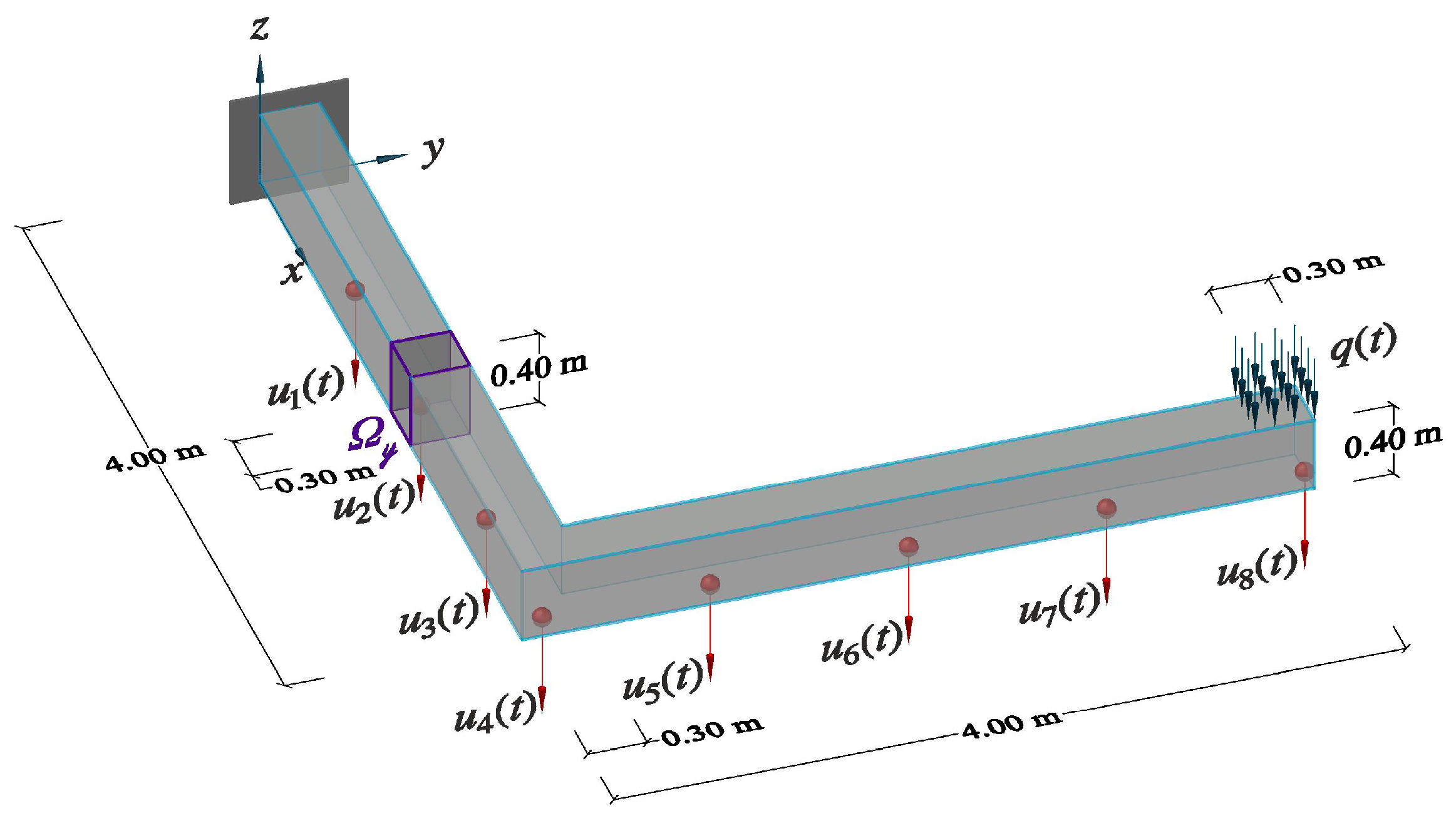
Figure 1. Cantilever beam: geometry, loading condition, damaged area Ω y , and synthetic recordings related to displacements u 1 ( t ) , , u 8 ( t ) .
Engproc 27 00060 g001
Figure 2. Cantilever beam: exemplary comparisons of u 1 ( t ) , u 4 ( t ) and u 8 ( t ) displacement time histories provided by NN LF and NN HF , with the target signals.
Engproc 27 00060 g002
Publisher’s Note: MDPI stays neutral with regard to jurisdictional claims in published maps and institutional affiliations.