Proceeding Paper

Understanding the Behavior of Gas Sensors Using Explainable AI †

by
Sanghamitra Chakraborty
*,
Simon Mittermaier
and
Cecilia Carbonelli
Infineon Technologies AG Munich, 85579 Neubiberg, Germany
*
Author to whom correspondence should be addressed.
Presented at the 9th International Electronic Conference on Sensors and Applications, 1–15 November 2022; Available online: https://ecsa-9.sciforum.net/.
Eng. Proc. 2022, 27(1), 61; https://doi.org/10.3390/ecsa-9-13350
Published: 1 November 2022

Abstract

:
Exposure to pollutants like ozone and nitrogen dioxide gas can cause serious health issues and harm the environment. Therefore, the interest in air quality and its impact on health and well-being has been steadily increasing over the years, making low-cost gas sensing devices combined with artificial intelligence (AI) increasingly popular due to their flexibility and small form factor. While AI provides state-of-the-art performance, it makes the system less transparent and more difficult to trust its decisions. With the aid of three different approaches, this paper seeks to understand and explain the predictions made by complex models for gas sensors. The use of such techniques can increase our confidence in the AI systems embedded in our products in terms of fairness, or impartiality, and robustness, or reliability. This also improves our understanding of sensor behavior and provides a more robust explanation for algorithmic choices.

1. Introduction

The increasing quantity of air pollutants such as ozone (O3) and nitrogen dioxide (NO2) poses a serious threat to humans, animals, and plants in today’s world, and, therefore, it has become necessary to monitor these pollutant levels. Recently, low-cost gas sensors with graphene as the primary material have gained popularity to detect such pollutants owing to their properties of good adsorption of gas molecules, low power consumption, and low costs [1,2]. The graphene sensor under study consists of four sensing fields functionalized with different additional materials to trigger different chemical interactions between the sensor and the target gases. Gas molecules absorbed by the graphene sheet can have an influence on its electrical conductance, making it possible to use resistance a as sensor signal. To avoid the potential saturation of graphene with gas molecules still on the surface, the sensor is heated to a high temperature periodically to accelerate desorption. Our application employs a recurrent neural network, namely a gated recurrent unit (GRU) network [3], to estimate the concentrations of O3 and NO2 in parts per billion (ppb) using the features extracted from raw signals.
While artificial intelligence has gained significant traction over the years [4,5], the question of whether we can trust such sophisticated models owing to their lack of transparency persists. In recent years, many researchers have been developing novel methods to make models more interpretable and explainable [6,7,8]. Methods such as LIME (Local Interpretable Model-Agnostic Explanations) [9] have emerged to explain the predictions made by these models. Our paper uses three approaches to make our model reliable and trustworthy. These approaches helped us understand and improve sensor behavior, and, at the same time, develop a more robust model.
The first approach is the Shapley additive explanations (SHAP) method, which ranks features in order of their importance. This method was developed by Lundberg and Lee [10] and has been recently used in a variety of research, including finance [11] and healthcare [12]. The second method is to understand the internal architecture of our GRU network. This approach is highly inspired by the works of Karparthy et al. [13] on visualizing recurrent networks for text processing and Tang et al. [14] on memory visualization in speech recognition. The third approach aims to quantify the uncertainty of predictions made by our neural network by applying techniques from Bayesian deep learning [15]. Both aleatoric and epistemic uncertainty are quantified and their meaning for the gas sensor is interpreted.

2. Methods and Results

2.1. SHAP Method

SHAP analysis estimates the individual contribution of each input feature to the overall prediction output using Shapley values [16]. The features are then ranked according to their contributions, with the highest estimates contributing more to model decisions and the lowest estimates indicating either that the features should be removed from the model or that more research is needed to raise their quality. The SHAP method is capable of calculating both local and global feature importance, where the former calculates the SHAP values of each of the data points and the latter determines the SHAP values for all data points and then averages the absolute values obtained [17]. We conducted our experiment to determine global importance, and for this, 20 features were extracted (36 features for the initial analysis which includes higher-order harmonics, see Figure 1), namely the relative resistances, R0, R1, R2, and R3, of the four sensing fields and their corresponding first-order derivatives, amplitudes, phases, and total harmonic distortion [18].

2.2. Results for SHAP Analysis

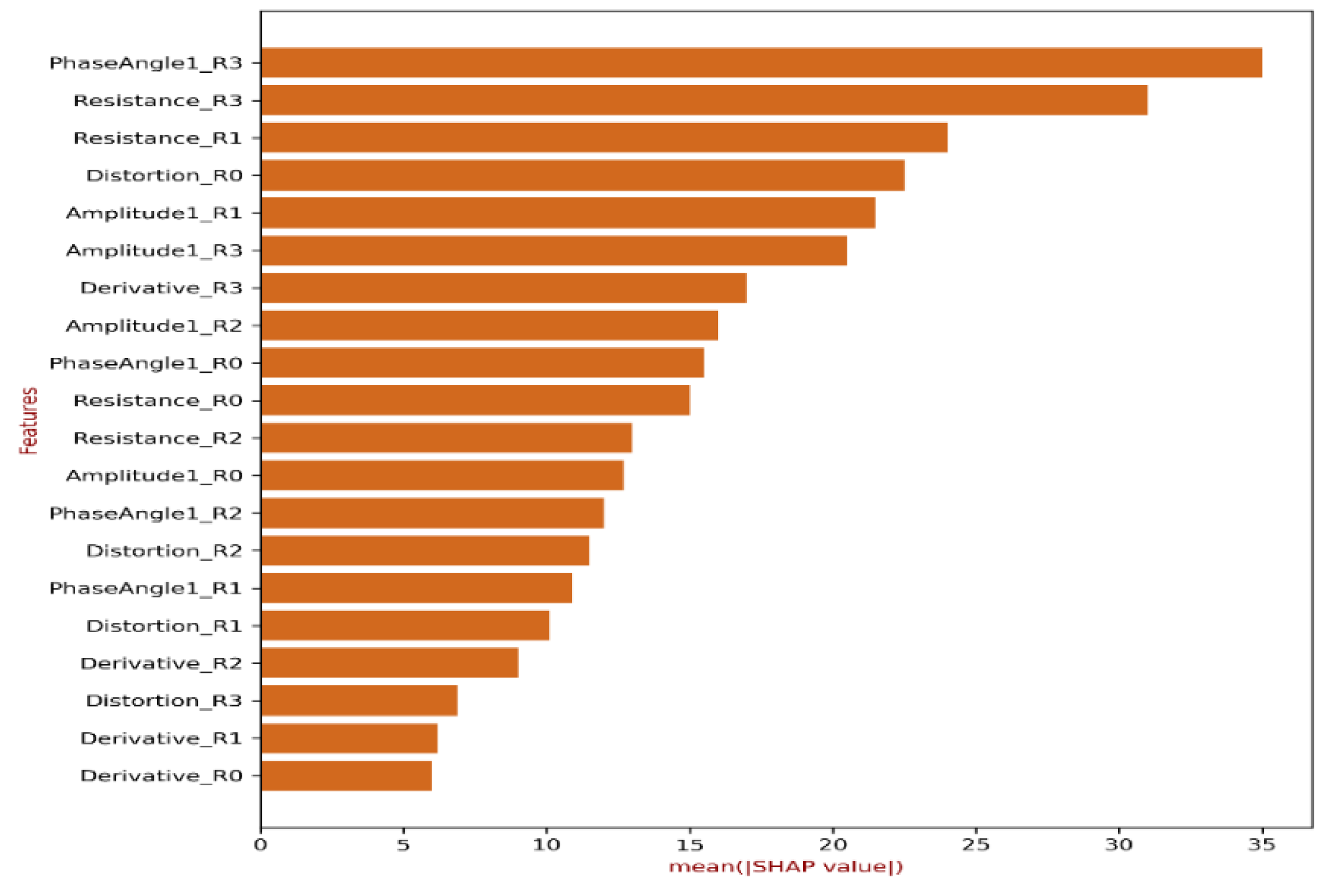
The feature ranking plot is shown in Figure 1, where the features are ordered in decreasing order of importance. Figure 1 shows R1 and its corresponding amplitude of the first harmonic having the highest contributions and R3 and its corresponding features having the least importance in the predictions despite the fact that R3 is assumed to be a very significant feature, since additional R3 characteristics such as derivatives and frequency features are extracted from this core feature. Based on this analysis, the material of the fourth sensing field (R3) was improved, and, as a result, it became one of the most stable fields in our sensor array. This can be seen in Figure 2, where the phase angle and relative resistance of this sensing field have the highest contributions to the predictions. Moreover, as seen in Figure 1, SHAP analysis revealed that the features with higher-order (second and third) harmonics had little contributions to the predictions. This allowed us to remove these features, as shown in Figure 2, thereby allowing us to build a model that is both smaller and more efficient.

2.3. Network Dissection

When using neural networks for predictions, we know the inputs and the outputs. However, we are not aware of what happens internally that makes such models reach specific decisions. This makes it challenging to understand why a certain prediction did not meet our expectations. Our research aimed to address this issue by inspecting the network’s inner architecture. As we employed GRU for the predictions in our application, we investigated its internal structure by examining the hidden state output of each GRU unit. As each unit reacts differently to each of the gases and their concentration levels, the goal is to understand which units are in charge of predicting when one gas is in the absence of another, when both gases are not present, or when there is a mixture of both in the air. It is akin to reverse engineering in the sense that we first view the output layer and then analyze the hidden layer(s) based on the outcome of the output layer. Due to the inclusion of the tanh function in each candidate hidden state, which causes the output of each hidden state to range from −1 (negative activation) to 1 (positive activation) [19], we formed two clusters, placing all positive activations in one and all negative activations in the other.

2.4. Results for Network Dissection

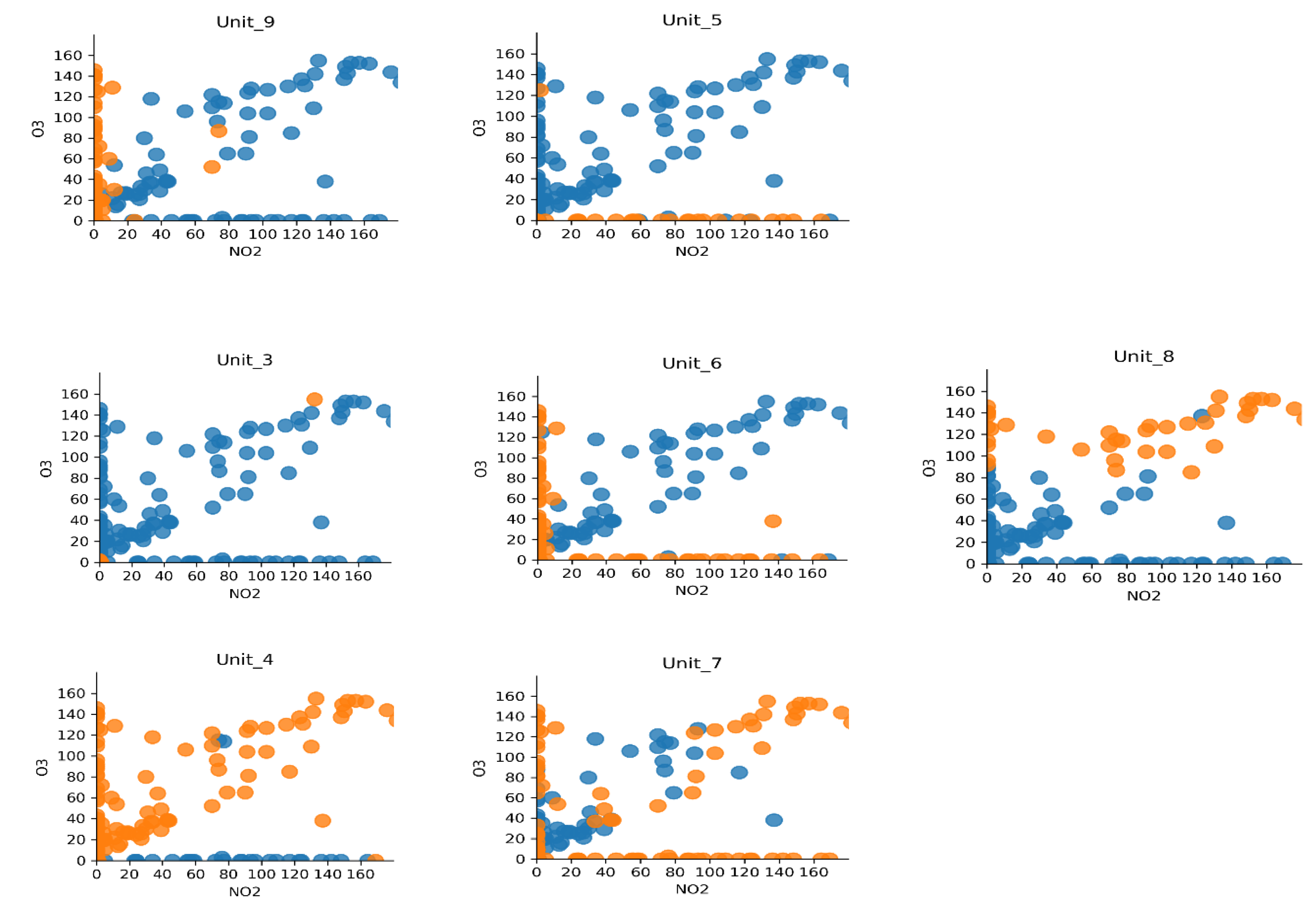
As shown in Figure 3, when there is almost no NO2, the activations of unit 9 are positive (orange points), otherwise negative (blue points), whereas unit 5 shows positive activations when there is no O3. Unit 3 is responsible for identifying the scenarios when both gases are absent, in which case the activations are positive, and when both gases are present, in which case the activations are negative. When either of the two gases is absent, unit 6 shows positive activations, otherwise negative. Unit 8 shows the patterns of when there is a mixture of both gases, where the activations are negative when O3 is below 90 ppb and positive when above. In unit 4, for a combination of no O3 and NO2 approximately above 8 ppb, the activations are negative, but as O3 increases these become positive. No unit showed such a pattern when there is a gradual increase in NO2; this confirms that as O3 increases, NO2 slowly gets overshadowed by the model. This investigation confirms the general observation that chemical sensors typically struggle to detect NO2 when O3 concentrations are higher. Moreover, not all the units demonstrated a human-level understanding, as in the case of unit 7.
This analysis was also done with fewer units in the beginning, but it was difficult to make any interpretations because the patterns were not clearly distinguishable. This also sheds some light on hyperparameters optimization, such as choosing the right number of units by understanding the network’s behavior instead of simply using a heuristic approach.

2.5. Bayesian Deep Learning

Having now analyzed how input features impact model decisions via SHAP analysis and having visualized the internal workings of the network via network dissection, techniques of Bayesian deep learning can help us to provide a more interpretable and reliable output with our model by quantifying its uncertainty. Many applications require accurate yet reliable and trustworthy predictions. However, machine learning models are often over- or underconfident in their predictions, and, thus, equipping models with the ability to tell a user when they are uncertain about their predictions leads to higher trust for the use of AI in safety-critical environments. Bayesian deep learning provides such techniques for uncertainty quantification in neural networks [15].
Uncertainty can be divided into aleatoric uncertainty (data uncertainty), which refers to the data’s inherent randomness that cannot be explained away (e.g., noise), and epistemic uncertainty (model uncertainty), which refers to the uncertainty of the model and is affected by model choices and the amount of training data.
Aleatoric uncertainty in neural networks can be evaluated by designing the network to have an output neuron for the mean and variance and by training it with a log-likelihood loss function [15]. Aleatoric uncertainty information is represented in the corresponding variance.
Evaluating epistemic uncertainty is more challenging, as it requires modeling posterior distributions over weights. This becomes computationally intractable and therefore needs to be approximated. Gal and Ghahramani present an approximation method called Monte Carlo Dropout [20]. Dropout is known for being a regularization technique used during training, where random neurons in the network are ignored or “dropped” to avoid overfitting [21]. In contrast to its original intent, Dropout can also be used during inference to drop random neurons each time the network is used for a prediction, resulting in a different network for each prediction. Using this to perform multiple predictions on the same data, we can statistically evaluate the variance between predictions and interpret this as the epistemic uncertainty.

2.6. Results for Bayesian Deep Learning

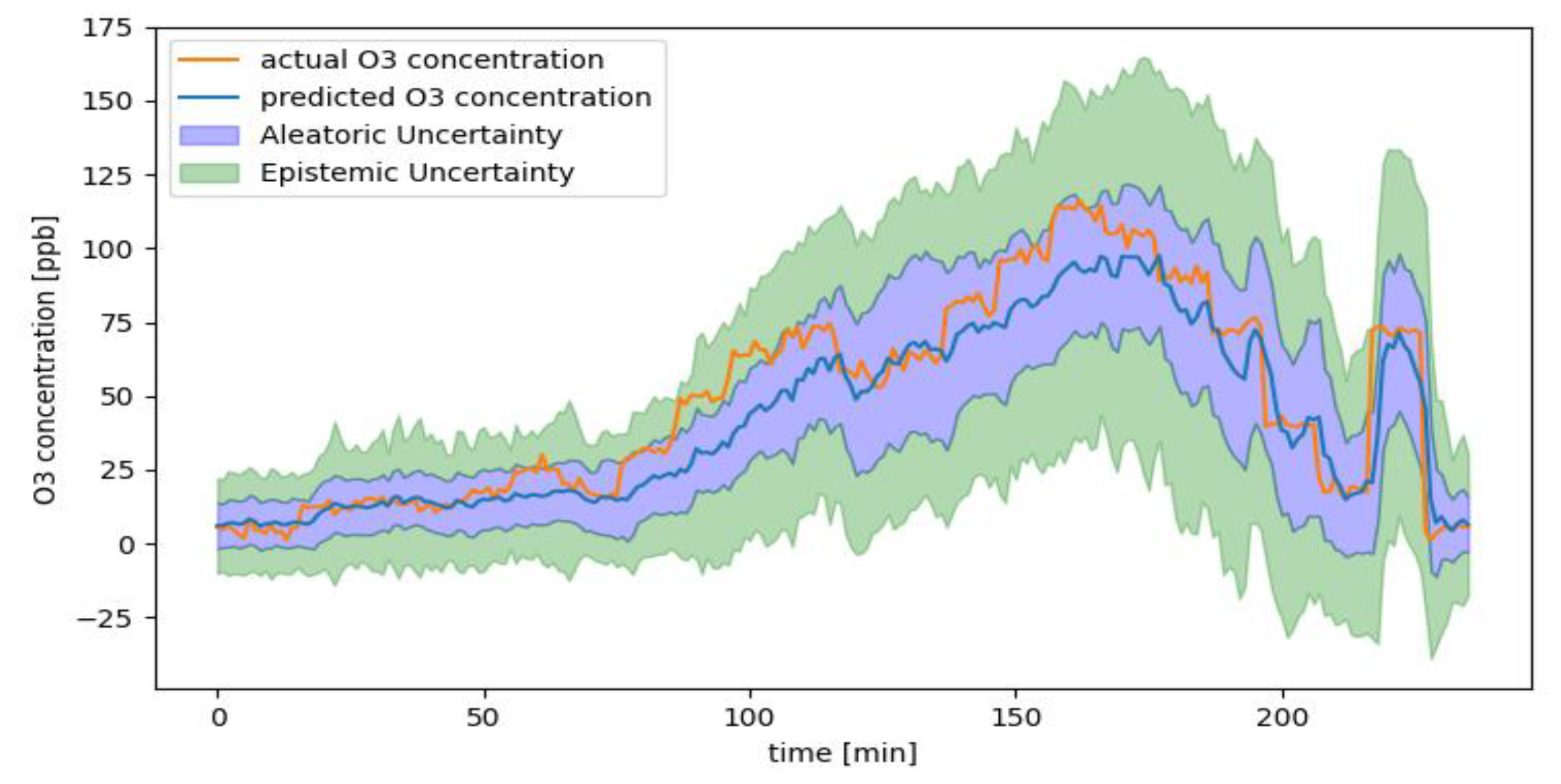
For the gas sensors under study, the data uncertainty is reflected in the different reactions of individual sensors to the same gas concentrations, i.e., sensor-to-sensor variations, and also in the same sensor reacting differently when exposed to the same gas concentrations again, which can be due to previous saturation or aging. In contrast, by quantifying model uncertainty via Bayesian deep learning, we can identify specific situations in which our model performs poorly and plan tailored experiments to generate the right training data and improve the performance of the model in these situations rather than blindly performing expensive and time-consuming measurements to generate more data overall. Figure 4 shows the model predictions for a given O3 concentration profile. Both aleatoric and epistemic uncertainty are higher for higher concentrations, which means that the sensor’s response is less consistent for higher concentrations and also that more training data for higher concentrations would be beneficial for model performance.

3. Discussion

In this work, we presented three techniques that help with understanding why and how our model generates specific concentration predictions from a low-cost gas sensor.
First, we saw how SHAP analysis helped in the decision-making process of a model based on various input features and provides useful information about the underlying sensing mechanism and technology. Furthermore, SHAP analysis aided in developing a more efficient model by identifying features that did not contribute much to the predictions, such as higher-order harmonics, and, therefore, assisted in dropping off those features from our study. When working with smart sensors, such models with fewer dimensions are especially advantageous since they require less memory and processing power, thus saving energy.
The second approach helped dive inside the model’s inner architecture. This method demonstrated that even black-box models like GRU can be quite transparent, making it still possible to trace the underlying rationale of its components.
Finally, we used approaches from Bayesian deep learning to quantify model and data uncertainty in our gas concentration predictions. This information allowed for identifying situations where more data was needed to improve the model via epistemic uncertainty as well as situations that could not be improved with more data or different model decisions and therefore need to be solved at the sensor technology level.

Author Contributions

Conceptualization, S.C., S.M. and C.C.; methodology, S.C. and S.M.; software, S.C.; validation, S.C., S.M. and C.C.; formal analysis, S.C. and S.M.; investigation, S.C. and S.M.; resources, C.C.; data curation, C.C.; writing—original draft preparation, S.C.; writing—review and editing, C.C. and S.M.; visualization, S.C. and S.M.; supervision, C.C. and S.M.; project administration, C.C. All authors have read and agreed to the published version of the manuscript.

Funding

This research received no external funding.

Institutional Review Board Statement

Not applicable.

Informed Consent Statement

Not applicable.

Data Availability Statement

Not applicable.

Conflicts of Interest

The authors declare no conflict of interest.

References

  1. Zöpfl, A.; Lemberger, M.M.; König, M.; Ruhl, G.; Matysik, F.M.; Hirsch, T. Reduced graphene oxide and graphene composite materials for improved gas sensing at low temperature. Faraday Discuss. 2014, 173, 403–414. [Google Scholar] [CrossRef] [PubMed] [Green Version]
  2. Hayasaka, T.; Lin, A.; Copa, V.C.; Lopez, L.P.; Loberternos, R.A.; Ballesteros, L.I.; Kubota, Y.; Liu, Y.; Salvador, A.A.; Lin, L. An electronic nose using a single graphene FET and machine learning for water, methanol, and ethanol. Microsyst. Nanoeng. 2020, 6, 50. [Google Scholar] [CrossRef] [PubMed]
  3. Cho, K.; Van Merriënboer, B.; Bahdanau, D.; Bengio, Y. On the properties of neural machine translation: Encoder-decoder approaches. In Proceedings of the SSST-8, Eighth Workshop on Syntax, Semantics and Structure in Statistical Translation, Doha, Qatar, 25 October 2014; pp. 103–111. [Google Scholar]
  4. Jordan, M.I.; Mitchell, T.M. Machine learning: Trends, perspectives, and prospects. Science 2015, 349, 255–260. [Google Scholar] [CrossRef] [PubMed]
  5. Goodfellow, I.; Bengio, Y.; Courville, A. Deep Learning; MIT Press: Cambridge, MA, USA, 2016. [Google Scholar]
  6. Murdoch, W.J.; Singh, C.; Kumbier, K.; Abbasi-Asl, R.; Yu, B. Definitions, methods, and applications in interpretable machine learning. Proc. Natl. Acad. Sci. USA 2019, 116, 22071–22080. [Google Scholar] [CrossRef] [PubMed] [Green Version]
  7. Doshi-Velez, F.; Kim, B. Towards a rigorous science of interpretable machine learning. arXiv 2017, arXiv:1702.08608. [Google Scholar]
  8. Lipton, Z.C. The mythos of model interpretability: In machine learning, the concept of interpretability is both important and slippery. Queue 2018, 16, 31–57. [Google Scholar] [CrossRef]
  9. Malhi, A.; Kampik, T.; Pannu, H.; Madhikermi, M.; Främling, K. Explaining machine learning-based classifications of in-vivo gastral images. In Proceedings of the 2019 Digital Image Computing: Techniques and Applications (DICTA), Perth, WA, Australia, 2–4 December 2019; pp. 1–7. [Google Scholar]
  10. Lundberg, S.M.; Lee, S.I. A unified approach to interpreting model predictions. In Proceedings of the 31st International Conference on Neural Information Processing Systems, Long Beach, CA, USA, 4–9 December 2017; pp. 4768–4777. [Google Scholar]
  11. Psychoula, I.; Gutmann, A.; Mainali, P.; Lee, S.H.; Dunphy, P.; Petitcolas, F. Explainable machine learning for fraud detection. Computer 2021, 54, 49–59. [Google Scholar] [CrossRef]
  12. Dave, D.; Naik, H.; Singhal, S.; Patel, P. Explainable ai meets healthcare: A study on heart disease dataset. arXiv 2020, arXiv:2011.03195. [Google Scholar]
  13. Karpathy, A.; Johnson, J.; Fei-Fei, L. Visualizing and understanding recurrent networks. arXiv 2015, arXiv:1506.02078. [Google Scholar]
  14. Tang, Z.; Shi, Y.; Wang, D.; Feng, Y.; Zhang, S. Memory visualization for gated recurrent neural networks in speech recognition. In Proceedings of the 2017 IEEE International Conference on Acoustics, Speech and Signal Processing (ICASSP), New Orleans, LA, USA, 5–9 March 2017; pp. 2736–2740. [Google Scholar]
  15. Kendall, A.; Gal, Y. What uncertainties do we need in bayesian deep learning for computer vision? In Proceedings of the 31st International Conference on Neural Information Processing Systems, Long Beach, CA, USA, 4–9 December 2017; pp. 5580–5590. [Google Scholar]
  16. Shapley, L. 7. A Value for n-Person Games. Contributions to the Theory of Games II (1953) 307–317. In Classics in Game Theory; Princeton University Press: Princeton, NJ, USA, 2020; pp. 69–79. [Google Scholar]
  17. Molnar, C. Interpretable Machine Learning. A Guide for Making Black Box Models Explainable. Available online: https://originalstatic.aminer.cn/misc/pdf/Molnar-interpretable-machine-learning_compressed.pdf (accessed on 1 June 2021).
  18. Vergara, A.; Martinelli, E.; Llobet, E.; D’Amico, A.; Di Natale, C. Optimized feature extraction for temperature-modulated gas sensors. J. Sens. 2009, 2009, 716316. [Google Scholar] [CrossRef] [Green Version]
  19. Tembhurne, J.V.; Diwan, T. Sentiment analysis in textual, visual and multimodal inputs using recurrent neural networks. Multimed. Tools Appl. 2021, 80, 6871–6910. [Google Scholar] [CrossRef]
  20. Gal, Y.; Ghahramani, Z. Dropout as a bayesian approximation: Representing model uncertainty in deep learning. In Proceedings of the 33rd International Conference on International Conference on Machine Learning, New York, NY, USA, 19–24 June 2016; pp. 1050–1059. [Google Scholar]
  21. Srivastava, N.; Hinton, G.; Krizhevsky, A.; Sutskever, I.; Salakhutdinov, R. Dropout: A simple way to prevent neural networks from overfitting. J. Mach. Learn. Res. 2014, 15, 1929–1958. [Google Scholar]
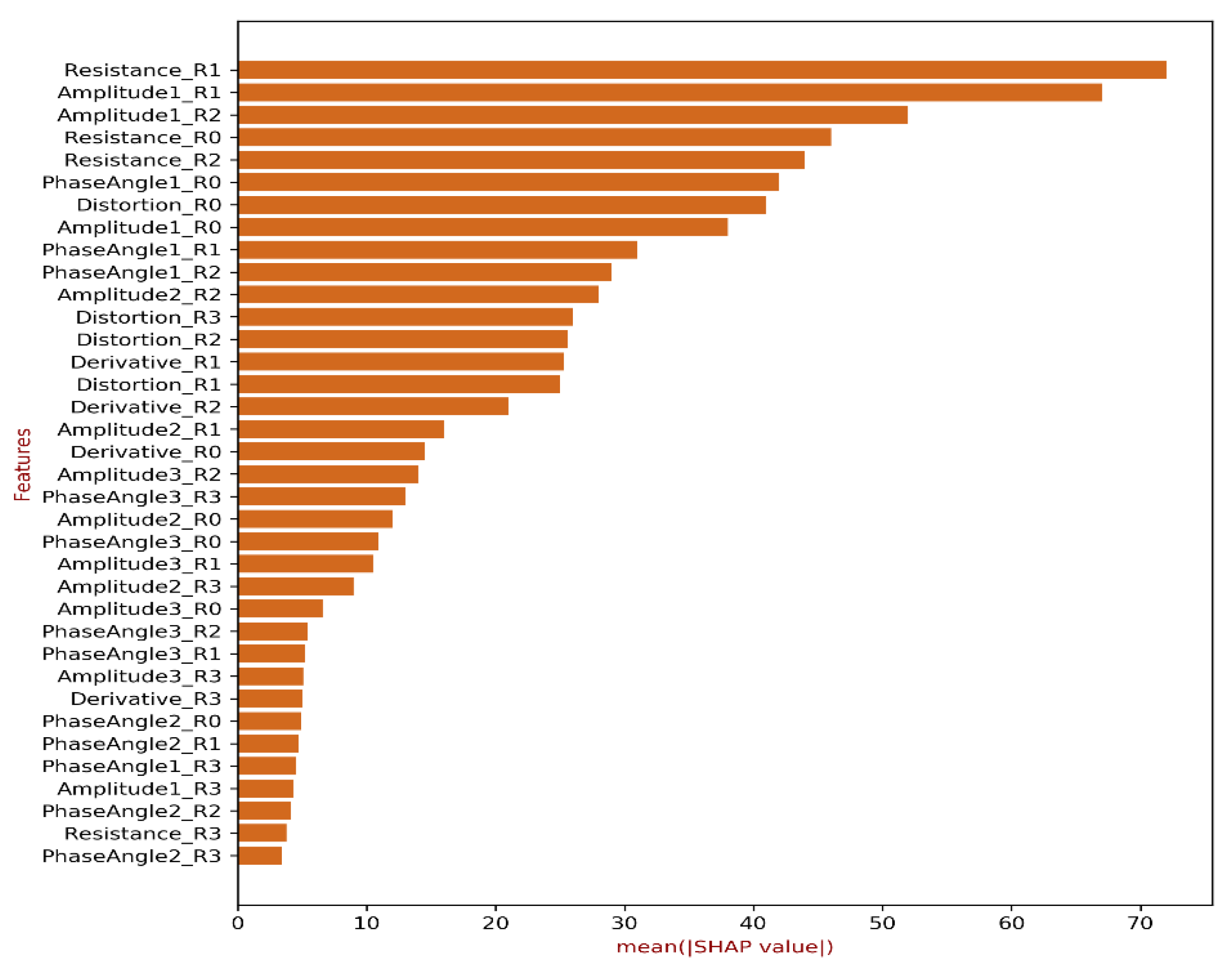
Figure 1. SHAP variable importance plot. The features include resistance, derivative, amplitude (n), phase angle (n), and distortion for each of the four sensing fields. Here, n = 1, 2, and 3, representing the 1st, 2nd, and 3rd harmonics, respectively.
Engproc 27 00061 g001
Figure 2. SHAP variable importance plot for our model with reduced feature set and improved material.
Engproc 27 00061 g002
Figure 3. Activations of units. The orange dots show positive activations and the blue dots show negative activations.
Engproc 27 00061 g003
Figure 4. Model predictions (blue) for a given O3 concentration profile (orange). Both the aleatoric and epistemic uncertainty (light blue and green, respectively) are visualized by defining a region of ±2σ for each uncertainty around the mean prediction.
Engproc 27 00061 g004
Publisher’s Note: MDPI stays neutral with regard to jurisdictional claims in published maps and institutional affiliations.