Control System Design for a Semi-Finished Product Considering Over- and Underbending ^†

Abstract

In the last decades, the application of automatic control techniques in freeform bending processes was limited to the motion control of the bending die, i.e., the workpiece itself was not considered inside the closed-loop control system. In a previous work, a simple preliminary model for the workpiece was used as a foundation for developing a closed-loop system for freeform bending that includes both the geometry and the mechanical properties of the semi-finished product. However, this approach did not consider the fact that the same geometry can be reached by either over- or underbending the tube. In this work, the previously developed system model is extended to include this physical property of the system.

1. Introduction

In freeform bending, the application of closed-loop control systems (to the author’s best knowledge) has been limited to the motion control of the tool head itself, where the motion trajectory is fed into the Programmable Logical Controller (PLC) of the CNC Machine in the form of a G-Code. The internal controller of the actuator then guarantees that the given trajectory is followed up. However, this does not guarantee that the desired workpiece characteristics are maintained since they remain unconsidered outside the closed-loop control system. In [1], a preliminary approach was considered, in order to include the bent curvature, as well as the residual stresses inside the tube, in the closed-loop control system. In this approach, only tangential bending was considered. However, in [2], it was proven that the same bending curvature could still be reached using a wide range of bending head movement combinations y and α see Figure 1. In this work, the previously developed model is to be modified to include the extra bending possibilities due to over- and underbending.

1.1. Freeform Bending State of the Art

Freeform bending with a movable die is a novel forming technology that allows for the bending of the workpiece into complex geometries without the need to change the bending tool itself. The mechanical construction and the main functionality of each component have been thoroughly discussed previously in [1,2].

In [1], the foundation for a preliminary control-loop structure of a freeform bending machine was laid. Thereby a physical, rheological model based on the Masing model with a Saint Venant Element was utilized for the derivation of a mathematical formulation for the elastic-plastic deformation process. For the modeling of the residual stresses, the hydrostatic pressure was chosen as an indicator. An empirical equation was identified that related the temperature and curvature with the hydrostatic pressure. However, in [2], it was shown that residual stresses were not only affected by heating but also by applying different combinations of displacements y and rotations α of the bending die. Two different bending techniques were addressed, which were: tangential bending and non-tangential bending. Tangential bending can be defined as the bending process when the bending die is oriented based on the kinematic construction of the machine itself (which is the case in [1]). Non-tangential bending, however, is when the bending die of the tube is slightly bent over the tangential bending (Overbending) or slightly bent under the tangential bending (Underbending) (as shown in Figure 1). By introducing the concept of non-tangential bending, it is possible to get the same bending geometry using different combinations of y and α. It was also shown that different stress states for the same bent geometries could be reached by using over- and underbending, thus decoupling the bending geometry from the respective mechanical properties. In order to be able to consider the residual stresses inside the workpiece, a foundation for a soft sensor based on an extended Kalman filter (EKF) was laid in [3,4].

1.2. Goals and Assumptions

In the previous work [1] the main goal was to propose a control structure for the freeform bending machine that took both the geometry (curvature) as well as the residual stresses into consideration inside the closed-loop control system. In this contribution, the previously designed model was modified and extended to include non-tangential bending (over- and underbending). The goal thereby was to find a mathematical formulation that related different combinations of y and α with their respective curvature and residual stresses.

The same assumptions that were made in [1] were still valid in this work here; the 6 degrees of freedom (DOF) were reduced to 3 DOF for the sake of simplicity (2 DOF for the bending die and 1 DOF for the tube feeder). Moreover, it was assumed that the temperature of the workpiece remained constant during the bending process; the heating unit that was considered in the previous work [1] was eliminated in this work, and the change in residual stresses was only considered due to the followed bending strategy. To be noted here is that all results were based on finite element simulations depicted in [2].

2. Materials and Methods

In the previous work [1], a rheological mathematical model was sought in order to mathematically describe the relationship between the resulting end curvature ${\kappa }_{act}$ with the respective bending die orientation $\alpha$ (see Figure 1).

$${\phi }_p=\frac{k_e}{k_e+k_p}\alpha ,\mathrm{with}$$

(1)

$$\alpha =d_a\ast {\kappa }_B,{\phi }_p=d_a\ast {\kappa }_{act},\mathrm{hence}$$

(2)

$${\kappa }_{\mathrm{act}}=\frac{K_e}{K_e+K_p}\ast {\kappa }_{\mathrm{des}},$$

(3)

${\kappa }_{act}=1/R_{act}$ and ${\kappa }_{des}=1/R_{des}$ distance between the tube guide and the bending die, α is the orientation of the bending die, φp is the plastically deformed bent angle of the tube after unloading considering the spring-back effect, Ke, Kp are the stiffnesses of the material in the elastic and plastic region of deformation respectively. The vertical displacement of the bending die y can be calculated geometrically based on the machine construction,

$$y=\frac{1-\cos \left(\alpha \right)}{{\kappa }_{des}}.$$

(4)

A thorough discussion of the derivation of the previous equations has already been done in a previous work [1]. The bending process carried out based on these equations is called tangential bending. In this work, however, a mathematical relationship between the resulting curvature and residual stresses altogether with the non-tangential bending was to be investigated. This was done based on simulation results out of a Finite Element Modell (FEM). According to [2,4], this model has proven to be seemingly accurate in a reliable way and therefore has been further used for the derivation of the mathematical formulations for the non-tangential bending.

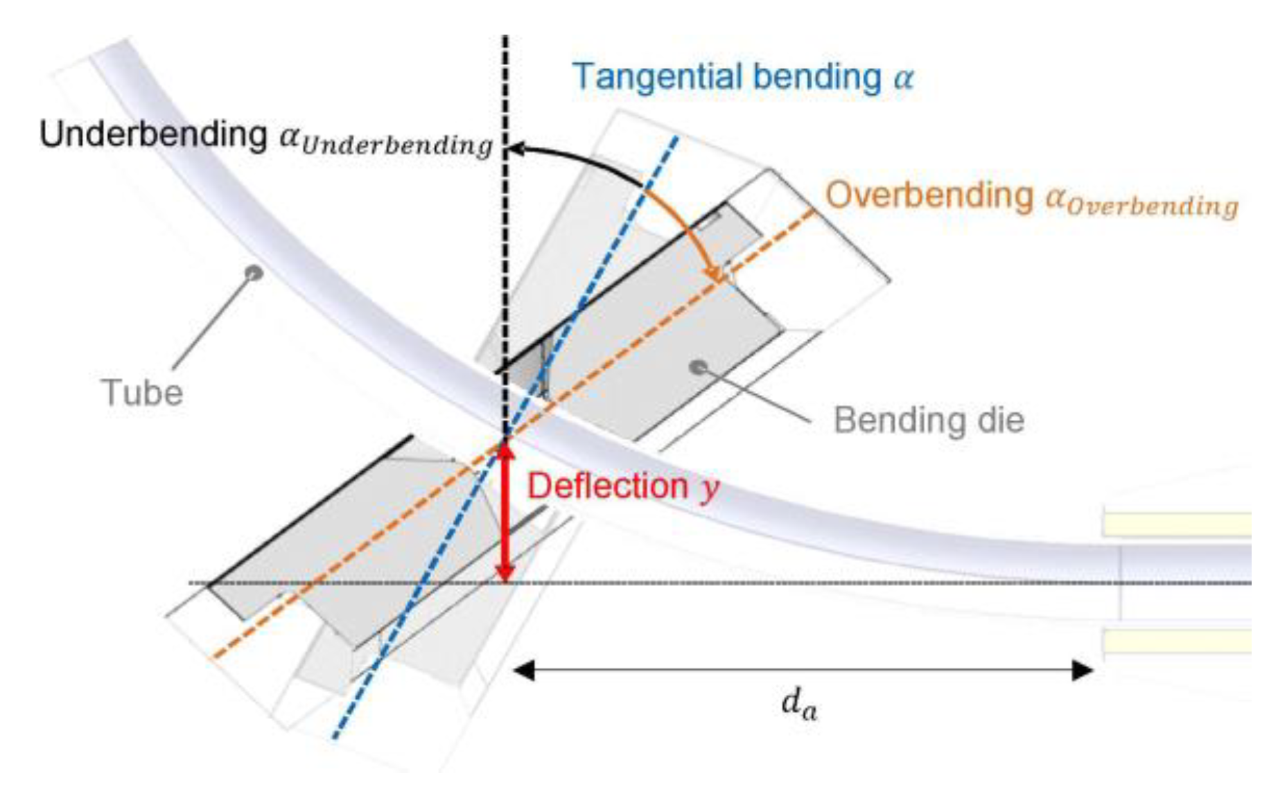
2.1. Mathematical Model for Curvature in Non-Tangential Bending

In this section, the mathematical relationship between the inputs α and y and the resulting curvature was to be investigated. To that end, different data relating the output curvature altogether with its respective bending die dislocations (y and α) were gathered (based on the simulation results of FEM). In

Table 1. Different combinations between y and α.

y (mm)									α (°)
5	0	1	2	3	4	5	6	7	8	9	10	11	12	13	14	15	16
6	2	3	4	5	6	7	8	9	10	11	12	13	14	15	16	17	18
7	3	4	5	6	7	8	9	10	11	12	13	14	15	16	17	18	19
8	5	6	7	8	9	10	11	12	13	14	15	16	17	18	19	20	21
9	6	7	8	9	10	11	12	13	14	15	16	17	18	19	20	21	22
10	7	8	9	10	11	12	13	14	15	16	17	18	19	20	21	22	23
11	9	10	11	12	13	14	15	16	17	18	19	20	21	22	23	24	25
12	10	11	12	13	14	15	16	17	18	19	20	21	22	23	24	25	26
13	12	13	14	15	16	17	18	19	20	21	22	23	24	25	26	27	28
14	13	14	15	16	17	18	19	20	21	22	23	24	25	26	27	28	29
15	14	15	16	17	18	19	20	21	22	23	24	25	26	27	28	29	30

, the different combinations of y and α are tabulated.

Figure 2 displays the resulting curvature of different combinations for y = 15 mm with varying α, as seen in the last row of Table 1. The solid and dashed red lines represent the motion trajectory of the bending die about the x-axis α and along the y-axis, respectively, whereas the solid blue line represents the resulting curvature κ (in mm⁻¹). It can be inferred that the curvature of the tube undergoes some sort of overshooting upon starting or ending the bending process. One explanation for that behavior is that the circularity of the tube profile can no longer be perfectly maintained in these transition regions, i.e., the tube profile gets distorted and takes, to some extent, an elliptical shape. This profile distortion results in some ripples on the surface of the tube during these transition regions. However, in this work, this dynamic-like behavior is neglected, and only the static behavior was taken into consideration. Therefore, the average of the resulting curvature along the tube is taken further into consideration. The same applies to the other different combinations of y and α. Figure 3 shows a 3D representation of the average curvature against the y and α combinations depicted in Table 1.

Now that the data was collected and tabulated, the mathematical relationship would be investigated. For that, five different approaches were considered, and the respective deviation norm was calculated for each. However, for the sake of briefness, only two approaches are represented here. The first approach (Equation (5)) was motivated by the kinematic model that had been previously derived in [1]. In Equation (6), a quadratic approach motivated out of the Taylor series was tested:

$$\kappa =\frac{a+bcos\left(\alpha \right)}{y}$$

(5)

$$\kappa =ay+b\alpha +c{y}^2+d{\alpha }^2$$

(6)

For each approach, the respective a, b, c, and d parameters were identified. Here the least square method was deployed. Taking the second approach, Equation (6), as an example, the equation can be rewritten in a matrix form as follows:

$$\mathit{\kappa }=\left[\begin{array}{cccc}\mathit{y}& \mathit{\alpha }& {\mathit{y}}^{\mathbf{2}}& {\mathit{\alpha }}^{\mathbf{2}}\end{array}\right]{\left[\begin{array}{cccc}a& b& c& d\end{array}\right]}^T =\mathit{A}\mathit{P}$$

(7)

A in this case, is a matrix composed of the vectors y, α, y², α² that maps between the parameter vector P with the output vector κ. The vectors y, α, and κ were measured based on the simulation results of the FEM. Since matrix A was a non-square matrix, the pseudo inverse was calculated in order to identify the parameter vector P for each approach (see Equation (8)). Figure 4 shows the identified parameters as well as a comparison between the first approach and the quadratic approach.

$$\mathit{P}={\left({\mathit{A}}^{\mathit{T}}\mathit{A}\right)}^{\mathbf{-}\mathbf{1}}{\mathit{A}}^{\mathit{T}}\mathit{\kappa }={\mathit{A}}^{†}\mathit{\kappa }$$

(8)

It can be inferred that the approach motivated by the kinematic model had the highest deviation norm among the other approaches (1.5 × 10⁻³). Using the quadratic approach, very good compliance between the FEM results and the results of the static model was reached. In order to check whether adding more terms significantly improved the deviation norm, a fifth mixed term was introduced to the quadratic approach. However, this extra term did not significantly improve the error. Therefore, the quadratic approach, Equation (6), was accepted as a mathematical representation of the curvature in conjunction with non-tangential bending.

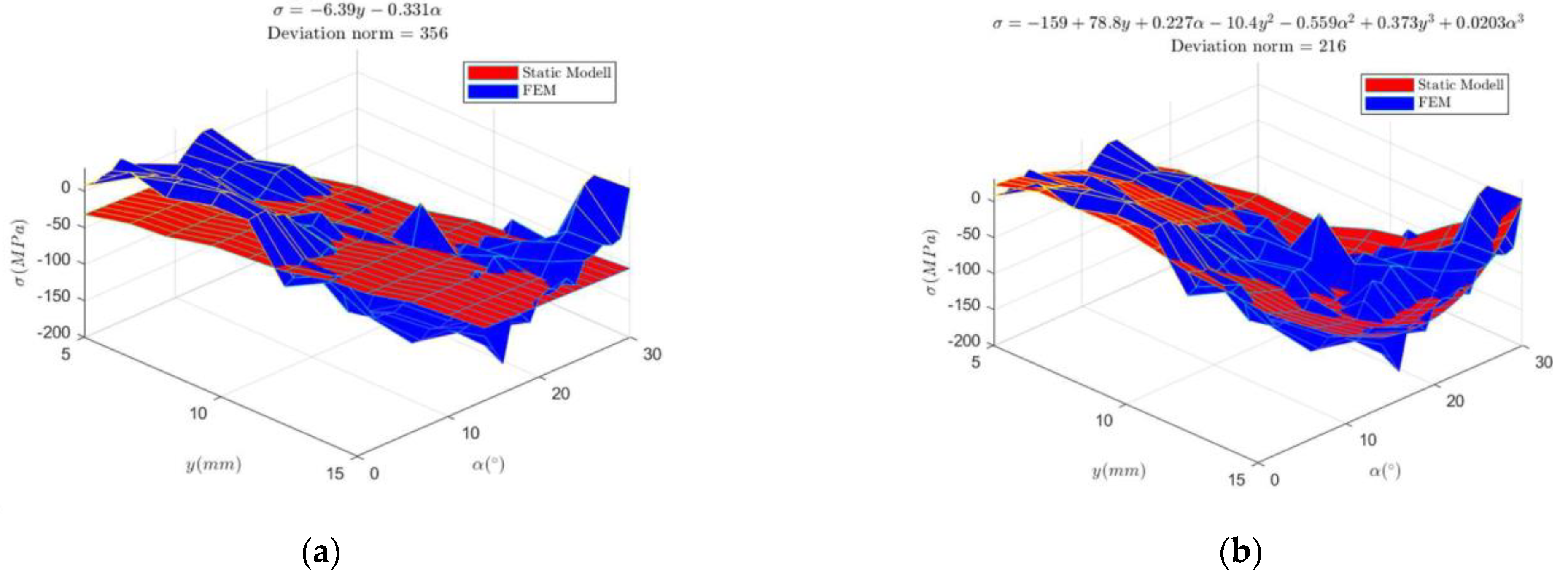
2.2. Mathematical Model for Residual Stresses in Non-Tangential Bending

Here, the same y and α combinations depicted in Table 1 were utilized. The data of the residual stresses were also collected from the same FEM. Figure 5 shows the simulation results of the last row of Table 1. The residual stresses represented here are those on the surface of the inner curve of the bent tube, i.e., the surface that was undergoing compression. In addition, here, the average value of the curvature κ for each y and α combination was taken since the static behavior of the system was the main focus of this work.

For system identification, five different approaches were also tested: a linear approach, a quadratic approach, a cubic approach, and a quartic approach. The parameters of each approach were identified using the same least square method that was previously discussed in the last subsection. For the sake of briefness, only two approaches were represented and compared to their respective FEM simulations (see Figure 6). It can be inferred that the cubic approach has a lower deviation norm compared to the linear approach.

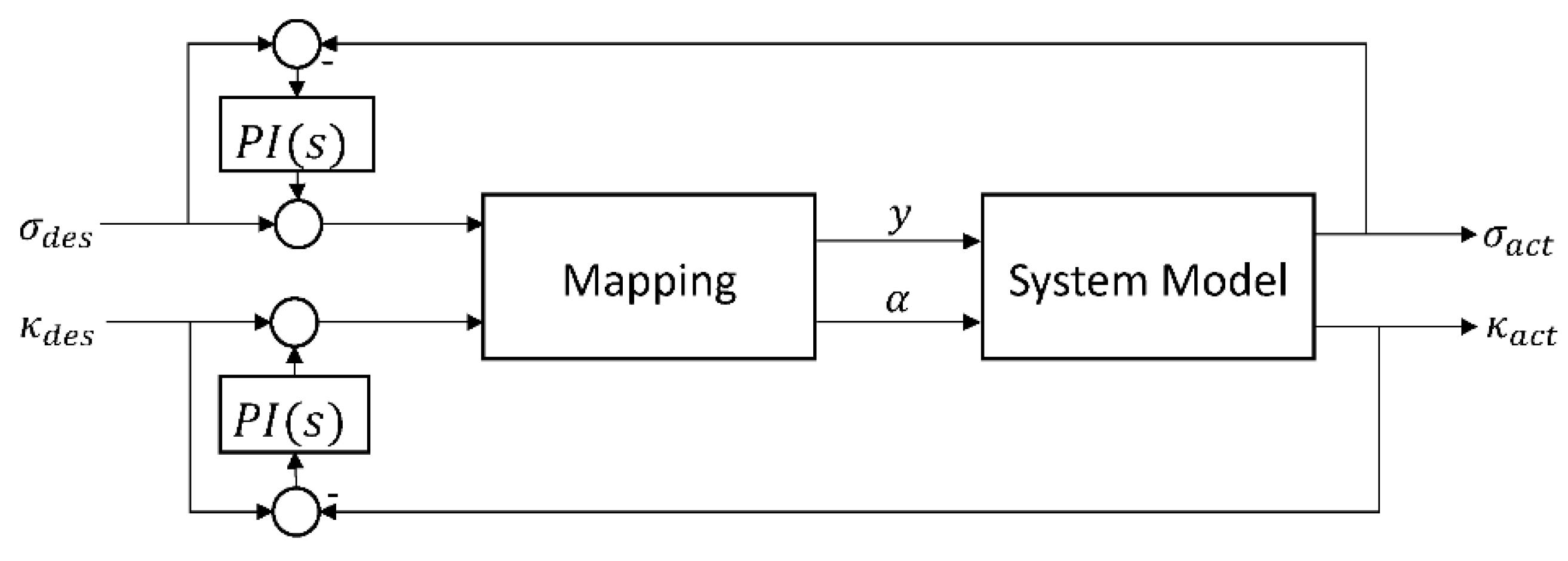
3. Developing a Closed-Loop Control System

In the preceding section, a mathematical model was developed for each curvature and residual stress. For the curvature, the quadratic approach was accepted:

$$\kappa =2.504\times {10}^{-4}y+6.517\times {10}^{-5}\alpha -3.888\times y^2-8.516\times {10}^{-7}{\alpha }^2,$$

(9)

The physical units are omitted for the sake of visual clarity. For the residual stresses, the cubic approach showed the least deviation with the minimum number of terms. How- ever, to simplify the equation inversion for the development of the mapping function, the linear approach was accepted as a simplified mathematical representation.

$$\sigma =-6.39y-0.331\alpha$$

(10)

Figure 7 shows a newly proposed closed-loop control system structure that takes the effect of non-tangential bending into account. Here, the actual residual stresses σ_act, as well as the actual curvature κ_act, are to be compared with their respective desired residual stresses σ_des and curvature κ_des. The deviation is then introduced to a PI-Controller that, in turn, produces a correction signal to be augmented on the feedforward signal. The result is then introduced to a mapping block, which, in turn, translates these signals into the respective bending die translation and orientation.

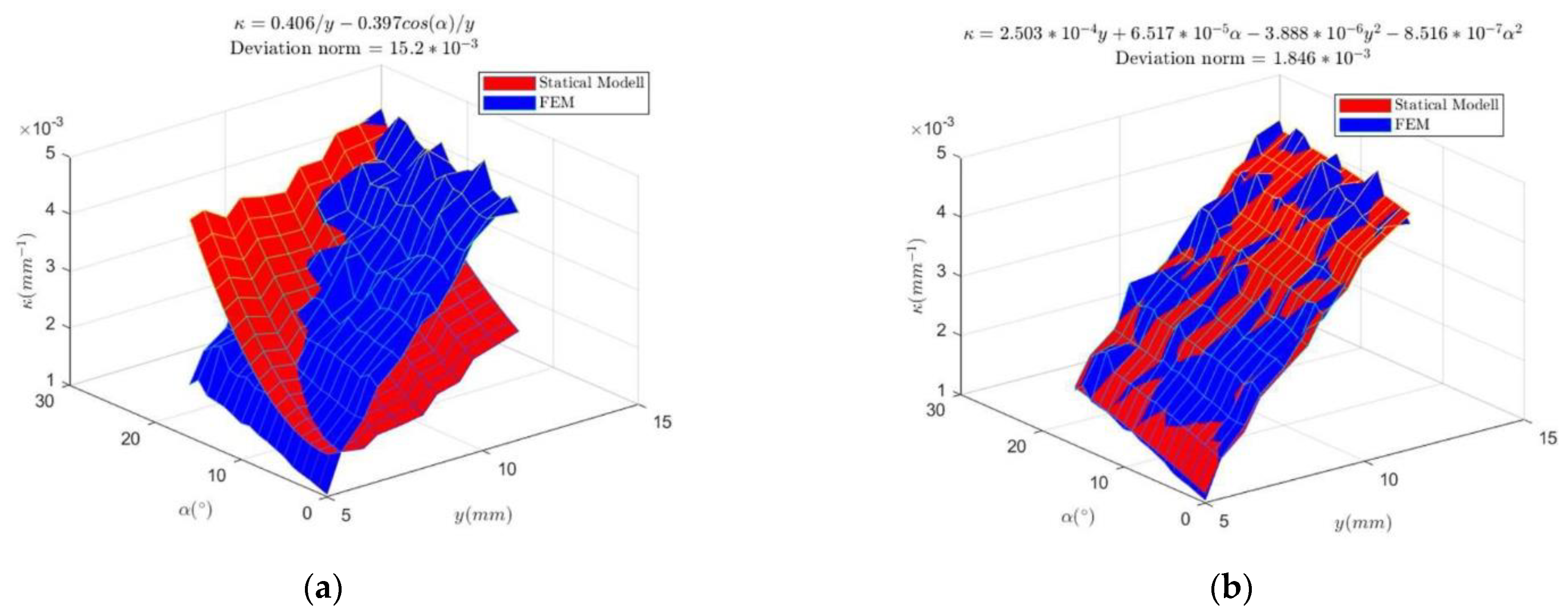
3.1. Deriving the Mathematical Equations for the Mapping Block

The mathematical equations for the mapping block can be derived based on Equations (9) and (10). For this reason, the linear approach for the residual stresses has been taken further since it can be simply inverted. Equation (10) can be rewritten in terms of α as follows:

$$\alpha =-19.305y-3.021\sigma$$

(11)

by substituting in Equation (9):

$$\begin{array}{c}\kappa =2.503\times {10}^{-4}y+6.517\times {10}^{-5}\left(-19.305y-3.021\sigma \right)-3.888\times {10}^{-6}{y}^2-\\ 8.516\times {10}^{-7}{\left(-19.305y-3.021\sigma \right)}^2,\end{array}$$

which can be further simplified to:

$$y^2+\left(0.31\sigma +3.15\right)y+0.02{\sigma }^2+0.61\sigma +3116.24\kappa =0$$

(12)

This equation can now be solved by using the quadratic equation $y_{1,2}=-p/2\pm \sqrt{p^2/2-q}$ where $p=0.31\sigma +3.15$ and $q=0.02{\sigma }^2+0.61\sigma +3116.24\kappa$. By substituting for y_1,2 in Equation (11), the corresponding bending orientation α can be calculated. In order to determine which value for y and α should be accepted, the boundary conditions should be taken into consideration. Hereby the case where y = 0 and α = 0 is considered. In this case, the curvature and residual stresses are expected to be zero for each. This is also verified using Equations (9) and (10). In order to check whether this condition is not violated, we substitute with σ = 0 MPa and κ = 0 mm⁻¹ in the parameters of the quadratic equation (p and q). In that case, the parameters will be $p=3.15$ and $q=0$; i.e.,$y_{1,2}=-\left(3.15/2\right)\pm \sqrt{{\left(3.15/2\right)}^2-0}$. This shows that the boundary condition $\left(y=0 \forall \kappa =0 {\mathrm{mm}}^{-1}, \sigma =0 \mathrm{MPa}\right)$ can only be achieved when:

$$y=y_1=-\frac{p}{2}+\sqrt{\frac{p^2}{4}-q}$$

(13)

By substituting Equation (13) in Equation (11), the bending die orientation α will be:

$$\alpha =-19.305y_1-3.021\sigma$$

(14)

It can easily be checked that for y₁ = 0 mm and σ = 0 MPa, the bending die orientation α is also 0°. Equations (13) and (14) are implemented inside the mapping block depicted in Figure 7. In the following section, the model earlier introduced is simulated.

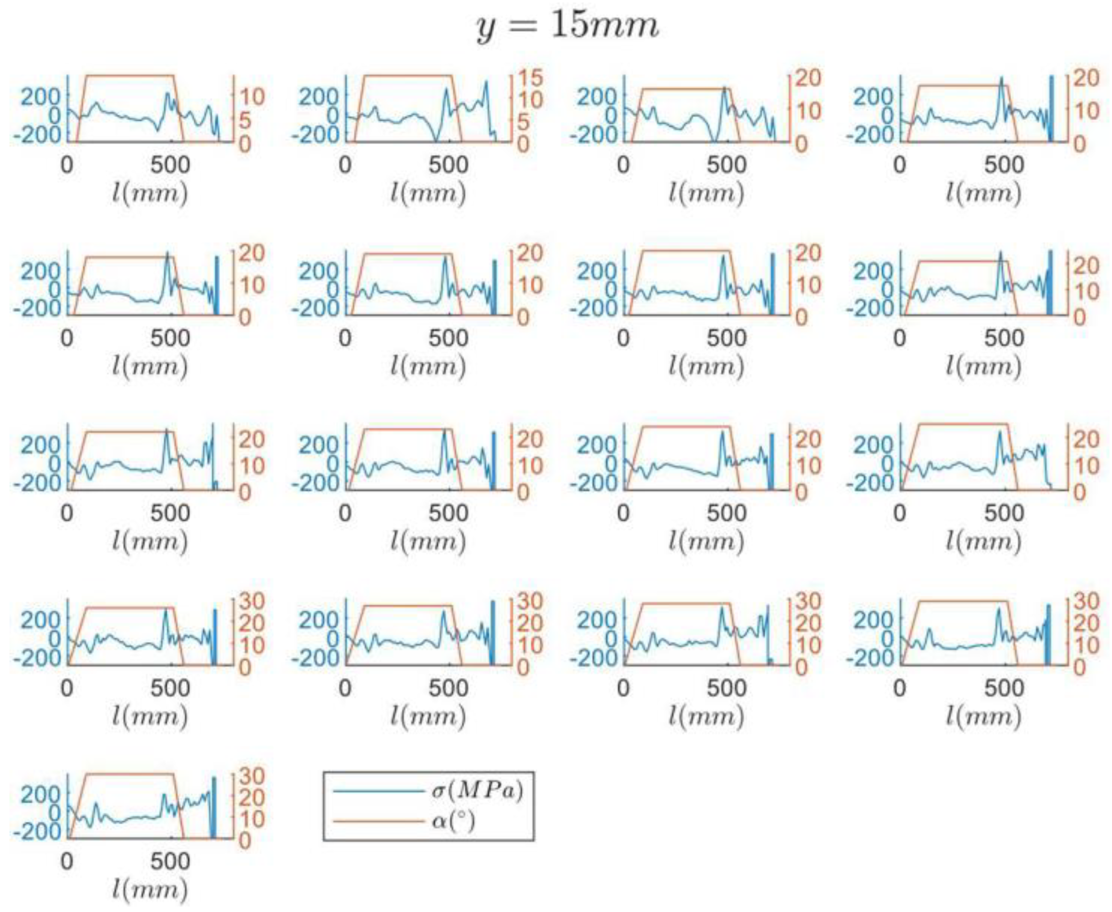
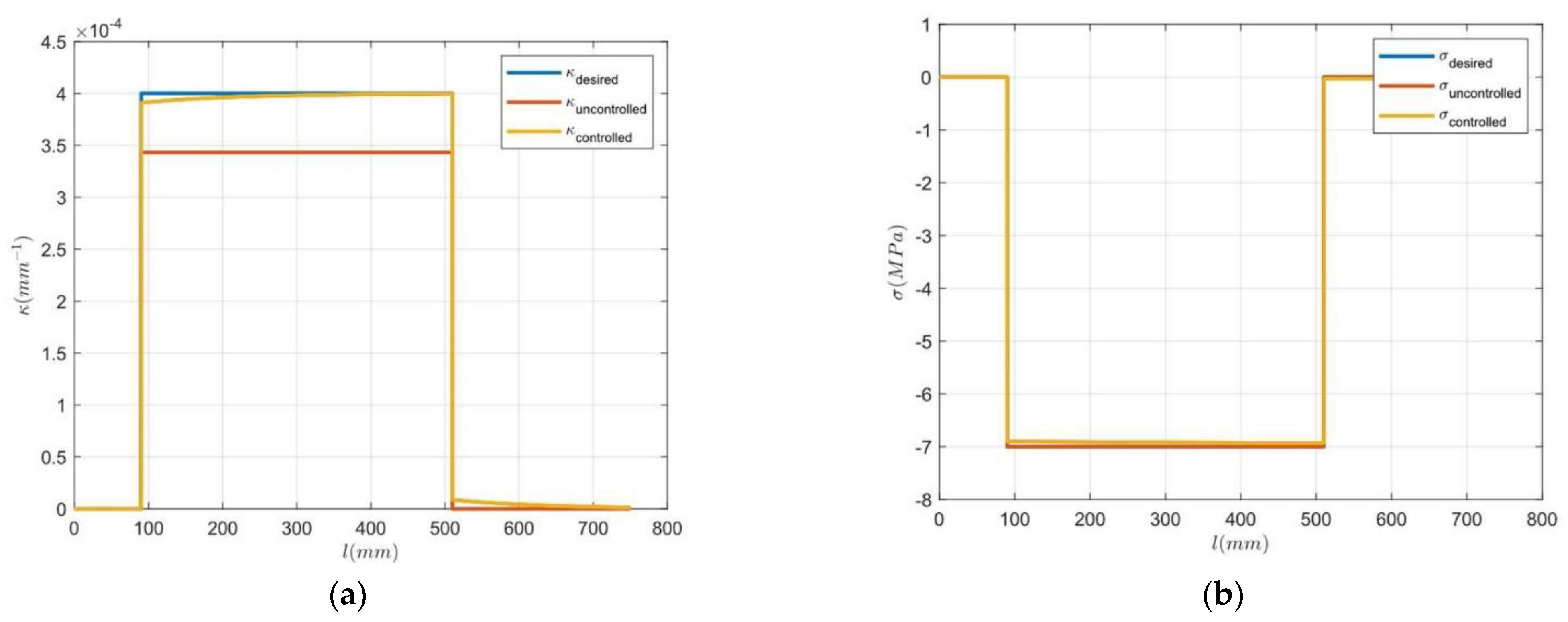
3.2. Simulation Results

The previous control scheme depicted in Figure 7 was implemented and simulated using the MATLAB-Simulink software package. Figure 8 shows the simulation results for the curvature and residual stresses, respectively. From there, it can be inferred that the trajectory of the actual residual stresses without a controller coincides with the respective desired residual stress. In contrast, the actual curvature deviates to some extent from the desired curvature. This can be justified by the fact that the identified models are full of uncertainties. For example, a linear model for the residual stresses was chosen to simplify the inversion of the function for the mapping block. However, the introduction of a PI controller significantly improved the coincidence of the actual curvature trajectory with its respective desired trajectory (see Figure 8a). This improvement came at the cost of the residual stresses, i.e., the actual trajectory of the residual stresses has to some extent, lost its coincidence with its respective desired trajectory (Figure 8b). This can be again justified by the fact that the chosen models are full of uncertainties to be dealt with in the upcoming works.

4. Conclusions and Discussion

In this work, a mathematical representation of the non-tangential bending was proposed and simulated via MATLAB-Simulink. The simulation results showed that it was possible to control the residual stresses decoupled from the respective curvature. The model of the residual stresses was greatly simplified in order to facilitate the design of the mapping function that converted the κ and σ signals into respective bending die movements (y and α). This simplification came to be expected with some measure of sacrificing the accuracy of the coincidence of the desired and actual curvature trajectories. The introduction of a PI controller, however, could significantly improve the quality of the desired actual trajectory follow-up. In upcoming works, this problem can be solved by training a neural network or a Bayesian Gaussian process [5] that is able to include all the non-linearities out of the measurements and develop a more accurate model for the curvature and residual stresses, respectively, as well as a more accurate mathematical function for the mapping block.

It must be noted that this work focuses only on the static behavior of the workpiece during freeform bending; the dynamic-like behavior depicted in Figure 2 is not considered. This behavior should be a concern for upcoming work as it constitutes an important step for deriving a formula for predicting the error propagation along the tube and, accordingly, designing a predictive controller that is able to minimize this error in an optimized way. In [6], an approach for the trajectory prediction of the freeform bending process based on an extended Kalman filter was introduced. Moreover, a heating system is planned to be embedded inside the bending machine for the further adjustment of the residual stresses inside the tube [7].

References

1. Ismail, A.; Maier, D.; Stebner, S.; Volk, W.; Münstermann, S.; Lohmann, B. A Structure for the Control of Geometry and Properties of a Freeform Bending Process. IFAC-PapersOnLine 2021, 54, 115–120. [Google Scholar] [CrossRef]
2. Maier, D.; Stebner, S.; Ismail, A.; Dölz, M.; Lohmann, B.; Münstermann, S.; Volk, W. The influence of freeform bending process parameters on residual stresses for steel tubes. Adv. Ind. Manuf. Eng. 2021, 2, 100047. [Google Scholar] [CrossRef]
3. Stebner, S.C.; Maier, D.; Ismail, A.; Balyan, S.; Dölz, M.; Lohmann, B.; Volk, W.; Münstermann, S. A System Identification and Implementation of a Soft Sensor for Freeform Bending. Materials 2021, 14, 4549. [Google Scholar] [CrossRef] [PubMed]
4. Stebner, S.C.; Maier, D.; Ismail, A.; Dölz, M.; Lohman, B.; Volk, W.; Münstermann, S. Extension of a Simulation Model of the Freeform Bending Process as Part of a Soft Sensor for a Property Control. In Key Engineering Materials; Trans Tech Publications Ltd.: Bäch, Switzerland, 2022; Volume 926, pp. 2137–2145. [Google Scholar] [CrossRef]
5. Rasmussen, C.E.; Williams, C.K.I. Gaussian Processes for Machine Learning, 3rd ed.; Adaptive Computation and Machine Learning series; MIT Press: Cambridge, MA, USA, 2008. [Google Scholar]
6. Wu, J.; Liang, B.; Yang, J. Trajectory prediction of three-dimensional forming tube based on Kalman filter. Int. J. Adv. Manuf. Technol. 2022, 121, 5235–5254. [Google Scholar] [CrossRef]
7. Maier, D.; Kerpen, C.; Werner, M.K.; Scandola, L.; Lechner, P.; Stebner, S.C.; Ismail, A.; Lohmann, B.; Münstermann, S.; Volk, W. Development of a partial heating system for freeform bending with movable die. In Hot Sheet Metal Forming of High-Performance Steel, Proceedings of the 8th International Conference, Barcelona, Spain, 20–22 April 2022; Oldenburg, M., Hardell, J., Casellas, D., Eds.; Wissenschaftliche Scripten: Auerbach/Vogtland, Germany, 2022; pp. 767–774. [Google Scholar]
Figure 1. Tangential bending, Over- and Underbending based on foundations of [2].
Engproc 26 00016 g001
Figure 2. Resulting curvature κ out of the combinations depicted in the last row of Table 1.
Engproc 26 00016 g002
Figure 3. Average curvature against different combinations of α and y.
Engproc 26 00016 g003
Figure 4. (a) First approach motivated out of the kinematic model in Equation (5), (b) Quadratic approach, Equation (6).
Engproc 26 00016 g004
Figure 5. Resulting residual stresses σ out of the combinations depicted in the last row of Table 1.
Engproc 26 00016 g005
Figure 6. (a) Linear approach and (b) cubic approach for the residual stresses.
Engproc 26 00016 g006
Figure 7. Closed-loop control system structure considering non-tangential bending.
Engproc 26 00016 g007
Figure 8. (a) Trajectories for desired curvature (in blue) actual curvature without controller (in red) and with a PI-controller (in yellow). (b) Trajectories for desired residual stresses coinciding with the actual residual stresses without controller (in red). Actual residual stresses with a PI-controller (in yellow).
Engproc 26 00016 g008