
Comparative Analysis of Residential Load Forecasting with Different Levels of Aggregation †


Abstract
:1. Introduction
2. Literature Review
3. Demand Forecasting with RNN
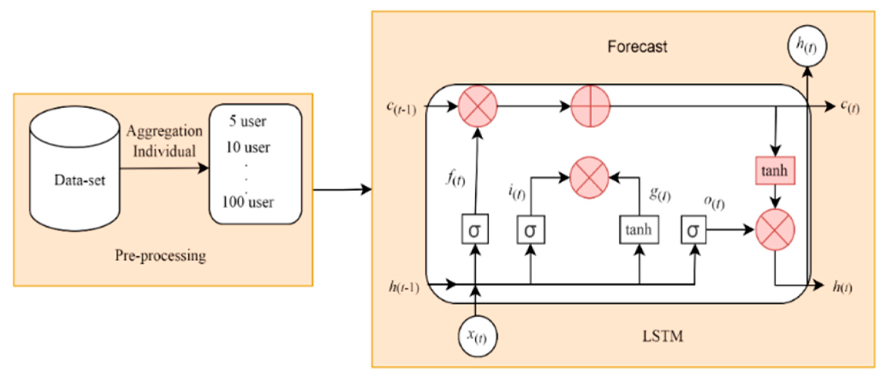
Long Short-Term Memory
4. Methodology for Comparison and Case Study
5. Results
6. Conclusions
Author Contributions
Funding
Institutional Review Board Statement
Informed Consent Statement
Data Availability Statement
Acknowledgments
Conflicts of Interest
References
- Deng, Z.; Wang, B.; Xu, Y.; Xu, T.; Liu, C.; Zhu, Z. Multi-scale convolutional neural network with time-cognition for multi-step short-Term load forecasting. IEEE Access 2019, 7, 88058–88071. [Google Scholar] [CrossRef]
- Kong, W.; Dong, Z.Y.; Hill, D.J.; Luo, F.; Xu, Y. Short-term residential load forecasting based on resident behaviour learning. IEEE Trans. Power Syst. 2018, 33, 2017–2018. [Google Scholar] [CrossRef]
- Kelly, J.; Knottenbelt, W. The UK-DALE dataset, domestic appliance-level electricity demand and whole-house demand from five UK homes. Sci. Data 2015, 2, 1–14. [Google Scholar] [CrossRef] [PubMed] [Green Version]
- Sevlian, R.; Rajagopal, R. Short Term Electricity Load Forecasting on Varying Levels of Aggregation. 2017, 1–19. Available online: http://arxiv.org/abs/1404.0058 (accessed on 17 June 2022).
- Elvers, A.; Vos, M.; Albayrak, S. Short-term probabilistic load forecasting at low aggregation levels using convolutional neural networks. In Proceedings of the 2019 IEEE Milan PowerTech, Milan, Italy, 23–27 June 2019. [Google Scholar] [CrossRef]
- Kong, W.; Dong, Z.Y.; Jia, Y.; Hill, D.J.; Xu, Y.; Zhang, Y. Short-Term Residential Load Forecasting Based on LSTM Recurrent Neural Network. IEEE Trans. Smart Grid 2019, 10, 841–851. [Google Scholar] [CrossRef]
- Gholizadeh, N.; Musilek, P. Federated learning with hyperparameter-based clustering for electrical load forecasting. Internet Things 2022, 17, 100470. [Google Scholar] [CrossRef]
- Kong, W.; Dong, Z.Y.; Luo, F.; Meng, K.; Zhang, W.; Wang, F.; Zhao, X. Effect of automatic hyperparameter tuning for residential load forecasting via deep learning. In Proceedings of the 2017 Australasian Universities Power Engineering Conference (AUPEC), Melbourne, VIC, Australia, 19–22 November 2017. [Google Scholar] [CrossRef]
- Amarasinghe, K.; Marino, D.L.; Manic, M. Deep neural networks for energy load forecasting. IEEE Int. Symp. Ind. Electron. 2017, 1483–1488. [Google Scholar] [CrossRef]
- Al Mamun, A.; Hoq, M.; Hossain, E.; Bayindir, R. A hybrid deep learning model with evolutionary algorithm for short-term load forecasting. In Proceedings of the 2019 8th International Conference on Renewable Energy Research and Applications (ICRERA), Brasov, Romania, 3–6 November 2019; pp. 886–891. [Google Scholar] [CrossRef]
- Marino, D.L.; Amarasinghe, K.; Manic, M. Building energy load forecasting using Deep Neural Networks. In Proceedings of the IECON 2016-42nd Annual Conference of the IEEE Industrial Electronics Society, Florence, Italy, 23–26 October 2016; pp. 7046–7051. [Google Scholar] [CrossRef] [Green Version]
- Somu, N.; MR, G.R.; Ramamritham, K. A hybrid model for building energy consumption forecasting using long short term memory networks. Appl. Energy 2020, 261, 114131. [Google Scholar] [CrossRef]
- Jiao, R.; Zhang, T.; Jiang, Y.; He, H. Short-term non-residential load forecasting based on multiple sequences LSTM recurrent neural network. IEEE Access 2018, 6, 59438–59448. [Google Scholar] [CrossRef]
- Hossen, T.; Nair, A.S.; Chinnathambi, R.A.; Ranganathan, P. Residential Load Forecasting Using Deep Neural Networks (DNN). In Proceedings of the 2018 North American Power Symposium (NAPS), Fargo, ND, USA, 9–11 September 2018; pp. 1–5. [Google Scholar] [CrossRef]
- Jiang, Z.; Lin, R.; Yang, F. A hybrid machine learning model for electricity consumer categorization using smart meter data. Energies 2018, 11, 2235. [Google Scholar] [CrossRef] [Green Version]
- Viegas, J.L.; Vieira, S.M.; Sousa, J.M.C. Fuzzy clustering and prediction of electricity demand based on household characteristics. In Proceedings of the 2015 Conference of the International Fuzzy Systems Association and the European Society for Fuzzy Logic and Technology, Asturias, Spain, 30 June–3 July 2015. [Google Scholar] [CrossRef] [Green Version]
- Rahman, H.; Selvarasan, I.; Jahitha Begum, A. Short-term forecasting of total energy consumption for India-a black box based approach. Energies 2018, 11, 3442. [Google Scholar] [CrossRef] [Green Version]
- Estebsari, A.; Rajabi, R. Single residential load forecasting using deep learning and image encoding techniques. Electronics 2020, 9, 68. [Google Scholar] [CrossRef] [Green Version]
- Hsiao, Y.H. Household electricity demand forecast based on context information and user daily schedule analysis from meter data. IEEE Trans. Ind. Inform. 2015, 11, 33–43. [Google Scholar] [CrossRef]
- Yan, X.; Abbes, D.; Francois, B. Uncertainty analysis for day ahead power reserve quantification in an urban microgrid including PV generators. Renew. Energy 2017, 106, 288–297. [Google Scholar] [CrossRef]
- Beccali, M.; Cellura, M.; Lo Brano, V.; Marvuglia, A. Short-term prediction of household electricity consumption: Assessing weather sensitivity in a Mediterranean area. Renew. Sustain. Energy Rev. 2008, 12, 2040–2065. [Google Scholar] [CrossRef]
- Moradzadeh, A.; Zakeri, S.; Shoaran, M.; Mohammadi-Ivatloo, B.; Mohammadi, F. Short-term load forecasting of microgrid via hybrid support vector regression and long short-term memory algorithms. Sustainability 2020, 12, 7076. [Google Scholar] [CrossRef]
- Syed, D.; Abu-Rub, H.; Ghrayeb, A.; Refaat, S.S. Household-Level Energy Forecasting in Smart Buildings Using a Novel Hybrid Deep Learning Model. IEEE Access 2021, 9, 33498–33511. [Google Scholar] [CrossRef]
- Peng, Y.; Wang, Y.; Lu, X.; Li, H.; Shi, D.; Wang, Z.; Li, J. Short-term Load Forecasting at Different Aggregation Levels with Predictability Analysis. In Proceedings of the 2019 IEEE Innovative Smart Grid Technologies-Asia (ISGT Asia), Chengdu, China, 21–24 May 2019; pp. 3385–3390. [Google Scholar] [CrossRef] [Green Version]
- Hou, T.; Fang, R.; Tang, J.; Ge, G.; Yang, D.; Liu, J.; Zhang, W. A Novel Short-Term Residential Electric Load Forecasting Method Based on Adaptive Load Aggregation and Deep Learning Algorithms. Energies 2021, 14, 7820. [Google Scholar] [CrossRef]
- Tian, C.; Ma, J.; Zhang, C.; Zhan, P. A deep neural network model for short-term load forecast based on long short-term memory network and convolutional neural network. Energies 2018, 11, 3493. [Google Scholar] [CrossRef] [Green Version]
- Yudantaka, K.; Kim, J.S.; Song, H. Dual deep learning networks based load forecasting with partial real-time information and its application to system marginal price prediction. Energies 2019, 13, 148. [Google Scholar] [CrossRef] [Green Version]
- Wang, Z.; Zhao, B.; Guo, H.; Tang, L.; Peng, Y. Deep ensemble learning model for short-term load forecasting within active learning framework. Energies 2019, 12, 3809. [Google Scholar] [CrossRef] [Green Version]
- Goodfellow, I.; Bengio, Y.; Courville, A. Deep Learning; MIT Press: Cambridge, MA, USA, 2016. [Google Scholar]
- Aggarwal, C.C. Neural Networks and Deep Learning, 1st ed.; Springer: New York, NY, USA, 2018; ISBN 978-3-319-94462-3. [Google Scholar]
- Chung, J.; Gulcehre, C.; Cho, K.; Bengio, Y. Empirical Evaluation of Gated Recurrent Neural Networks on Sequence Modeling. arXiv 2014, arXiv:1412.3555. [Google Scholar]
- Hochreiter, S.; Schmidhuber, J. Long Short-Term Memory. Neural Comput. 1997, 9, 1735–1780. [Google Scholar] [CrossRef] [PubMed]
- Skansi, S. Introduction to Deep Learning; Springer: Berlin/Heidelberg, Germany, 2018; ISBN 9783319730035. [Google Scholar]
- Exchange, T.; North, B.S. Electricity Smart Metering Customer Behaviour Trials (CBT) Findings Report DOCUMENT TYPE: REFERENCE: DATE. Trial 2011, 1–58. Available online: https://www.cru.ie/wp-content/uploads/2011/07/cer11080ai.pdf (accessed on 17 June 2022).
- CER (Commission for Energy Regulation). Available online: hhttps://www.ucd.ie/issda/data/commissionforenergyregulationcer (accessed on 17 June 2022).
- Humeau, S.; Wijaya, T.K.; Vasirani, M.; Aberer, K. Electricity load forecasting for residential customers: Exploiting aggregation and correlation between households. In Proceedings of the 2013 Sustainable Internet and ICT for Sustainability (SustainIT), Palermo, Italy, 30–31 October 2013; pp. 1–6. [Google Scholar] [CrossRef] [Green Version]


| Hyper-Parameters | Aggregated | Individual |
|---|---|---|
| Number of Neurons | 512 | 512 |
| Dropout | 0.2 | 0.2 |
| Epochs | 100 | 100 |
| Optimizer | Adam | RMSProp |
| Activation Function | tanh | tanh |
Publisher’s Note: MDPI stays neutral with regard to jurisdictional claims in published maps and institutional affiliations. |
© 2022 by the authors. Licensee MDPI, Basel, Switzerland. This article is an open access article distributed under the terms and conditions of the Creative Commons Attribution (CC BY) license (https://creativecommons.org/licenses/by/4.0/).
Share and Cite
Peñaloza, A.A.; Leborgne, R.C.; Balbinot, A. Comparative Analysis of Residential Load Forecasting with Different Levels of Aggregation. Eng. Proc. 2022, 18, 29. https://doi.org/10.3390/engproc2022018029
Peñaloza AA, Leborgne RC, Balbinot A. Comparative Analysis of Residential Load Forecasting with Different Levels of Aggregation. Engineering Proceedings. 2022; 18(1):29. https://doi.org/10.3390/engproc2022018029
Chicago/Turabian StylePeñaloza, Ana Apolo, Roberto Chouhy Leborgne, and Alexandre Balbinot. 2022. "Comparative Analysis of Residential Load Forecasting with Different Levels of Aggregation" Engineering Proceedings 18, no. 1: 29. https://doi.org/10.3390/engproc2022018029
APA StylePeñaloza, A. A., Leborgne, R. C., & Balbinot, A. (2022). Comparative Analysis of Residential Load Forecasting with Different Levels of Aggregation. Engineering Proceedings, 18(1), 29. https://doi.org/10.3390/engproc2022018029