Data-Driven Electricity Forecasting for Small Grid-Tied Photovoltaic Power Plants in the Transition from Centralized to Distributed Generation ^†

Abstract

The rapid expansion of renewable weather-dependent electricity generators has created a challenge in the way grid operators manage electricity dispatch. This article explores the core challenges of managing the instantaneous balance between generation and consumption needed to maintain healthy grid operation. The magnitude of the challenge is depicted clearly by the 2025 Iberian Peninsula blackout, listing as a main contributing factor the large penetration of renewable energy in the grid. The article proposes a model to better forecast photovoltaic production and limit grid entropy. It also outlines how the implementation of such a model would lead to increased feed-in prices for producers and offset renewable cannibalization as well as a lower end-user electricity bill.

1. Introduction

Electricity has become a de facto enabler of modern life. Currently more than 90% of the world population has access to it in one way or another (on-grid or off-grid) and usage is constantly increasing, which is natural: the more people have access to it, the more they use it [1,2]. Electricity is becoming the “bridge” energy provider between fossil fuels and humans, with an increasing number of human-made improvements being replaced by those based on electricity instead of the primary energy provider. Throughout history some of the most obvious examples include lighting—electricity instead of gasoline; Heating, Ventilation and Air Conditioning (HVAC)—electricity instead of burning wood, coal, etc.; and more recently, transportation—electricity instead of fossil-based fuels. The penetration of electricity is mainly attributed to the fact that it is easy to transport and use in comparison to fossil fuels, which are still the biggest energy source used by humanity. Around 60% of electricity globally is produced by fossil fuels.

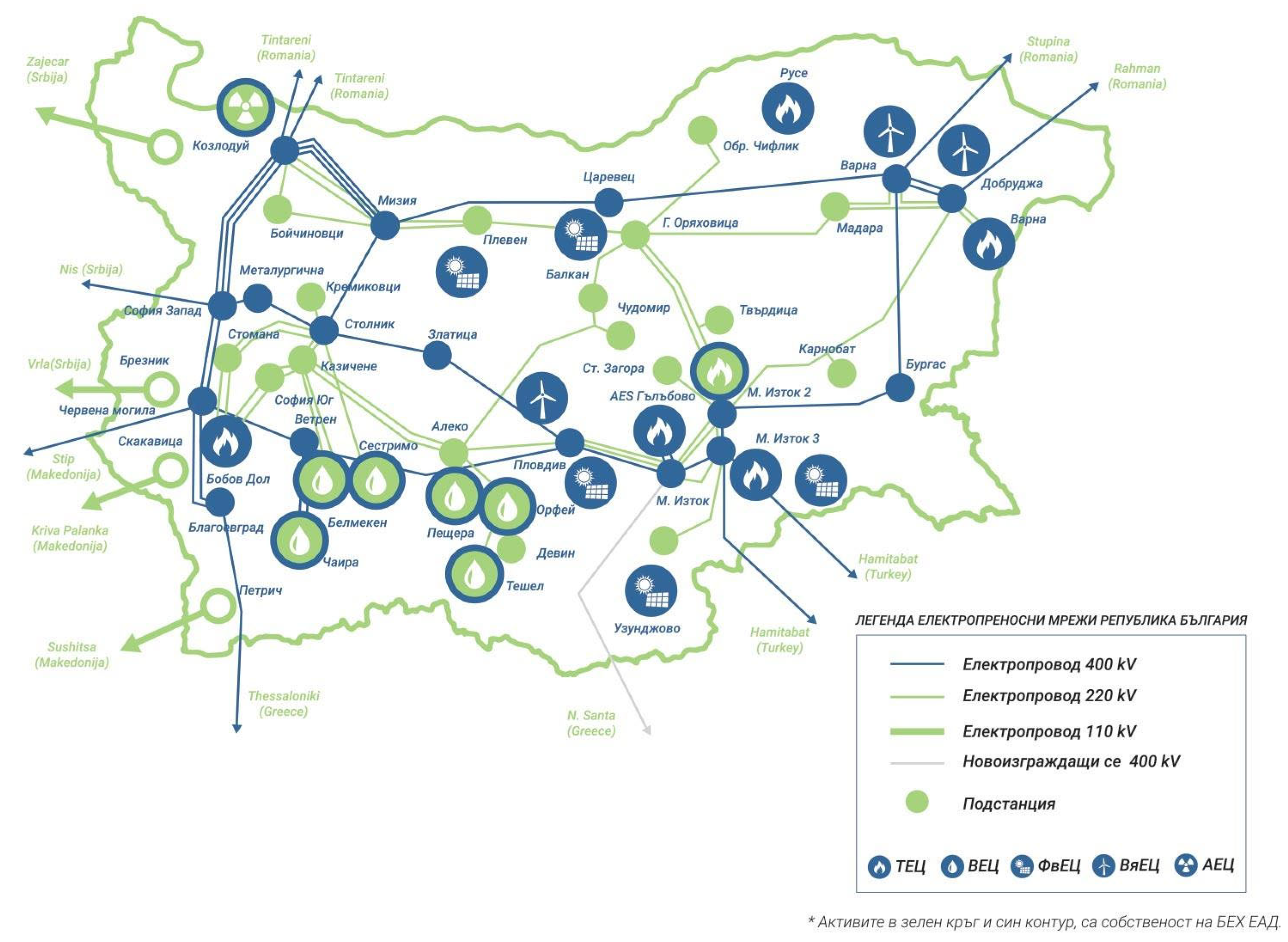
This trend is rising rapidly globally and Bulgaria is no exception. The introduction of renewables to offset the carbon footprint and the privatization of electricity generation plants is leading to a grid transformation from a state-owned centralized dispatchable grid to a decentralized non-dispatchable one. Figure 1 and Figure 2 show what the energy grid used to be without decentralization and the current state.

Currently the electricity mix is supplemented by nearly 4.5 GWp [3], officially, and unofficial estimates of over 6 GWp of installed photovoltaic (PV) plants, which is two to three times the capacity of the Nuclear Power Plant in Kozloduy, depending on the estimate. Peak load for Bulgaria is around 7500 MW in winter months. Peaks in spring and summer when PV plants operate at or near their maximum are around 4500 MW—significantly less than the total installed PV capacity. A number of different PV installations exist depending on their relationship to the grid.

• Feed-in based only, which feeds their energy into the grid with no on-site consumption.
• PV plants used to offset the electricity bill are connected to the grid but do not export excess energy.
• PV plants with feed-in capability and on-site self-consumption.

Common between all types of PV plants is the fact that they reduce the demand for energy coming from traditional plants, like thermal, water and nuclear, either by increasing supply or decreasing demand.

Figure 1. Map of the Bulgarian energy grid showing main transmission lines along with main power plants. Note: The energy ring is formed to provide redundancy. Note: Names on the map are power plants with pictures depicting the primary energy source. Green dots are substations, while power lines are colored as follows: 400 kV—blue, 220 kV—green (thin line), 110 kV—green (thick line), 400 kV (under construction)—light purple. Names of power stations and power lines are in italics in Cyrillic (irrelevant to the study). Glyph icons in the bottom of the legend table are as follows from left to right—Thermal Power Plant, Hydroelectric Power Plant, Photovoltaic Power Plant, Wind farm, Nuclear Power Plant [4].

Figure 1. Map of the Bulgarian energy grid showing main transmission lines along with main power plants. Note: The energy ring is formed to provide redundancy. Note: Names on the map are power plants with pictures depicting the primary energy source. Green dots are substations, while power lines are colored as follows: 400 kV—blue, 220 kV—green (thin line), 110 kV—green (thick line), 400 kV (under construction)—light purple. Names of power stations and power lines are in italics in Cyrillic (irrelevant to the study). Glyph icons in the bottom of the legend table are as follows from left to right—Thermal Power Plant, Hydroelectric Power Plant, Photovoltaic Power Plant, Wind farm, Nuclear Power Plant [4].

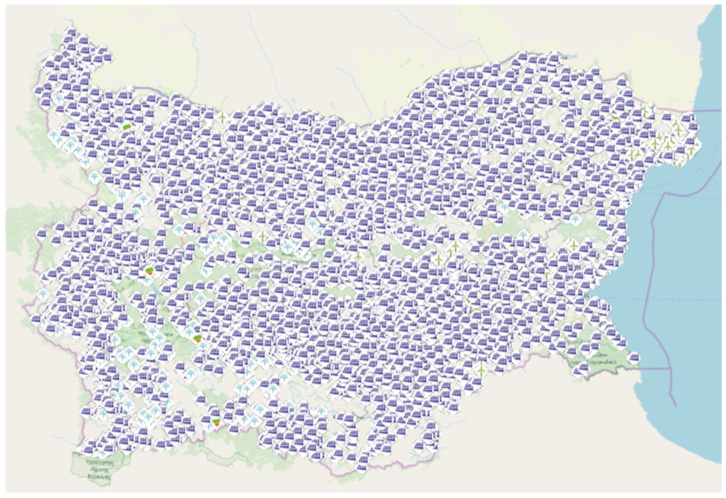
Figure 2. Map of the solar power plants 200 KWp or less distributed across the whole country [5].

Figure 2. Map of the solar power plants 200 KWp or less distributed across the whole country [5].

A major drawback of renewables is that their energy output is heavily dependent on the weather, and their output varies heavily on the availability of the primary energy source; in the case of PV, this is the Sun. Figure 3 depicts the energy production of a 200 kWp PV power plant on a day with dynamic fast-moving clouds.

This is a depiction of the issue with renewables on a microscopic level; at this power the grid can easily absorb power fluctuations of this individual plant. Zoomed out on the macroscopic level, though, the challenge becomes significant. Lost energy at 16:00 must be replaced immediately by another source to keep the service uninterrupted. Since the need for electricity is immediate (the power is required at the instant the light switch is turned on) the following equality must always be met:

Generation − Transmission Losses − Transformation Losses ± Interconnector Flows = Consumption

Any deviation instantly affects grid frequency (target 50 Hz, operational band 49.5–50.2 Hz). In Bulgaria, the Energy System Operator (ESO) is tasked with maintaining the fine balance of generation and consumption to keep the frequency at 50 Hz exact. Frequency is the telltale sign of the amount of energy in the grid. Higher frequency means energy production is higher than demand and vice versa. The operational bound is very narrow as it directly translates to the revolutions per minute that the generators do. Too high and it might turn out that the grid is accelerating the generator shafts. Too low and serious vibrations start to occur which could lead to the destruction of machinery. Traditionally the balance is kept using day-ahead schedules of power plants and consumers. On top of that sits years of experience of weather effects (heating/cooling habits of the population), holidays, special events, etc. The mass adoption of renewables and the “near mandatory” obligation to allow renewables into the grid create an unknown in the amount of dispatchable generation power and to a certain extent on the consumption side as well because of private non feeding, but grid-connected PV plants reduce demand. Approximately 40% of the PV capacity in Bulgaria is connected to the low voltage network meaning no ESO monitoring/control connection is required of the plant.

The physical problem of maintaining that supply/demand problem is translated 1:1 in the financial aspect of the grid operations whereby higher balancing costs would be applied to higher variance generators and vice versa—less balancing with predictable, dispatchable generators.

The current article sets out to introduce a model that would help improve the following three areas:

• Improve balance between generation and load by forecasting PV generation more accurately than traditional theoretical models.
• Increase price paid to Renewable Energy Source (RES) producers by reducing balancing penalties.
• Lower the price paid by consumers through reduced system-wide balancing expenditures charged as grid taxes.

The article shows key findings by the author in the area around these objectives, showing how data-driven individual generation modeling and affordable IoT monitoring together deliver measurable improvements in all three areas.

2. Forecasting Techniques

Accurate forecasting of PV plants is critical to maintain the instantaneous balance that the grid requires to operate and to provide sufficient return on investment (RoI) for developers to encourage further investments in the field. Because solar generation is inherently variable—driven by irradiance, temperature, cloud dynamics, and site-specific factors—forecasting methods have evolved from simple physical calculations to sophisticated data-driven and hybrid approaches. It is important to point out that variance is both weather and installation dependent, so a lot of effort is put into trying to forecast the correct performance from the hourly to the yearly scale [6,7,8]. This section evaluates the main techniques and highlights their strengths and limitations in the context of the big, decentralized fleet of PV power plants in Bulgaria.

2.1. Theoretical Models (TMs)

Note: Some authors refer to these as physical models. These models calculate expected PV output from first principles using meteorological inputs (global horizontal irradiance, direct normal irradiance, diffuse irradiance, ambient temperature, wind speed, geographic location) and plant configuration data (installed capacity, azimuth, tilt, module efficiency, inverter characteristics taken from their datasheet data).

Typically, the calculations are made using tools such as the Photovoltaic Geographical Information System (PVGIS), PVSyst or HelioScope. These tools model the “ideal” power plant within the constraints provided by the design team and integrated planar and weather models.

Significant discrepancies were found however in the analysis of “ideal” sunny days across seasons. Purely theoretical models based on PVGIS inputs showed systematic overestimation, particularly in summer, due to unaccounted temperature-induced efficiency losses (panels reaching 60–65 °C), micro-climatic effects, imperfect orientation and other contributing factors. Cumulative absolute error reached 187.70 MWh annually across the studied plants [9].

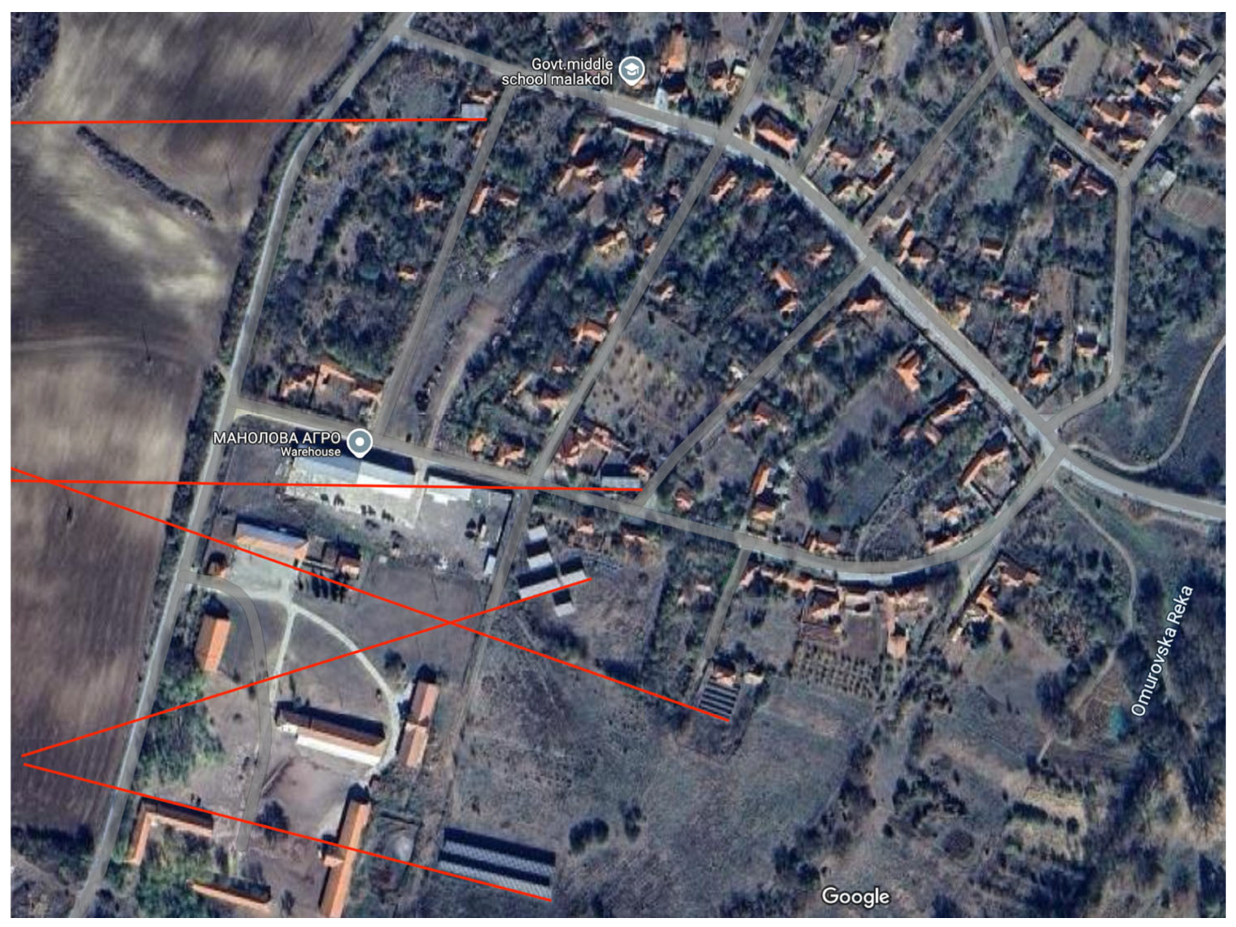
TMs are ideal to get first impressions of the would-be performance of a planned power plant. They require no historical data, and the output is easily interpretable and transparent. However, they lack specific location-based environment factors (e.g., trees, transmission lines, buildings, chimneys, water vapor from nearby lakes or smokestacks, etc.), which are the main contributing factors towards inaccuracies. One of the many installation-specific factors is shown in Figure 4, namely, the azimuth of a few different PV plants, all of which are claimed to be south facing by their respective owner and forecasted as such by the company purchasing energy from them.

2.2. Statistical Models and Time Series

Statistical models rely on historical data and aim to smooth the generation curve to something that is close to the expected result. While they perform reasonably well on the compound energy produced by a lot of small independent generators, they fail to accurately model individual power plants, again due to location- and installation-specific environmental factors. Some of the most common models are:

• Autoregresive Integrated Moving Average (ARIMA) and derivatives (Seasonal Autoregresive Integrated Moving Average (SARIMA), Autoregresive Integrated Moving Average eXogenous (ARIMAX) with weather forecast supplement)
• Various regression techniques.

2.3. ML Models

ML models have become the dominant tool behind the mass introduction of RES power plants. Their ability to learn complex patterns from past behavior makes them ideally suited to fulfill this role. A lot of examples are shown in the literature to perform extremely well. Only the best outliers are briefly mentioned below:

• Shallow ML: K-Nearest Neighbors (KNN), Support Vector Regression (SVR), Random Forest, Gradient Boosting (XGBoost, LightGBM). These excel when feature-engineered inputs (clear sky irradiance, lagged power, temperature) are available.
• Neural Networks: Artificial Neural Networks (ANN), Recurrent Neural Networks (RNN), Long Short-Term Memory (LSTM) networks—particularly effective for time-series
• Hybrid ML-Physical Models: Combine clear-sky or physics-based irradiance with ML correction layers. These frequently outperform pure theoretical or pure statistical methods, with reported R² values reaching 91–98% in ensemble approaches [10].

The only significant drawback with ML algorithms is the fact that they require a lot of historical information beforehand. A general rule of thumb is “the more the better”. This makes them ideal for power plants that have those records available. For new power plants with little to no historical data on their specific environment and installation, they are not ideally suited.

2.4. The Author’s Individual Historic Model (IHM)—A Practical Data-Driven Alternative

The IHM addresses some of the weaknesses of all models outlined above. The model aims to build an exact model of any power plant including all particularities to a specific power plant, some of which develop over time (e.g., shading from trees, soiling, degradation, etc.). Those include but are not limited to micro-climate, exact shading geometry, panel degradation, orientation deviations of 15–30°, bifacial gains, or east–west “shed” layouts. 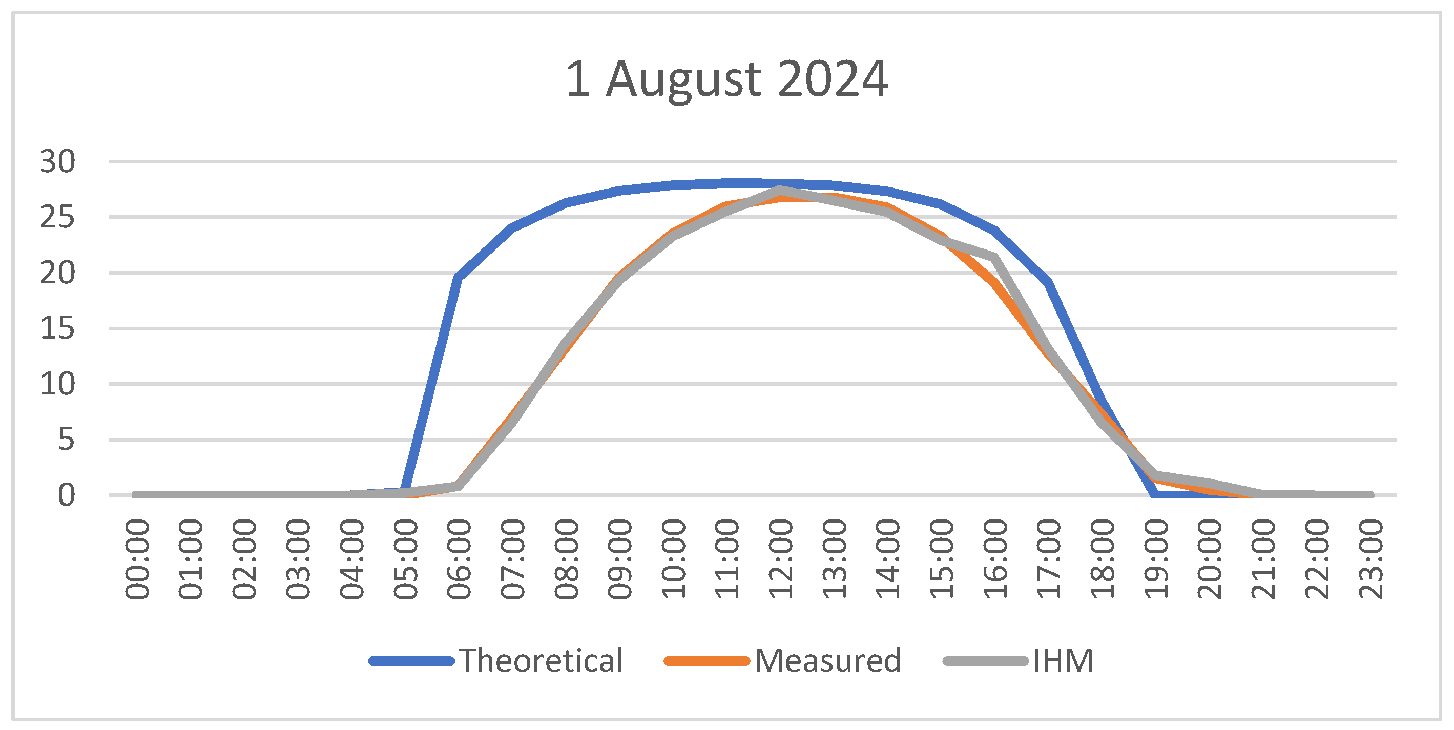Figure 5 shows a comparison between the forecast from PVGIS, which is a TM, IHM forecast built by the author’s model and real-world measured data.

The IHM uses Inverse Distance Weighting (IDW) interpolation on historical 5 min production records of each individual power plant. IDW is an interpolation technique designed to assign more weight to data points that are near in space or time so recent developments (both positive and negative to production) weigh more. The reasoning behind this interpolation is that a lot of factors are subject to change on small private power plants (e.g., shading, soiling, unexpected shutdowns, etc.). The most important bit is that interpolation is done on the same time segment and then those time segments are merged together to form the production curve of the day. This is to some extent because almost all of these plants are geo-distributed in remote areas; there are no maintenance contracts and construction plots are suboptimal. The main driver for most of these installations were subsidized feed-in tariffs by the government so investors rushed to make the deadline, sacrificing ideal location selection. 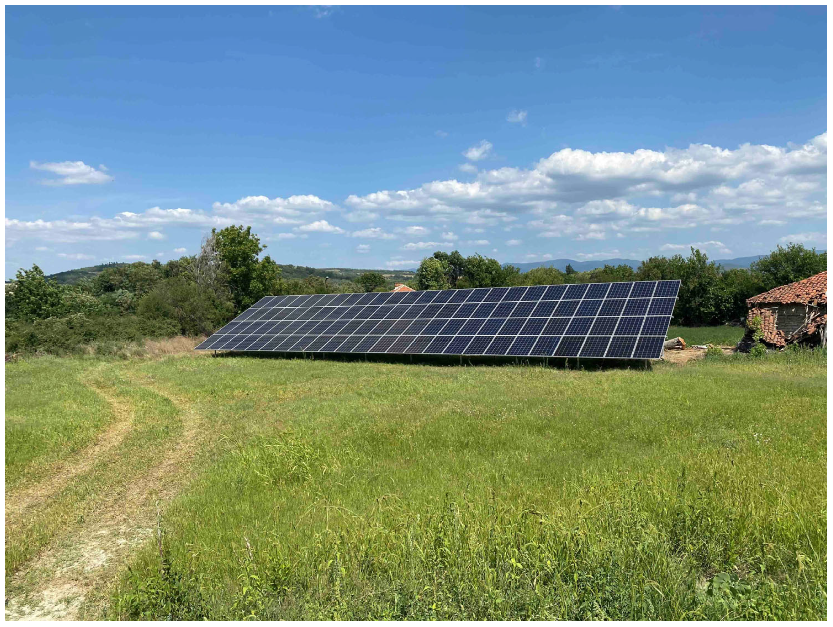Figure 6 and Figure 7 show the difference in execution which translates to a huge performance difference.

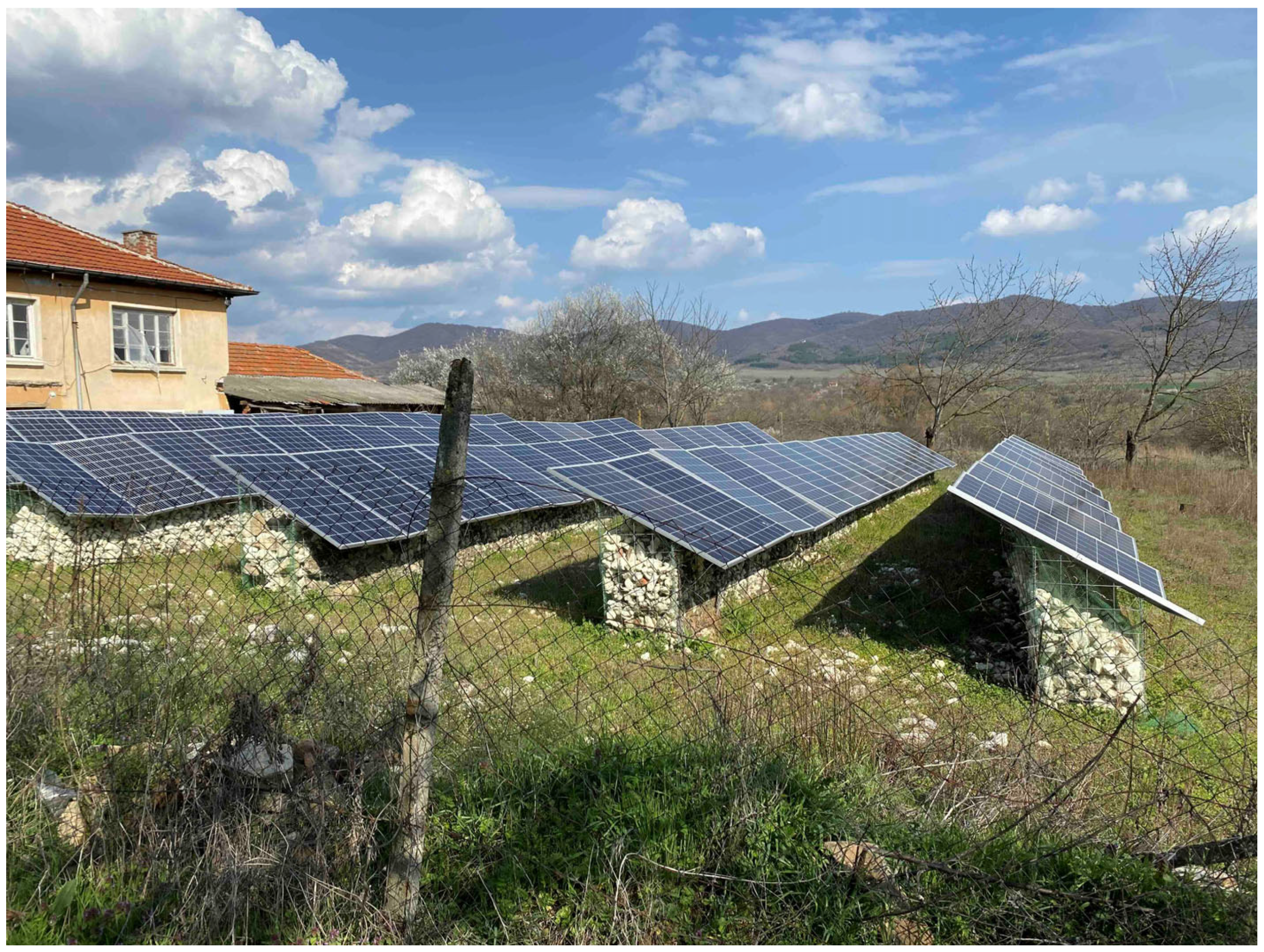
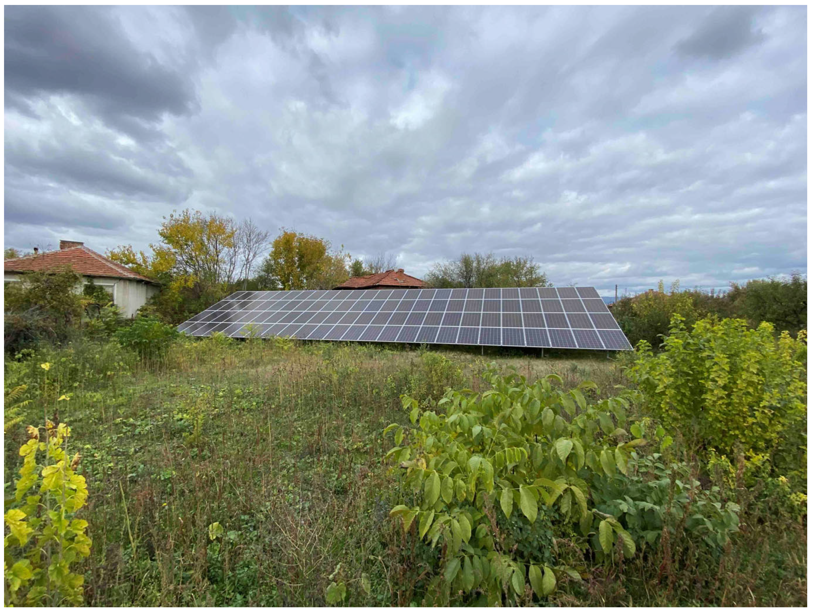
Figure 8 depicts a very good installation; however, overhanging trees and foliage significantly reduce afternoon performance due to shading.

As observed from Figure 4, Figure 6, Figure 7 and Figure 8 there is a big difference in how those plants are executed, oriented and maintained. And this is only in power plants that the author has direct access to as well as performance recording data. The yearly production of the PV plant in Figure 6 is around 32 MWh on a yearly basis, while for the one in Figure 7 it is 46 MWh for the same time period. The one in Figure 8 is in the same plot and same azimuth as Figure 7; however, due to poorer location (note the building on the left) and suboptimal maintenance its yearly production is 42 MWh a year.

What this shows is that even though all three of the plants presented in Figure 6, Figure 7 and Figure 8 are within geographic proximity (less than 1 km apart) and share the same access to their primary energy source and microclimate, their production varies by as much as 30%, in some cases even 45–50%. This makes standard modeling impractical because it is unable to “catch” the peculiarities of each installation.

IHM on the other hand differs from all of the above-mentioned industry standard models in the way that it requires a small amount of data to model a power plant. Post analysis filtering helped reduce the time required to build an accurate model with plant-specific particularities in just 10 days and from then on changes in performance were incorporated into the model. Abrupt disruptions need another 10 days to catch (e.g., string malfunction); however, this is processed by another layer that employs time series ML in the cloud part of the monitoring solution described in Section 3.

The performance observed on four sunny days (1 per season) showed a 4x improvement over regular TM modeling. The error was especially pronounced in surplus forecasting by the TMs. This means that whenever a TM model would forecast more, the IHM would correct with a more accurate lower number.

This leads to reduced balancing costs that are incurred by the producer. A smaller need for balancing the grid results in smaller grid taxes applied to the consumer.

3. Monitoring Solution

The author has developed and put on the market an affordable paid monitoring and control solution to help gather the needed data in order to build accurate modeling for those power plants. Since its introduction there are more than 9 million records of over 60 power plants ranging from 30 kWp to 200 kWp.

The solution is a GSM-based modem with RS485 communication to allow inverter data to be collected. Further down the line, data is sent to the cloud where it is stored and processed. The GSM solution was selected over other communication protocols because of the availability of constant power and signal coverage. SIM cards being used are used in roaming mode to allow connectivity to remote locations.

The system polls the power plants every 5 min during the daytime and every 15 min during night hours. Data is collected by polling the inverter’s internal measuring tooling. Data is considered accurate and is processed as is, apart from simple input validation.

The system notifies customers of any issues it detects using machine learning techniques as well as fixed rules. Daily production emails are also sent to all customers.

The interface of the monitoring solution is shown in the Supplementary Materials (the interface is in Bulgarian).

The data gathered supports the conclusion that the IHM performs better than TMs and statistical models in modeling individual power plant performance. IHM excels in creating a “digital twin” of the power plant, factoring in all location-specific inefficiencies that would otherwise be missed by standard theoretical or statistical models. It also adapts quickly to changes, which is an advantage over some of the machine learning models. The area is rapidly developing a moderate claim over machine learning models.

4. Financial Impact

Financial impact is governed heavily by individual contracts between power companies and power producers. The following data is observed.

Current balance figures in the over-forecasting direction are 11%. This means that power companies forecasted 11% more energy than what was available, which requires them to purchase that 11% difference at elevated prices in order to achieve their day-ahead schedule submitted to ESO.

In terms of under forecasting, the number is 7%. This means that power companies sold 7% more power than they delivered. In this case ESO must either limit power generation under its control or increase demand if possible (e.g., pumped storage if available).

Both these numbers are reduced using the IHM. In terms of over forecasting, regression testing showed an achieved result of 3.4% instead of 7% and in terms of under forecasting the results of the regression tests showed 1.53% versus 11%.

Except for contracts that have fixed balancing, which are gradually being phased out, the effect of using IHM is present and visible. It is impossible to determine the exact improvement due to varying contractual agreements between producers and power companies.

In terms of benefits for consumers, lower balancing needs directly translate to less need to keep dispatchable power plants on hot stand-by, directly reducing costs. It is, however, government good-will to translate those reduced costs into actual savings to consumers.

5. Conclusions

The article shows that standard theoretical modeling provides models that depict near-perfect performance of solar plants which is not always the case in real life, while statistical and machine learning modeling requires a lot of historical data to accurately predict performance and may not catch up with changes on the ground fast enough.

Individual historical modeling proposed by the author can achieve fast modeling of small grid-tied power plants that help reduce balancing costs as well as improve grid stability.

The monitoring solution developed by the author helps collect data needed to gather the data needed to perform the analysis in an affordable and easy-to-use way.

The model shown significantly improves the balancing needed in comparison to what is being used by power companies.