Use of DCC Additional Information for the Expression of Calibration Results in Metrological Practice and Education ^†

Abstract

Technological progress in metrology provides new opportunities for enhancing the quality and transparency of metrological services, with the Digital Calibration Certificate (DCC) playing a significant role in this development. In contrast to traditional calibration certificates, the DCC enables the transfer of extended machine-readable data and can bring additional technical and metrological information describing the calibration process. This paper focuses on the use of DCC additional information for enhanced expression of calibration results in metrological practice and education. Using the example of pressure transducer calibration, the implementation of extended datasets within the DCC structure and their application in result evaluation are demonstrated, including analytical determination of measurement uncertainty and the application of the Monte Carlo method. The results confirm the contribution of DCC to more transparent interpretation of calibration results and to the support of professional education in metrology.

1. Introduction

Calibration certificates are traditionally provided in the form of human-readable documents, most often in PDF format or in paper form. This form limits the further processing of calibration data, as the values must be manually transcribed into calculations software or information systems. Furthermore, in practice, only administrative data and the calibration result are often reported, while further information about the measured data, calibration model or uncertainty components remains hidden in the laboratory’s calculations.

A Digital Calibration Certificate (DCC) offers a solution to this problem. It is a structured data format that allows storing calibration data in a machine-readable format. In addition to the calibration results themselves, other information can be included in the DCC, such as a calibration model, measured (raw) data, or metrological parameters of instrumentation used.

The aim of this paper is to show how additional information stored in DCC can be used in the calculation of measurement uncertainty. Using the example of pressure transducer calibration, it is demonstrated how calibration results can be presented in different ways and subsequently used in the calculation of measurement uncertainty. The work also includes a proposal for the implementation of DCC and its use in the automated processing of calibration results.

The proposed approach is also applied in teaching, namely in practical exercises aimed at measurement technology. Students work with calibration and subsequent measurement with a calibrated measuring instrument. This links the calibration process, evaluation of results, and their practical use in measurement.

2. Materials and Methods

Within the master’s degree study course Measurement in Technology, students complete laboratory exercises focused on the practical implementation of measurements and processing of measurement results. The course also includes calibration of measuring instruments, which are subsequently used in further measurements, allowing students to understand both the measurement process and the importance of calibration.

The output of the exercise focused on the calibration of measuring instruments is the preparation of a calibration certificate, which has so far been provided in PDF form. As part of the innovation of teaching, DCC is being introduced as a structured and machine-readable representation of calibration results.

The proposed DCC will be used in subsequent laboratory exercises, where students will apply calibration results in measurement and uncertainty evaluation. This approach links calibration with practical measurement and supports understanding of uncertainty evaluation in accordance with modern metrological practice.

DCC is currently being addressed by several organizations and many publications deal with it, for example [1,2,3,4]. In general, DCC’s content includes administrative data, measurement description, measurement results and may also include optional content (see

Table 1. DCC content. Adapted with permission from [5]. Copyright 2021, Elsevier Ltd.

Information Block	Description/Examples
Administrative data	Unique identification (ID) of the calibration certificate Calibration provider (student name) Calibration laboratory (school) Customer (teacher)
Measurement results	Measured values (estimate and expanded uncertainty) Units Calibration method and model
Data origin	Equipment used Software used Staff Process description Environmental conditions
Optional content	PDF with results Results of previous calibrations photos of the gauge settings Wiring diagram

).

Currently, the evaluation of calibration is usually carried out in the form of a tabular comparison of the indicated values of the calibrated measuring instrument with the values of the standard. The result is the determination of the deviation and its expanded uncertainty for individual calibration points. These results are subsequently recorded in the calibration certificate. The calibration certificate prepared in this way meets the requirements of the ISO/IEC 17025:2017 standard [6], but the user only gets a limited overview of the performance of the measuring instrument.

In contrast to the classical approach, DCC enables multiple forms of representation of calibration results, which are demonstrated in the following calibration example in Section 3.

3. Calibration Example—Pressure Transducer Calibration

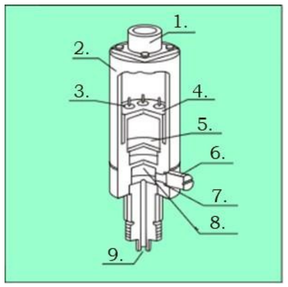
In the practical exercises, students calibrate various measuring instruments. Among other tasks, students perform the calibration of the DMP 333 pressure transducer (see Figure 1) using a standard piston pressure gauge.

According to Figure 1, the transducer consists of connector (1), cover (2), hermetic seal (3), terminals (4), printed circuit board (5), drain valve (6), seal (7), sensitive part of the sensor (8), inlet pressure opening (9).

The pressure is fed into the transducer through the pressure inlet, where it acts on the sensitive part of the sensor. The electrical output signal is fed through the connector to the multimeter and subsequently processed by the calculation software. The metrological properties of the pressure transducer are listed in

Table 2. Metrological properties of the DMP 333 pressure transducer. Reprinted/adapted with permission from [8]. Copyright 2021, BD Senzors GmbH.

Metrological Properties	Value
Type of measured pressure	overpressure
Measuring range	(0–25) MPa
Response time	10 ms
Maximum permissible error	±0.25% of range
Output signal	(4–20) mA

.

The piston pressure gauge, used as a measurement standard for calibration, is traceable to the Slovak national pressure standard in the Slovak Institute of Metrology [9].

Calibration was performed at five calibration points while increasing the pressure and then while decreasing it, to reflect the hysteresis of the gauge.

∆I = I_km,ind − (a + b ∙ (p_et,ind + δp_et)) + δI_kal,mer + δI_kal,stab + δI_kal,tep + δI_hys + δI_zero + δI_rep + δI_repro + δI_multi + δI_roz,mu

(1)

where

∆I—the deviation of the calibrated measuring instrument,

I_km,ind—the indications of a calibrated pressure transducer,

a—the displacement of the calibration line,

b—the slope of the calibration line,

p_et,ind—the indications of the standard,

δp_et—the maximum permissible error of the standard,

δI_kal,mer—the maximum permissible error,

δI_kal,stab—a long-term stability error,

δI_kal,tep—the error due to temperature,

δI_hys—the hysteresis error,

δI_zero—the zero shift error,

δI_rep—the repeatability error,

δI_repro—the reproducibility error,

δI_multi—the maximum permissible error of the multimeter,

δI_roz,mu—the resolution error of the multimeter.

The calibration model (1) expresses the relationship between the pressure value indicated by the calibrated transducer and the pressure value expressed by the standard.

Estimates of measured values are given in

Table 3. Estimates of measured values.

The Indications of the Standard pet,ind/MPa	The Indications of a Calibrated Meter Ikm,ind/mA
0.500	4.323
5.500	7.535
10.500	10.739
15.500	13.940
20.500	17.140
15.500	13.950
10.500	10.748
5.500	7.542
0.500	4.333

.

Estimates of some errors from the calibration model (1) are shown in

Table 4. Influencing variables during calibration. Reprinted/adapted with permission from [8]. Copyright 2021, BD Senzors GmbH.

Error	Error Limit Value δ/MPa	Error Limit Value δ/mA
δpet	0.02% of the estimate	---
δIkal,mer	---	0.056
δIkal,stab	---	0.016
δIkal,tep	---	0.12
δIroz,mu	---	0.0005
δImulti	---	0.007
δIhys	---	0.01

. These data are specified in the technical documentation of the instrument [8].

The data from Table 3 and Table 4 are loaded into the calculation program and the calculation is started.

One possible presentation of calibration results is a classic deviation table (see

Table 5. Influencing variables during calibration.

Measurement Standard Indication pet,ind/MPa	Calibrated Pressure Transducer Indication Ikm,ind/mA	Deviation ∆I/mA	Expanded Uncertainty for k = 2 U/mA
0.5	4.323	0.00	0.155
5.5	7.535	0.015	0.155
10.5	10.739	0.019	0.155
15.5	13.940	0.020	0.155
20.5	17.140	0.020	0.155
15.5	13.950	0.030	0.155
10.5	10.748	0.028	0.155
5.5	7.542	0.022	0.155
0.5	4.333	0.01	0.155

), with uncertainty calculated using the GUM (Guide to the Expression of Uncertainty in Measurement) method.

The other option for presenting the calibration results is the use of a polynomial, whose parameters must be determined during calibration. For the pressure transducer, a first-degree polynomial is employed (see

Table 6. Calibration results presented in the form of first-degree polynomial parameters y = a + bx.

Parameter	GUM Results	Monte Carlo Results
a	4.01179	4.01179
u(a)	0.0449464	0.04492
b	0.640756	0.640751
u(a)	0.00392183	0.00391886
u(a,b)	−0.819167	−0.82043

).

In this case, we can calculate the curve parameters in two ways—analytically by a GUM method and numerical Monte Carlo simulation. Note that the polynomial parameters calculated using both methods are practically identical. Therefore, for the sake of comparison, they are given in Table 6 to a larger number of decimal places.

In addition to tables, the calibration results are also saved in .XML format so that they can be used later in calculating measurement uncertainty.

3.1. Measurement Using a Calibrated Meter

In the next exercise, we measured the pressure with a calibrated gauge and used the calibration results mentioned in Chapter 3 to calculate the measurement uncertainty. The readings are listed in

Table 7. Indications when measuring with a calibrated meter.

i	The Indications of a Calibrated Pressure Transducer Iind/mA
1	10.112
2	10.100
3	10.354
4	10.258
5	10.354
6	10.125
7	10.025
8	10.254
9	10.152
10	10.244

.

During the measurement, several errors may occur that would affect the measurement. However, these errors relate to the calibrated meter and are included in the calibration calculation. First, we calculate the measurement uncertainty using the deviation from Table 5. We select the largest deviation, add the expanded uncertainty to it, and use it in the calculation instead of the maximum permissible error specified by the manufacturer with a uniform distribution => 0.030 mA + 0.155 mA = 0.185 mA. For this evaluation case, we use the following measurement model (2):

I = I_ind + δ_mer,

(2)

where

I—the measured value in mA,

I_ind—the current is indicated in mA,

δ_mer—the meter error determined by calibration in mA.

Table 8. Uncertainty balances for the first calculation method.

Parameter	Estimate	Standard Uncertainty	Distribution	Sensitivity Coefficient	Contribution to Uncertainty	Index
Iind	10.1978 mA	0.0353 mA	Normal	1.0	0.035 mA	9.8%
δmer	0.0 mA	0.107 mA	Rectangular	1.0	0.11 mA	90.2%
I	10.198 mA	---	---	---	0.112 mA	---

shows the measurement result, which must be converted to pressure using the Formula (3):

p_p = (I − a)/b,

(3)

where

p_p—the converted pressure in MPa,

I—the measured current in mA,

a—the displacement of the calibration line (in our case 4),

b—the slope of the calibration line (in our case 0.64).

In the second calculation of measurement uncertainty, we will use the polynomial parameters calculated by calibration, which are in Table 6, instead of the deviation. Since we have different types of calibration results, we also need to change the measurement model (4):

p = (I_ind − a_k)/b_k,

(4)

p—the measured pressure in MPa,

I_ind—the current is indicated in mA,

a_k—the displacement of the calibration line determined by calibration,

b_k—the slope of the calibration line is determined by calibration.

First, we will use the calibration results obtained by the GUM method. The results are shown in

Table 9. Uncertainty balance table for the second calculation method, the GUM method.

Parameter	Estimate	Standard Uncertainty	Distribution	Sensitivity Coefficient	Contribution to Uncertainty	Index
Iind	10.1978 mA	0.0353 mA	Normal	1.6	0.055 MPa	65.1%
ak	4.0118	0.0449	Normal	−1.6	−0.070 MPa	32.8%
bk	0.64076	3.92·10−3	Normal	−15	−0.034 MPa	2.1%
pGUM	9.6542 MPa	---	---	---	0.0682 MPa	---

.

To compare the GUM and Monte Carlo methods (MCM), the same calculation was performed using calibration results obtained by both approaches. The results obtained by the MCM were found to be in good agreement with those obtained by the GUM method. A comparison of the evaluations of measurement results with a calibrated measuring instrument, using both the calibration table and a first order polynomial with parameters obtained by the GUM and MCM, is summarized in

Table 10. Summary of measurement results with calibrated measuring instrument.

Parameter	Estimate p/MPa	Expanded Uncertainty U/MPa
pp	9.6844	0.35
pGUM	9.6542	0.1364
pMC	9.6543	0.1362

.

3.2. Preparation for the Implementation of DCC in Metrological Practice

Implementing DCC into metrological practice requires a systematic approach to processing and organizing data generated during the calibration process. Therefore, the use of DCC is gradually introduced in the exercises to familiarize students with working with digital metrological data and their subsequent use in measurement.

The transition from a classic calibration certificate to DCC represents a significant step in the digitalization of metrology services. Unlike the common PDF, which is intended only for human reading, DCC is designed as a data format enabling automated data processing.

In order to generate a DCC, it is therefore necessary to define the set of input data describing the calibration process.

The basic input data required for creating a DCC include:

• ID of the calibration certificate;
• Calibration laboratory and customer ID;
• ID of the calibrated measuring instrument and standard;
• measured values of the calibrated measuring instrument and standard;
• environmental conditions;
• calibration model;
• calibration results.

Although the structure of the input data for DCC can be defined relatively clearly, its practical implementation into the calibration process requires a systematic approach. It is necessary to consider how the data are obtained, processed and subsequently stored in the digital calibration certificate.

For this reason, the process of introducing DCC was structured using the PDCA (Plan–Do–Check–Act) cycle, as described in greater detail in

Table 11. PDCA cycle.

Plan	Do	Check	Act
methodology proposal	transmitter calibration	analysis of results	implementation proposal
selection of gauge	measurement and calculation of calibration results	comparison of calibration results forms	DCC data structure
definition of calibration model	determination of the expanded uncertainty of deviations	data evaluation	recommendations for practice
input identification	forms of presentation of calibration results	---	---

.

The Plan phase includes the design of the calibration methodology, selection of a suitable measuring instrument, and definition of the calibration model. This phase also includes the identification of input data for processing the calibration results and their subsequent storage in the DCC.

In the Do phase, the actual calibration of the pressure transducer is carried out. It includes measurements at defined calibration points, calculation of calibration results and preparation of various forms of presentation of calibration results.

The Check phase is focused on analyzing the obtained results, comparing different ways of presenting calibration results, and evaluating the calibration results.

In the last phase of Act, DCC implementation procedures and its structure are designed based on the knowledge gained.

When implementing DCC, it is necessary to ensure the processing of data from various sources. In addition to the calibration results themselves, it is also necessary to process administrative data about the measuring instrument, the customer and the equipment used, as well as measured data together with influencing variables.

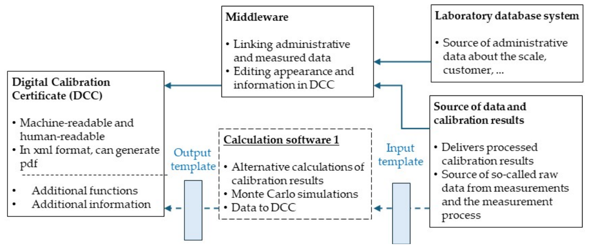
This data must then be processed by computational software and transformed into a structured DCC form. The data processing scheme for creating a DCC is shown in Figure 2.

Figure 2 shows the data processing process leading to the creation of a DCC. Administrative data about the calibrated measuring instrument and the customer are retrieved from the laboratory database. At the same time, the calibration results and raw data obtained during the measurement are also included in the processing process.

These data are then processed by our own calculation software developed in Python 3.13 (2024), which allows for various methods of evaluating calibration results, including alternative calculations or numerical simulations, such as the Monte Carlo method. The middleware layer combines administrative data and calibration results and transforms them into a structured form of DCC, which can be stored in a machine-readable format, such as XML, and can also generate a readable form in PDF format. The calibration results from Chapter 3 were also calculated using this calculation software.

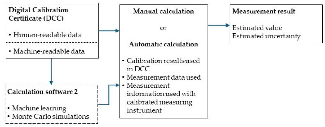
The diagram in Figure 2 describes the process of creating a DCC from the obtained measured and administrative data. In the next step, the DCC created in this way is used as a data source in the measurement processing. The method of using the data stored in the DCC in the measurement evaluation is shown in Figure 3.

The input element in the proposed scheme is the DCC, which contains both human-readable and machine-readable data. The machine-readable part of the DCC allows for its direct processing by computing software without the need for operator intervention.

The calculation of the measurement result can be carried out in two ways—manual or automatic calculation. In the manual calculation, human-readable data is used, which the operator manually writes into the calculation of the measurement uncertainty. In the case of automatic calculation, however, the data from the DCC are processed directly by the software module, which represents another output of this work.

The proposed calculation software allows the use of calibration results stored in the DCC, indications obtained during the measurement and additional influencing variables. Based on these inputs, the measurement result is calculated in the form of an estimate of the value of the measured variable together with the corresponding uncertainty of the estimate.

4. Discussion

The main benefit of this work is the proposal of a methodology using additional DCC information for processing calibration results. The proposed approach allows storing not only the calibration results themselves, but also additional information, including the calibration model and raw data, within the DCC structure. This enables machine-readable processing of the stored data and creates conditions for automated use of calibration results in subsequent measurements.

Another benefit of this work is the implementation of the proposed calibration evaluation methodology into the teaching process. Students thus work with different methods of calibration evaluation, while monitoring their impact on the calculation of measurement uncertainty. This approach contributes to a better understanding of the importance of calibration and its results in practical measurements.

The work also demonstrates a possible transition from a classic calibration certificate in the form of a human-readable document to a DCC containing machine-readable data. This transition is illustrated by the example of a pressure transducer calibration, where it is shown how the calibration results can be stored, processed and subsequently used in further measurements. Similar approaches have also been reported in [10,11,12].

An important goal of this work is also the presentation of various ways of expressing calibration results, which can be part of additional information in DCC. In addition to the classic deviation table, calibration results can also be presented in the form of polynomial parameters. Such extended information allows for more flexible use of calibration results in calculating measurement uncertainty.

In the presented example, the use of polynomial parameters enabled direct application of the calibration model in the measurement evaluation. The results obtained using the GUM and MCM showed very close agreement, with differences on the order of 10⁻⁴ MPa, confirming the consistency of both approaches.

At the same time, the measurement evaluation based on polynomial parameters resulted in a significantly lower uncertainty compared to the use of tabulated deviations, as shown in Table 10, where the expanded uncertainty decreased from approximately 0.35 MPa to 0.136 MPa. The DCC enables full digitalization of metrological traceability by minimizing information loss between calibration and subsequent data processing, thereby improving transparency and the reproducibility of uncertainty evaluation. Overall, the systematic integration of calibration data, models, and uncertainty evaluation in digital form represents a significant step toward modern digital metrology. It also demonstrates the practical applicability of DCC not only in industrial practice but also in the education of future metrologists.

5. Conclusions

The study demonstrates that the use of additional information in DCC significantly enhances the clarity, transparency, and reliability of calibration result presentation in metrological practice. By integrating extended datasets and supplementary technical parameters, practitioners can perform more accurate and flexible evaluations, including analytical uncertainty assessment and Monte Carlo simulations. The example of pressure transducer calibration illustrates the practical implementation of these capabilities, showing clear benefits for both professional metrology and education. Incorporating DCC additional information not only improves result interpretation but also provides a valuable tool for training future metrology professionals, bridging the gap between theoretical knowledge and practical application. Overall, the findings support wider adoption of DCC as a standard for modern calibration reporting and education in the field of metrology.