Diffusion Field Reconstruction by Image Processing Technique ^†

Abstract

In this work, an image reconstruction technique applied for 2D field problem reconstruction is presented. Diffusion concentration plots, represented as images, are used for inverse field reconstruction in the empty part of the image, inside the problem domain. The image reconstruction technique is based on Green’s function linear system minimization for one- and three-layered data structures, visualized as color images. The reconstruction process is implemented as an iterative numerical procedure for field energy and error minimization. Results on low-resolution image reconstruction for 2D diffusion concentration are calculated and presented. The convergence of the method depending on the feedback correction is considered.

1. Introduction

Image reconstruction and restoration methods involve recovering information from a degraded image version or missing part of the image. These methods use different levels of data models that give an internal relation between pixel distribution and suggested data relations of the known part of the image. The reconstruction methods can be broadly divided into traditional and modern machine learning approaches. Basic traditional methods start with statistical Gaussian distribution models over pixels to obtain deviations from average pixel values compared to their neighbors and/or restoring some possible values from the distribution deviation [1]. They continue with many image interpolation techniques by interpolating pixel values over the missing part of the image or between known pixels by using an interpolation equation as an expected distribution model. These techniques are widely used for basic image processing in a relatively small region of interest for smoothing, zooming, denoising, and filtering directly on a small group of neighboring pixels, but can be applied for large spatial image domain reconstruction, considering a much higher number of inter-pixel relations in the model. The large spatial image domain methods are best performed in spatial frequency techniques such as Fast Fourier Transformation over the entire image.

Modern machine learning approaches nowadays mainly include Convolutional Neural Networks (CNNs) for initial spatial segmentation, encoding and even high-level classification, where the modeling stage is implemented in the CNN architecture and/or in trained classification stage, which reacts to large variations in complex pixel groups [2,3]. Encoding is a reversible process, so once composition and training are complete, it can be used for inverse decoding, where new images or parts of images are composed, based on implemented rules. This can be done automatically or semi-automatically, restoring images without prior knowledge of the missing part, or manually by training the NN classificator with a known database, producing a spatial model. These algorithms have numerous applications, including medical imaging, surveillance, and computational photography. They continue to evolve, leveraging advancements in machine learning and computational power to achieve better solution accuracy and efficiency.

This is not a complete review of image reconstruction methods, but it considers the level of modeling used in the reconstruction process and region of interest in the image. Dealing with image reconstruction as a model-centered numerical procedure directly connects it to inverse field problems and multi-parameter optimization methods. Inverse and optimization algorithms can be applied iteratively in order to obtain faster direct solutions and better solution control in the iteration sequence [4].

A special class of images is physical field visualization images [5,6]. The presented distributions are a result of many predefined factors, such as given differential operator, coefficients, sources, etc., that are inaccessible for us at the stage of field visualization. Restoring or reconstructing parts of such images is a direct inverse problem that can benefit from more computationally efficient image processing techniques, trading it for some field physics consistency.

We present an image reconstruction technique for 2D field problems. Diffusion concentration plots are used for inverse field reconstruction in an inaccessible domain. The reconstruction method is based on Green’s function linear system minimization for one- and three-layered data structures, visualized as color images. Error analysis of reconstructed data is performed.

2. Diffusion Modeling

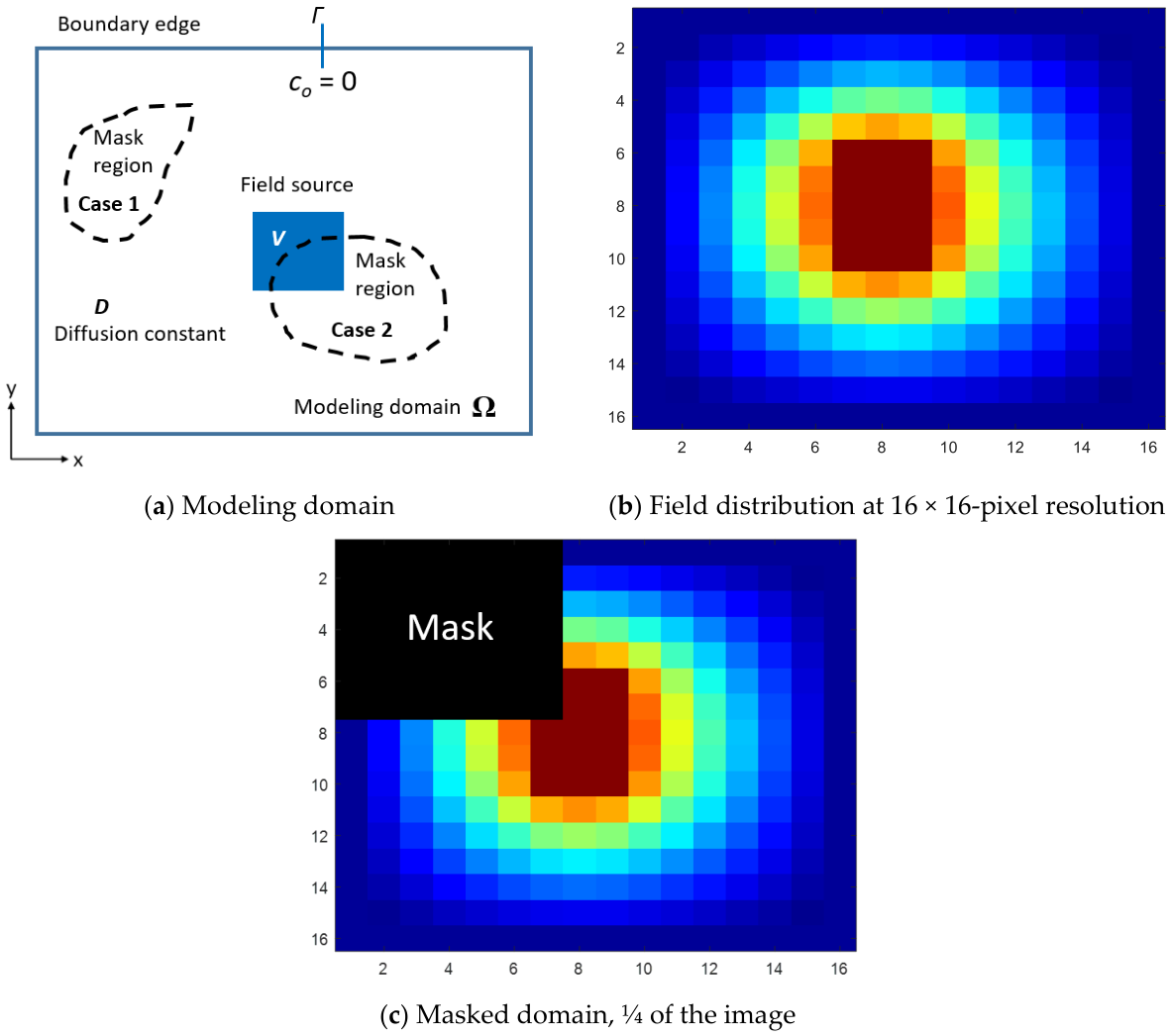
We consider a steady-state diffusion in a closed domain Ω (Figure 1a), described by the Poisson equation, Equation (1),

$${\nabla }^{2}C=-{\displaystyle \frac{v}{D}},$$

(1)

where C is the local gas concentration, D is the diffusion domain constant, v is the source distribution velocity vector, ${\nabla }^2$ is the Laplacian [2]. The solution to Equation (1) in Ω, according to local concentrations C(x, y), can be expressed as Equation (2), where G is the Green’s function, presented by

$$C(x,y)={\displaystyle \frac{1}{D}}{\int }_{\Omega }Gvd\Omega ,$$

(2)

Fluid is situated in the internal cantilever channel and a sequence of pressure pulses are applied on the inlet side (Figure 1b). The outlet is a 0.8 µm hole in the cantilever pyramid end. Droplet formation and position are dependent on fluid flow parameters at the cantilever tip.

The 2D Green’s function for the Laplace operator is expressed as

$$G(r)={\displaystyle \frac{1}{2\pi }}ln(r),$$

(3)

where r is the distance between a given field source at i_x,y and local concentration at j_x,y.

$$r_{ij}=\sqrt{{(x_i-x_j)}^2+{(y_i-y_j)}^2},$$

(4)

3. Field Reconstruction

The concentration distribution in the closed domain Ω at steady state is governed by Equation (1). If the investigated domain is isotropic with constant diffusion coefficient D, the solution can be defined by (2).

The result of the field distribution problem (1) is presented as a color image (Figure 1b). Next, part of the image is removed, as presented in Figure 1c; this part will be restored by the proposed technique.

For image reconstruction, restoration of the masked domain of the concentration field on Figure 1c, the Green’s function is calculated by distance vectors for each mask mesh and complete modeling domain mesh node. After that, a system of linear equations is composed for each local field domain node.

The composed system of linear equations is defined as (5),

M = GX,

(5)

where M is the vector with known values of the concentration, and X are unknown concentrations.

The connectivity matrix G is determined by the local Green’s function G_ij expressions (3) and assembled for each pixel (mesh node) as (6):

$$\mathbf{G}= \left[\begin{array}{ccc}{G}_{11}& \dots & G_{1j}\\ \dots & \dots & \dots \\ G_{i1}& \dots & G_{ij}\end{array}\right] .$$

(6)

The G matrix is symmetric with almost no zero elements. At the next stage, the system of equations is solved by the least square (LS) minimization method. Finally, the X vector is decomposed and distributed on pixel mesh nodes in the masked part of the domain. The method is implemented as a Matlab (R2022a) script program.

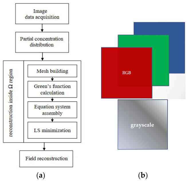
The field reconstruction technique flowchart is presented in Figure 2a. A single iteration of the method is presented. For the iterative implementation, the first reconstructed result is looped back to system assembly and previous iteration results are used as initial concentration distribution in the M matrix. The feedback coefficient controls the previous iteration results in order to obtain solution convergence. For image processing, the technique is applied on each color of the RGB image; three LS minimizations are performed for each of the main colors.

4. Reconstruction Results

The result of field distribution problem (1) is presented as a color image in Figure 1b. Diffusion coefficient D and velocity term v are set to 1 for simplicity. A quarter of the image is removed, as presented in Figure 1c, and this part is the aim of the restoration process by the proposed technique.

The mesh structure repeats the pixel resolution of the image, which is 16 × 16 or a total of 256 pixel nodes for the considered case. The masked part is 7 × 7 pixels or a total of 49 pixel nodes. Each pixel corresponds to a 1 mm distance in the solution x-y coordinate plane.

Two image reconstruction cases are considered: the first is with RGB image coding and the second with grayscale, actually with a single value per pixel. The second case is again visualized as a color image at the end.

Field energy per iteration E_(iter) is calculated by the concentration gradient $\nabla C$ over the image domain Ω (7),

$$E_{(iter)}={\displaystyle {\int }_{\Omega }}D\nabla C^{2}d\Omega ,$$

(7)

Error per iteration is calculated by stepwise energies of sequential iterations (8),

$${Error}_{(iter)}=\left|E_{(iter)}-E_{(iter-1)}\right|,$$

(8)

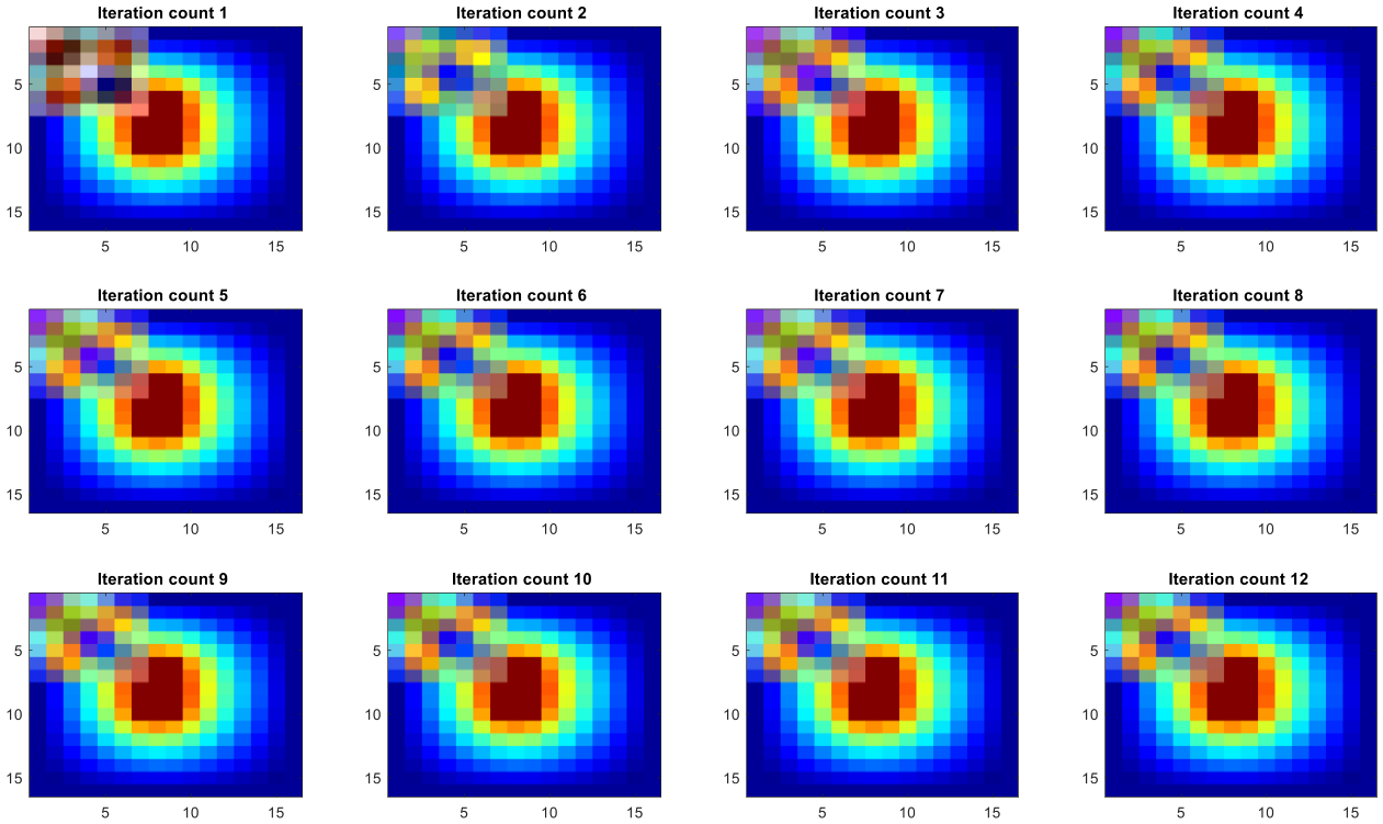
Reconstructed results for the RGB coding case are presented in Figure 3. It shows 12 sequential iterations. The reconstruction process covers 100 iterations, but after the 7th the change is hardly visible. As it can be seen, the reconstruction is not perfect, but it is symmetric and concentration decreases from the center of the image.

The next results are for the grayscale case. The image is again in color only for the visualization. The reconstruction technique is performed on single matrix numerical values and colored only for the visualization.

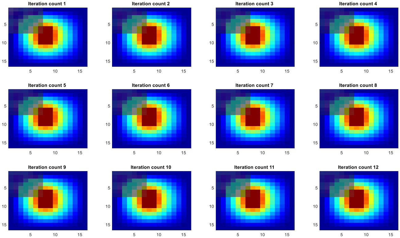
Reconstructed results for the grayscale coding case are presented in Figure 4. As it can be seen, the reconstruction is very good; it is symmetric and concentration decreases from the center of the image. There is a difference with the true values, also visible in the error plots; this may come from the feedback correction coefficient β (Figure 5).

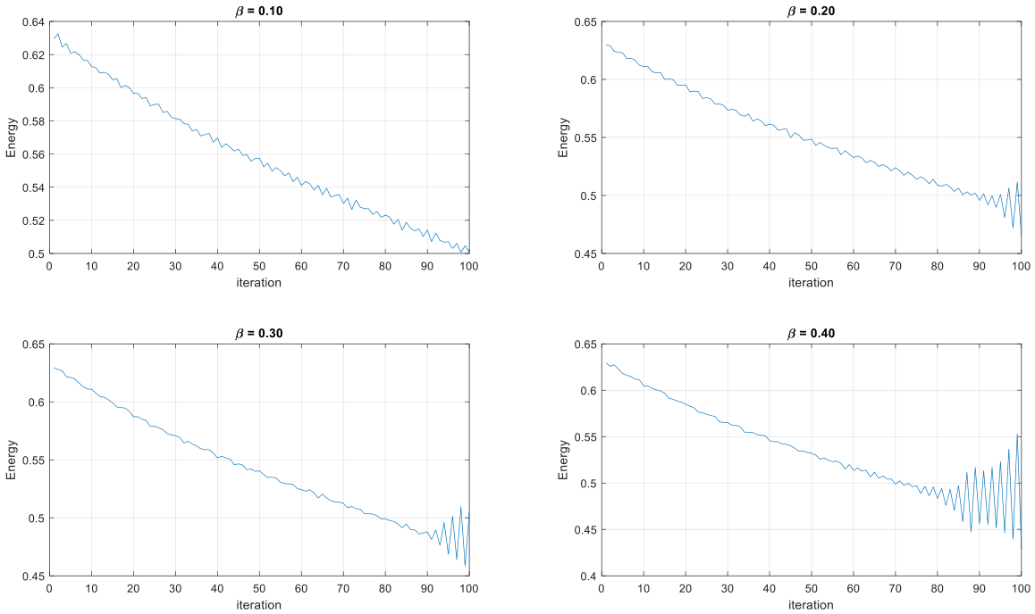
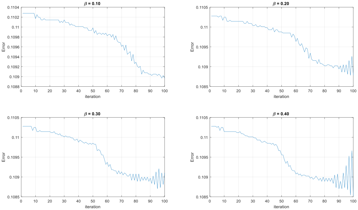
Energy convergence for feedback coefficient β variations from 0.1 to 0.4 is presented in Figure 6. No matter the feedback coefficient, the end convergence is similar for 100 iterations. Some instability is observed for higher coefficients and it starts earlier with higher β numbers. The same instability is observed on error plots in Figure 6, but error convergence is faster with higher β numbers. Values show the convergence step as follows: β = 0.1 (65th iteration), β = 0.2 (60th iteration), β = 0.3 (52nd iteration), and β = 0.4 (46th iteration).

5. Conclusions

An image reconstruction technique for the 2D diffusion concentration field problem is proposed. Diffusion concentration plots are used for inverse field reconstruction in the image domain. The reconstruction method is based on Green’s function linear system minimization for one- and three-layered data structures, visualized as color images. The reconstruction technique directly calculates the concentration distribution without the source reconstruction stage. Feedback coefficient controls the previous iteration results in order to obtain solution convergence. The method shows better accuracy for grayscale image coding, i.e., one numerical value per pixel node. Higher-resolution field images must be processed with this method.

References

- Gunturk, B.; Xin, L. Image Restoration; CRC Press: Boca Raton, FL, USA, 2018. [Google Scholar]
- Mateev, V.; Marinova, I. Fluid flow diffusion modelling with convolutional neural network aided method. AIP Conf. Proc. 2023, 2939, 100009. [Google Scholar] [CrossRef] [Scilit]
- Steffens, C.R.; Messias, L.R.V.; Drews, P.J.L., Jr.; Botelho, S.S.d.C. CNN based image restoration: Adjusting ill-exposed sRGB images in post-processing. J. Intell. Robot. Syst. 2020, 99, 609–627. [Google Scholar] [CrossRef] [Scilit]
- Marinova, I.; Mateev, V. Inverse source problem for thermal fields. Int. J. Comput. Math. Electr. Electron. Eng. COMPEL 2012, 31, 996–1006. [Google Scholar] [CrossRef] [Scilit]
- Romeo, M.; Cottone, G.; D’oca, M.C.; Bartolotta, A.; Gallo, S.; Miraglia, R.; Gerasia, R.; Milluzzo, G.; Romano, F.; Gagliardo, C.; et al. Diffusion Correction in Fricke Hydrogel Dosimeters: A Deep Learning Approach with 2D and 3D Physics-Informed Neural Network Models. Gels 2024, 10, 565. [Google Scholar] [CrossRef] [Scilit] [PubMed]
- Arif, M.Z.; Seppänen, A.; Kolehmainen, V.; Vauhkonen, M. Dual-Modal Electrical Imaging of Two-Phase Flow—Experimental Evaluation of the State Estimation Approach. Sensors 2023, 23, 4462. [Google Scholar] [CrossRef] [Scilit] [PubMed]