Mathematical Models of Systems for Measuring Pressure of Gas–Liquid Media and Their Comparative Analysis ^†

Abstract

The paper considers a linear differential operator and a nonlinear integro-differential operator, on the basis of which the equations of vibration of a deformable plate are written down. The nonlinear operator takes into account the nonlinearity of the longitudinal force arising from the elongation of the plate due to its deformation. Based on the proposed equations, the mathematical models of the mechanical system “pipeline–pressure sensor” are developed. The system consists of a pipeline attached at one end to the combustion chamber of an aircraft engine and a sensor designed to measure the pressure in the combustion chamber at the other end. The sensing element of the sensor that transmits the pressure information is a deformable plate. The models take into account the transfer of heat flow through the pipeline with the working medium (gas or liquid) from the engine to the elastic element and the aerohydrodynamic effect of this medium on the plate. On the basis of the small parameter method, the asymptotic equations describing the joint dynamics of the working medium in the pipeline and the deformable element of the sensor are obtained. The dynamics study is based on the application of the Galerkin method and numerical experiment in Mathematica 12.0. The case of rigid fixation of the elastic element ends is considered. A comparative analysis of solutions for linear and nonlinear models is made. The insignificant influence of the nonlinearity of the longitudinal force on the value of the plate deflection is shown.

1. Introduction

The study of the dynamics and stability of deformable elements is of great importance in the design and operation of structures, devices, and plants for various purposes that interact with the flow of gas or liquid [1,2,3,4,5,6,7,8,9,10,11,12,13,14,15,16,17,18,19,20,21]. In some cases, the impact of the flow can lead to amplitudes, frequencies and velocities of oscillations of elastic elements that do not allow for the reliable operation of systems and do not ensure the functional accuracy of their work. Such a problem arises in the design of pressure sensors. Many works are devoted to the theoretical and practical issues of pressure sensor design. Let us list some of the latest ones [15,16,17,18,19,20,21,22,23,24,25,26,27]. References [17,18,19,20,21,22,23,26,27] are devoted to descriptions of sensors of measuring systems, the principles of their operation, and their technical characteristics. Some works are devoted to describing the materials and manufacturing technologies of sensors [17,18,24].

Pressure sensors operating in aircraft and rocket engines are impacted by high temperatures and increased vibration accelerations, which are most pronounced in transient modes of engine operation. Such extreme operating conditions lead to additional measurement error and even to the destruction of the elastic-sensitive element of the sensor. One of the ways of solving this problem is ensuring the optimal design of the mechanical system “pipeline–pressure sensor”. In this system, the sensor is located some distance from the engine and connected to it by means of a pipeline, which weakens the impact of temperature and vibration accelerations. Mathematical models of the system “pipeline–pressure sensor” were considered, for example, in [15,16].

This paper investigates the joint dynamics of a pressure sensor element and the working medium in a pipeline through mathematical models representing the initial boundary value problems for systems of differential equations. The study of the dynamics of the elastic element applies the Galerkin method and numerical experiments.

This paper studies the influence of the nonlinearity of the longitudinal force arising from the elongation of the pressure sensor-sensing element due to its deformation, based on a comparison of linear and nonlinear models of a solid deformable body, describing the oscillations in the sensor sensing element.

2. Asymptotic Models of Deformable Solid Bodies

In this paper, we study the dynamics of a deformable plate subjected to aerohydrodynamic and thermal effects. Let the deflection of a plate of length $H$ and thickness $h$ depending on the coordinate of the plate point be $y\in [0,H]$, and time $t\ge 0$ is described by the function $w(y,t)$. The case of rigid fixation of the plate ends is considered:

$$w(0,t)=w_y(0,t)=0, w(H,t)=w_y(H,t)=0.$$

(1)

Linear (2) and nonlinear (3) mathematical models of a deformable solid are proposed to describe the plate dynamics:

$$L\left(w(y,t)\right)\equiv M{w}_{tt}+D{w}_{yyyy}+N(t)w_{yy}+\gamma w+{\beta }_1{w}_t+{\beta }_2{w}_{yyyyt};$$

(2)

$$J\left(w(y,t)\right)\equiv L\left(w(y,t)\right)-w_{yy}\left(\mu {\displaystyle {\displaystyle \underset{0}{\overset{H}{\int }}}{w}_y^{2}dy+\eta {\left({\displaystyle {\displaystyle \underset{0}{\overset{H}{\int }}}{w}_y^{2}dy}\right)}_t}\right).$$

(3)

The indices at the bottom denote partial derivatives of the corresponding variables. In operators (2) and (3) the following notations of the mechanical characteristics of the deformed plate are introduced: $M,D$ are the linear mass and bending stiffness of the plate; $N(t)$ is the function describing the compressive or tensile force on the plate; $\gamma$ is the stiffness coefficient of the crimped layer of the plate; ${\beta }_1$ is the coefficient of external damping; ${\beta }_2,\eta$ are the coefficients describing the internal damping of the plate; $\mu$ is the coefficient depending on the strength and geometrical characteristics of the plate. The nonlinear model (3) takes into account the nonlinearity of the longitudinal force resulting from the elongation of the plate due to its deformation.

To calculate the linear mass and bending stiffness of the plate, we use the following formulas:

$$D={\displaystyle \frac{E{h}^3}{12(1-{\nu }^2)}}, M={\rho }_{0}h,$$

(4)

where $E$ is the modulus of elasticity of the plate; $\nu$ is the Poisson’s ratio; ${\rho }_0$ is the density of the plate.

Taking into account the thermal effect on the plate, the variable compressive force coefficient is as follows:

$$N\left(t\right)=N_0+{\displaystyle \frac{E{\alpha }_T}{1-\nu }}{\displaystyle {\displaystyle \underset{0}{\overset{h}{\int }}}T\left(x,t\right)dx,}$$

(5)

where $N_0$ is the constant component of the force created when fixing the plate; ${\alpha }_T$ is the temperature coefficient of linear expansion; $T(x,t)$ is the law of the temperature change along the thickness of the element.

As the plate deformation and the temperature coefficient of linear expansion of the plate material are small, let us represent them in the form of a small parameter $\epsilon ={\displaystyle \frac{h}{H}}$ expansion:

$$w(y,t)=w_0(y)+\epsilon w_1(y,t)+\dots , {\alpha }_T=\epsilon {\alpha }_{T1}+\dots$$

(6)

Restricting to terms of order $\epsilon$, let us represent the operators $L\left(w(y,t)\right), J\left(w(y,t)\right)$ in the following form:

$$L\left(w(y,t)\right)=L_1\left(w_0(y)\right)+\epsilon L_2\left(w_0(y),w_1(y,t)\right), J\left(w(y,t)\right)=J_1\left(w_0(y)\right)+\epsilon J_2\left(w_0(y),w_1(y,t)\right).$$

(7)

Let us introduce the notation $N_1\left(t\right)={\displaystyle \frac{E{\alpha }_{T1}}{1-\nu }}{\displaystyle {\displaystyle \underset{0}{\overset{h}{\int }}}T\left(z,t\right)dz.}$ Then, substituting (6) into (2), (3), we obtain

–

for model (2)

$$\left\{\begin{array}{l}{L}_1\left(w_0(y)\right)=D{w}_{0yyyy}+N_0{w}_{0yy}+\gamma w_0,\\ L_2\left(w_0(y),w_1(y,t)\right)=M{w}_{1tt}+D{w}_{1yyyy} +N_1(t)w_{0yy}+N_0{w}_{1yy}+\gamma w_1+{\beta }_1{w}_{1t}+{\beta }_2{w}_{1yyyyt};\end{array}\right.$$

(8)

–

for model (3)

$$\left\{\begin{array}{l}{J}_1\left(w_0(y)\right)=L_1\left(w_0(y)\right)-\mu w_{0yy}{\displaystyle {\displaystyle \underset{0}{\overset{H}{\int }}}{w}_{0y}^{2}dy},\\ J_2\left(w_0(y),w_1(y,t)\right)=L_2\left(w_0(y),w_1(y,t)\right)+{\beta }_2{w}_{1yyyyt}-\\ -\mu w_{1yy}{\displaystyle {\displaystyle \underset{0}{\overset{H}{\int }}}{w}_{0y}^2(y)dy}-2w_{0yy}\left(\mu {\displaystyle {\displaystyle \underset{0}{\overset{H}{\int }}}{w}_{0y}(y)w_{1y}(y,t)dy+\eta {\displaystyle {\displaystyle \underset{0}{\overset{H}{\int }}}{w}_{0y}(y)w_{1yt}(y,t)dy}}\right).\end{array}\right.$$

(9)

By virtue of the boundary conditions (1) for the function $w(y,t)$, we obtain the boundary conditions for the functions $w_0(y), w_1(y,t)$:

$$w_0(0)=w_{0y}(0)=0, w_0(H)=w_{0y}(H)=0,$$

(10)

$$w_1(0,t)=w_{1y}(0,t)=0, w_1(H,t)=w_{1y}(H,t)=0.$$

(11)

3. Mathematical Model of the Pressure Measurement System

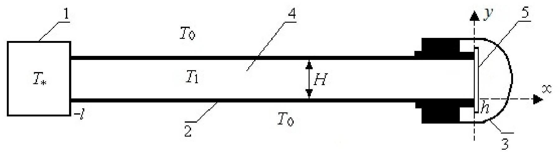
Let the plate be an elastic element in the system for measuring the pressure of the working medium in the combustion chamber of an aircraft engine. The system is shown in Figure 1, where $l$ is the length of the pipeline 2 connecting the pressure sensor 3 with the combustion chamber 1; $T_{*}(t)$ is the law of temperature change at the inlet of the pipeline (at the outlet of the combustion chamber); $T_1(x,t)$ is the law of the temperature change in the working medium along the length of the pipeline 4; $T_2(x,t)$ is the law of the temperature change along the thickness of the element; $T_0$ is the ambient temperature $\left(T_0=const\right)$. We consider a mathematical model of heat flow transmission through a pipeline with a working medium (gas or liquid) from an aircraft engine to a sensor measuring the pressure of this medium. At one end $(x=-l)$ of the pipeline, fixed at the outlet of the engine combustion chamber, there is a change in the pressure of the working medium. At the other end $(x\in [0,h])$ of the pipeline, there is a sensor designed to measure this pressure, the working element of which is an elastic plate 5 The velocity field of the working medium is assumed to be flat.

Let us introduce notations: $\Phi (x,y,t)$ is the velocity potential of the gas–liquid medium; $P(x,y,t)$ is the pressure in this medium; $g(x,y,t)=0$ is the equation of the elastic element surface; $F(y,t)$ is the law of the change in the working medium pressure at the combustion chamber outlet (at the pipeline inlet). Then, the mathematical formulation of the problem in the incompressible medium model is as follows:

$${\Phi }_{xx}+{\Phi }_{yy}=0, x\in \left(-l,0\right), y\in \left(0,H\right),$$

(12)

$${\Phi }_x{g}_x+{\Phi }_y{g}_y=-g_t, g(x,y,t)=0, y\in (0,H),$$

(13)

$$L\left(w(y,t)\right)=P-\overline{P}, y\in (0,H),$$

(14)

$$P=P_0-\rho \left({\Phi }_t+{\displaystyle \frac{1}{2}}{\Phi }_x^2+{\displaystyle \frac{1}{2}}{\Phi }_y^2\right),$$

(15)

$$P(-l,y,t)=F(y,t), y\in (0,H),$$

(16)

$$\rho c_1{T}_{1t}=k_1{T}_{1xx}-\beta \left(T_1-T_0\right), x\in \left(-l,0\right),$$

(17)

$$T_1\left(-l,t\right)=T_{*}\left(t\right),$$

(18)

$$T_{1x}\left(0,t\right)=0,$$

(19)

$${\rho }_0{c}_2{T}_{2t}=k_2{T}_{2xx}, x\in \left(0,h\right),$$

(20)

$$T_{2x}\left(h,t\right)=0,$$

(21)

$$-k_2{T}_{2x}\left(0,t\right)=\alpha {\left.\left(T_1-T_2\right)\right|}_{x=0}.$$

(22)

Here, $P_0$ is the pressure in the resting liquid; $\overline{P}$ is the external pressure on the plate; $\rho$ is the density of the medium; ${\rho }_0$ is the density of the plate material; $k_1,k_2$ are the heat conductivity coefficients of the medium and the plate material, respectively; $c_1,c_2$ are the heat capacity coefficients of the medium and the plate; $\beta$ is the heat exchange coefficient between the pipeline surface and the environment; $\alpha$ is the heat exchange coefficient between the working medium and the plate.

Laplace Equation (12) describes the motion of incompressible medium in the pipeline; boundary condition (13) defines the law of non-flow of gas–liquid medium through the surface of the element; Equation (14) describes the dynamics of the elastic element; pressure in the working medium (15) is determined by the Lagrange–Cauchy integral; Equation (16) defines the law of equality of pressures at the inlet to the pipeline and at the outlet from the combustion chamber of the engine; Equations (17) and (20) describe the law of temperature distribution along the length of the pipeline and along the thickness of the plate, respectively; Equation (18) defines the law of temperature change at the engine outlet; Equation (19) means that the heat flux penetrating through the left boundary of the plate $x =0$ is negligibly small, due to the smallness of the plate thickness and the presence of a vacuum to the right of it; (21) is the thermal insulation of the outer side of the plate, to the right of which there is a vacuum; (22) is the condition of heat exchange between the plate and the working medium in the sensor cavity.

Considering (6), let us write the surface equation of the elastic element in the form

$$g(x,y,t)=x-w(y,t)=x-w_0(y)-\epsilon w_1(y,t)-\dots =0.$$

(23)

Let us represent the functions $\Phi (x,y,t)$, $F(y,t)$ in the form of a small-parameter $\epsilon$ expansion:

$$\Phi (x,y,t)=\epsilon \phi (x,y,t)+\dots , F(y,t)=P_0+\epsilon P_{*}(y,t)+\dots .$$

(24)

where $P_{*}\left(y,t\right)$ is the overpressure at the pipeline inlet (in section $x=-l$).

Substituting (23), (24) into Equations (12)–(16) and restricting ourselves to terms of order $\epsilon$, we obtain an asymptotic model of the problem in the first approximation:

$${\phi }_{xx}+{\phi }_{yy}=0, x\in \left(-l,0\right), y\in (0,H),$$

(25)

$${\phi }_x\left(w_0(y),y,t\right)-w_{0y}(y){\phi }_y\left(w_0(y),y,t\right)=w_{1t}(y,t), y\in (0,H),$$

(26)

$$W_1\left(w_0(y)\right)=P_0-\overline{P}, y\in (0,H),$$

(27)

$$W_2\left(w_0(y),w_1(y,t)\right)=-\rho {\phi }_t\left(w_0(y),y,t\right), y\in (0,H),$$

(28)

$$-\rho {\phi }_t\left(-l,y,t\right)=P_{*}\left(y,t\right), y\in (0,H).$$

(29)

Here, $W_1\left(w_0(y)\right)$, $W_2\left(w_0(y),w_1(y,t)\right)$ is understood as $L_1\left(w_0(y)\right), L_2\left(w_0(y),w_1(y,t)\right)$ for model (2) and $J_1\left(w_0(y)\right), J_2\left(w_0(y),w_1(y,t)\right)$ for model (3).

4. Solving the Problem in the Zero Approximation

Equation (27) is an ordinary differential or integro-differential equation for one unknown function $w_0(y)$ with boundary conditions (10). From (27), we obtain:

–

For model (2)

$$D{w}_{0yyyy}+N_0{w}_{0yy}+\gamma w_0=P_0-\overline{P};$$

(30)

–

For model (3)

$$D{w}_{0yyyy}+N_0{w}_{0yy}+\gamma w_0-\mu w_{0yy}{\displaystyle {\displaystyle \underset{0}{\overset{H}{\int }}}{w}_{0y}^{2}dy}=P_0-\overline{P}.$$

(31)

If the difference between the resting pressure and the external load distributed over the plate is $P_0-\overline{P}=0$, then for each model we obtain $w_0(y)\equiv 0$.

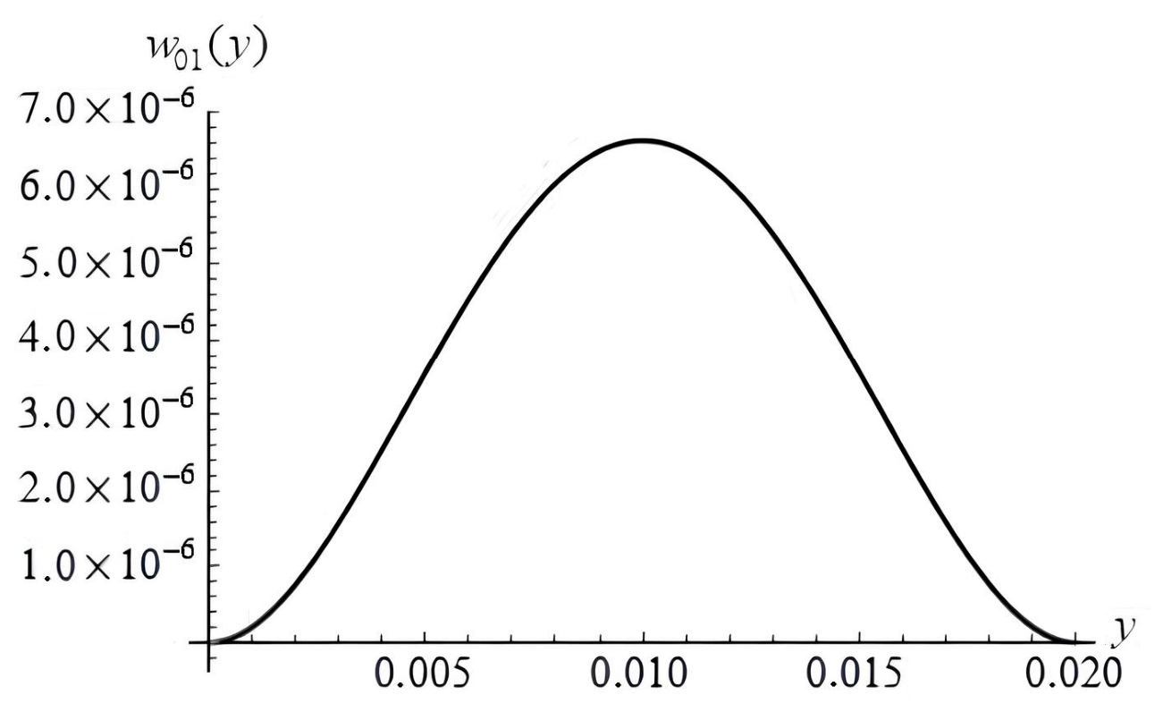
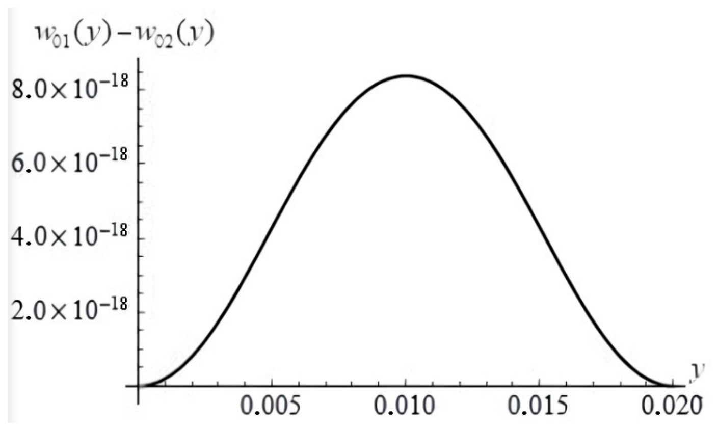
Let us take a non-zero difference $P_0-\overline{P}=2\cdot {10}^4$. Assume that the plate thickness $h=7\times {10}^{-4}$ and length $H=2\cdot {10}^{-2}$ is made of aluminium; then, density ${\rho }_0=2700$, modulus of elasticity $E=7\cdot {10}^{10}$, and Poisson’s ratio $\eta =0.34$. According to (4), $D=2.262,$ $M=1.89.$ Assume that the constant component of the force is $N_0={10}^5$, stiffness coefficient of the crimping layer of the plate is $\gamma =4$, and coefficients at nonlinear terms are $\mu =30$, $\eta =20$. All values are given in SI. In Mathematica 12.0, we numerically find solutions to the boundary value problems in Equations (30) and (31) with boundary conditions (10). The solution of Equation (30) is shown in Figure 2. Figure 3 shows the difference between the solutions of Equations (30) and (31), where $w_{01}(y),w_{02}(y)$ are the solutions of Equations (30) and (31), respectively.

As can be seen from Figure 3, the nonlinear longitudinal force resulting from the elongation of the plate due to its deformation leads to a decrease in the deflection of the plate.

5. Thermal Problem Solving

The solution to the thermal problem (17)–(22) is split into two parts: first the temperature distribution along the length of the pipe is found (Equations (17)–(19)), then the temperature distribution along the thickness of the plate (Equations (20)–(22)).

The solution to Equations (17)–(19) obtained through the separation of variables has the following form:

$$T_1(x,t)=T_{\ast }(t)-{\displaystyle \sum _{n=0}^{\infty }{\chi }_n\cdot e^{-{\gamma }_{n}t}\sin {\nu }_n(x+l)}\left[{\displaystyle \frac{{\beta }^0{T}_0}{{\gamma }_n}}-T_1^0+e^{{\gamma }_{n}t}\left(T_{\ast }(t)-{\displaystyle \frac{{\beta }^0{T}_0}{{\gamma }_n}}\right)-a_1^2{\nu }_n^2{\displaystyle {\displaystyle \underset{0}{\overset{t}{\int }}}{e}^{{\gamma }_n\tau }{T}_{\ast }(\tau )d\tau }\right],$$

(32)

where ${\gamma }_n=a_1^2{\nu }_n^2+{\beta }^0$, ${\nu }_n={\displaystyle \frac{\pi (2n+1)}{2l}}$, ${\chi }_n={\displaystyle \frac{4}{\pi (2n+1)}}$, $T_1^0=T_1(x,0)=const$, $a_1^2={\displaystyle \frac{k_1}{\rho c_1}}$, ${\beta }^0={\displaystyle \frac{\beta }{\rho c_1}}$.

Using Equation (32) it is possible to calculate the temperature at any point on the pipeline at any time t, if the law of temperature change $T_{\ast }(t)$ at the engine outlet is given.

The solution to Equations (20)–(22), which allows us to find the temperature distribution along the plate thickness at an arbitrary moment of time, has the following form:

$$\begin{array}{c}{T}_2(x,t)=\tilde{T}(t)+{\displaystyle \sum _{n=0}^{\infty }{A}_n{e}^{-{\delta }_{n}t}\cos {\mu }_n\left(x-h\right)}\left[T_2^0-T_1^0-{\displaystyle {\displaystyle \underset{0}{\overset{t}{\int }}}{e}^{{\delta }_{n}t}{\tilde{T}}^{\prime }(t)dt}\right]=\\ =\tilde{T}(t)+{\displaystyle \sum _{n=0}^{\infty }{A}_n{e}^{-{\delta }_{n}t}\cos {\mu }_n\left(x-h\right)}\left[T_2^0-T_1^0-{\displaystyle \sum _{k=0}^{\infty }\frac{{\chi }_k\cdot {\gamma }_k\sin {\nu }_{k}l}{{\delta }_n-{\gamma }_k}}\left({\displaystyle \frac{{\beta }^0{T}_0}{{\gamma }_k}}-T_1^0+{\displaystyle \frac{a_1^2{\nu }_k^2{T}_{\ast }}{{\gamma }_k}}\right)\left(e^{({\delta }_n-{\gamma }_k)t}-1\right)\right],\end{array}$$

(33)

where $T_2^0=T_2(x,0)=const$, $a_2^2={\displaystyle \frac{k_2}{{\rho }_0{c}_2}}$, $A_n={\displaystyle \frac{{(-1)}^{n}2\alpha \sqrt{{\alpha }^2+{\lambda }_2^2{\mu }_n^2}}{{\mu }_n\left[h({\alpha }^2+k_2^2{\mu }_n^2)+k_2\alpha \right]}}$, ${\delta }_n=a_2^2{\mu }_n^2$, and the values ${\mu }_n (n=0÷\infty )$ are the positive roots of the following equation:

$$\mathrm{tg} {\mu }_{n}h={\displaystyle \frac{\alpha }{k_2{\mu }_n}}.$$

(34)

The function $\tilde{T}(t)=T_1\left(0,t\right)$ is defined by Equation (32).

Substituting (33), we find the coefficient

$$\begin{array}{c}{N}_1\left(t\right)={\displaystyle \frac{E{\alpha }_{T1}}{1-\nu }}{\displaystyle {\displaystyle \underset{0}{\overset{h}{\int }}}{T}_2\left(x,t\right)dx}={\displaystyle \frac{E{\alpha }_{T1}}{1-\nu }}\left(\tilde{T}(t)h+{\displaystyle \sum _{n=0}^{\infty }\frac{A_n}{{\mu }_n}{e}^{-{\delta }_{n}t}\sin {\mu }_{n}h}\left[T_2^0-T_1^0-{\displaystyle {\displaystyle \underset{0}{\overset{t}{\int }}}{e}^{{\delta }_{n}t}{\tilde{T}}^{\prime }(t)dt}\right]\right)=\\ ={\displaystyle \frac{E{\alpha }_{T1}}{1-\nu }}\left(\tilde{T}(t)h+{\displaystyle \sum _{n=0}^{\infty }\frac{A_n}{{\mu }_n}{e}^{-{\delta }_{n}t}\sin {\mu }_{n}h}\left[T_2^0-T_1^0-{\displaystyle \sum _{k=0}^{\infty }\frac{{\chi }_k\cdot {\gamma }_k\sin {\nu }_{k}l}{{\delta }_n-{\gamma }_k}}\left({\displaystyle \frac{{\beta }^0{T}_0}{{\gamma }_k}}-T_1^0+{\displaystyle \frac{a_1^2{\nu }_k^2{T}_{\ast }}{{\gamma }_k}}\right)\left(e^{({\delta }_n-{\gamma }_k)t}-1\right)\right]\right).\end{array}$$

(35)

Let the medium surrounding the pipeline be air with temperature $T_0=293.15.$ The heat transfer coefficient between the surface of the pipeline and the environment is $\beta =15.5.$ Let us assume that the temperature at the inlet of the pipeline is constant $T_{*}=1800.$ The working medium in a pipeline of length $l=0.5$ and width $H=0.02$ is water, where density $\rho =1000$, heat capacity coefficient $c_1=4182$, and heat transfer coefficient $k_1=0.683$. Assume that the plate thickness $h=7\cdot {10}^{-4}$ is made of aluminium; then, the modulus of elasticity is $E=7\times {10}^{10}$, Poisson’s ratio is $\eta =0.34$, thermal coefficient of linear expansion is ${\alpha }_T=12.3\times {10}^{-6}$, heat capacity coefficient is $c_2=897$, and heat transfer coefficient is $k_2=209.3$. All values are given in the SI system.

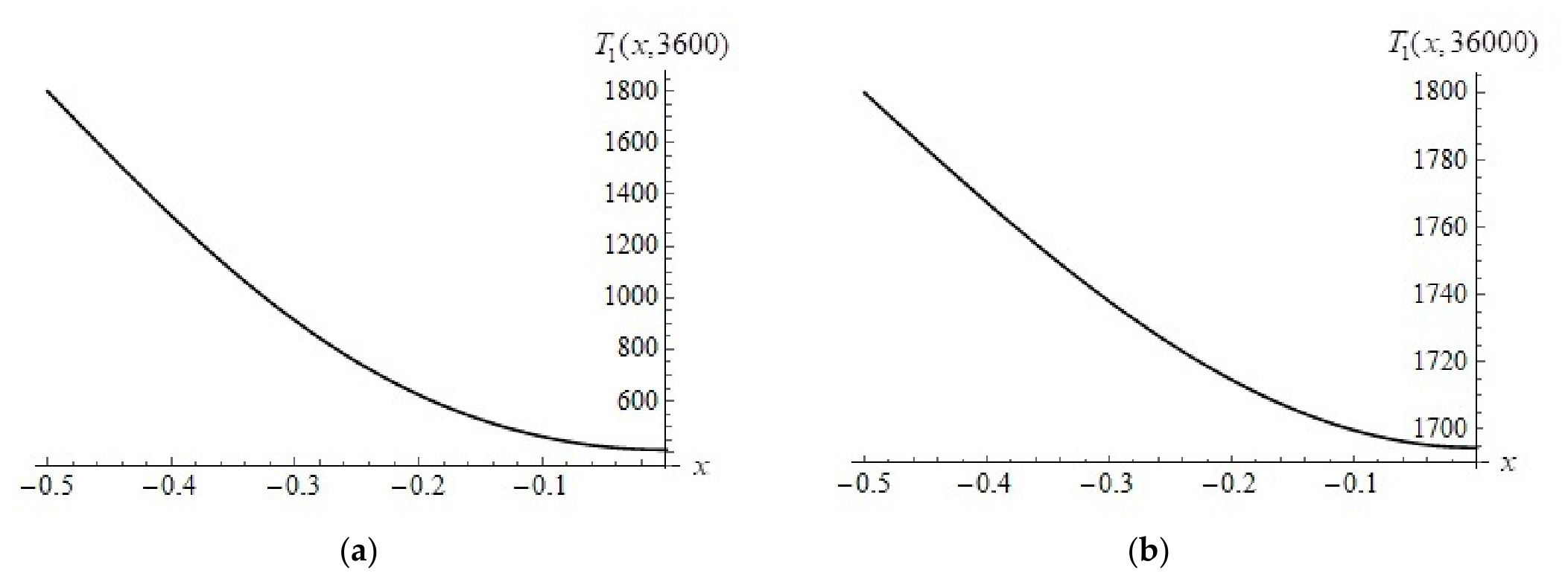
Figure 4 shows the temperature variation along the length of the pipeline.

As can be seen from Figure 4, the temperature of the medium at the boundary with the plate (position $x=0$) starts to increase with time.

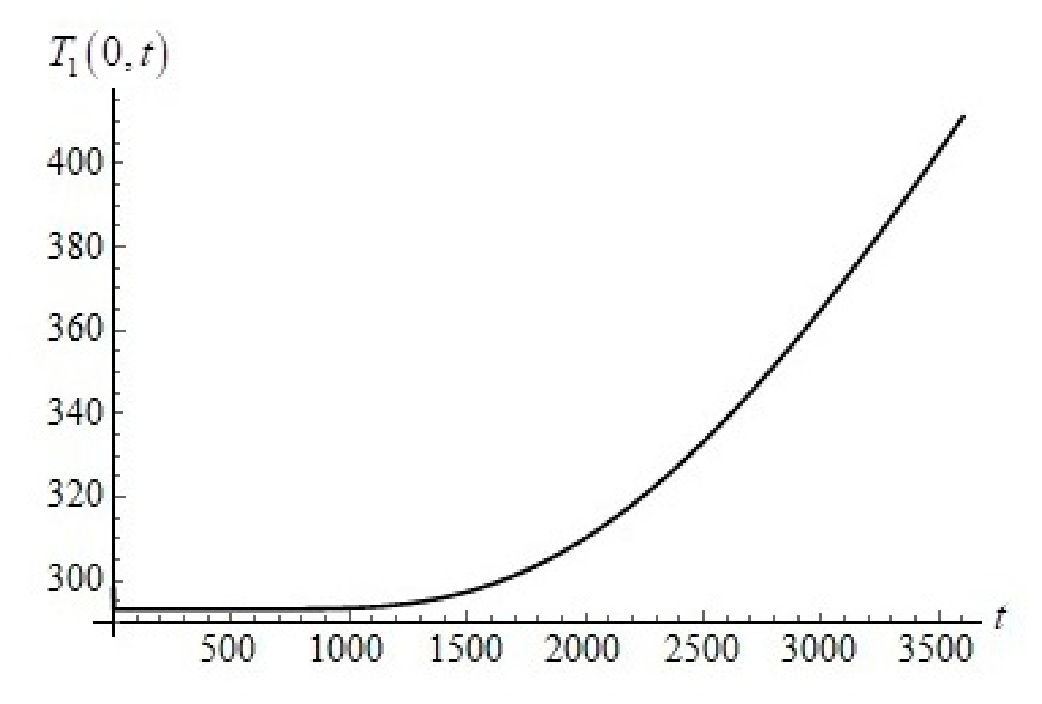
Figure 5 shows the change in the temperature of the working medium at the plate boundary over time $t\in [0,3600]$.

Substituting the found function $\tilde{T}(t)=T_1\left(0,t\right)$, shown in Figure 5, from (35) we obtain the function $N_1\left(t\right)$.

6. Solution of the Aerohydrodynamic Problem

Let us solve the aerohydrodynamic Equations (25), (26), (28) and (29). Assume that the overpressure does not depend on the coordinate $y$, i.e., $P_{*}\left(y,t\right)=P_{*}\left(t\right)$. Then, we will find the potential $\phi (x,y,t)$ in the following form:

$$\phi \left(x,y,t\right)=-{\displaystyle \frac{1}{\rho }}{\displaystyle {\displaystyle \underset{0}{\overset{t}{\int }}}{P}_{*}\left(z\right)dz+\left(x+l\right)\alpha \left(t\right)+{\displaystyle \sum _{n=1}^{\infty }{\phi }_n\left(t\right)\cos {\lambda }_{n}y\cdot \mathrm{sh}{\lambda }_n\left(x+l\right), {\lambda }_n=\frac{n\pi }{H}}}.$$

(36)

Equation (36) satisfies the Laplace Equation (25), Equation (29) and the non-flow conditions on the pipeline walls ${\phi }_y\left(x,0,t\right)={\phi }_y\left(x,H,t\right)=0$. We will look for the function $w_1(y,t)$ in the form of a series expansion over the full system of functions ${\left\{{\xi }_n\left(y\right)\right\}}_{n=1}^{\infty }$ on the segment $\left[0,H\right]$, satisfying the boundary conditions corresponding to the conditions of rigid fixation of the plate ends (11).

According to (11), we will find the function $w_1(y,t)$ in the form

$$w_1(y,t)={\displaystyle \sum _{n=1}^{\infty }{w}_n\left(t\right){\xi }_n\left(y\right)},$$

(37)

where

$${\xi }_n(y)=\mathrm{ch}\left({\mu }_{n}y\right)-\cos \left({\mu }_{n}y\right)-{\displaystyle \frac{\mathrm{ch}\left({\mu }_{n}H\right)-\cos \left({\mu }_{n}H\right)}{\mathrm{sh}\left({\mu }_{n}H\right)-\sin \left({\mu }_{n}H\right)}}\left(\mathrm{sh}\left({\mu }_{n}y\right)-\sin \left({\mu }_{n}y\right)\right),$$

(38)

and ${\mu }_n$ is obtained from the equation $\mathrm{ch}\left({\mu }_{n}H\right)\cos \left({\mu }_{n}H\right)=1$.

Let us substitute (36), (37) into Equation (26).

$$\alpha \left(t\right)+{\displaystyle {\displaystyle \sum _{n=1}^{\infty }}{\phi }_n\left(t\right)\cos {\lambda }_{n}y\cdot {\lambda }_n\mathrm{ch}{\lambda }_n\left(w_0(y)+l\right)}+{\lambda }_n{w}_{0y}(y){\displaystyle {\displaystyle \sum _{n=1}^{\infty }}{\phi }_n\left(t\right)\sin {\lambda }_{n}y\cdot \mathrm{sh}{\lambda }_n\left(w_0(y)+l\right)}={\displaystyle {\displaystyle \sum _{n=1}^{\infty }}{w}_{nt}\left(t\right){\xi }_n\left(y\right)},$$

(39)

According to the Galerkin method, we project (39) onto the complete system of functions ${\left\{\cos {\lambda }_{k}y\right\}}_{k=0}^{\infty }$. Projecting onto the first verification function $\cos {\lambda }_{0}y=1$, we obtain

$$\alpha \left(t\right)\cdot H+{\displaystyle {\displaystyle \sum _{n=1}^{\infty }}{\phi }_n\left(t\right){\lambda }_n{\displaystyle {\displaystyle \underset{0}{\overset{H}{\int }}}\left(\cos {\lambda }_{n}y\mathrm{ch}{\lambda }_n\left(w_0\left(y\right)+l\right)+w_{0y}\left(y\right)\sin {\lambda }_{n}y \mathrm{sh}{\lambda }_n\left(w_0\left(y\right)+l\right)\right)dy}}={\displaystyle {\displaystyle \sum _{n=1}^{\infty }}{w}_{nt}\left(t\right){\displaystyle {\displaystyle \underset{0}{\overset{H}{\int }}}{\xi }_n(y)dy}}.$$

Hence,

$$\begin{array}{c}\alpha \left(t\right)=-{\displaystyle \frac{1}{H}}{\displaystyle \sum _{n=1}^{\infty }{\phi }_n\left(t\right){\lambda }_n{\displaystyle {\displaystyle \underset{0}{\overset{H}{\int }}}\left(\cos {\lambda }_{n}y\mathrm{ch}{\lambda }_n\left(w_0\left(y\right)+l\right)+w_{0y}\left(y\right)\sin {\lambda }_{n}y \mathrm{sh}{\lambda }_n\left(w_0\left(y\right)+l\right)\right)dy}}+\\ +{\displaystyle \frac{1}{H}}{\displaystyle \sum _{n=1}^{\infty }{w}_{nt}\left(t\right){\displaystyle {\displaystyle \underset{0}{\overset{H}{\int }}}{\xi }_n(y)dy}}.\end{array}$$

(40)

Let us introduce the notations

$$A_n={\lambda }_n{\displaystyle {\displaystyle \underset{0}{\overset{H}{\int }}}\left(\cos {\lambda }_{n}y\mathrm{ch}{\lambda }_n\left(w_0\left(y\right)+l\right)+w_{0y}\left(y\right)\sin {\lambda }_{n}y \mathrm{sh}{\lambda }_n\left(w_0\left(y\right)+l\right)\right)dy}, B_n={\displaystyle {\displaystyle \underset{0}{\overset{H}{\int }}}{\xi }_n\left(y\right)dy}.$$

(41)

Then, from (40) we obtain

$$\alpha \left(t\right)=-{\displaystyle \frac{1}{H}}{\displaystyle {\displaystyle \sum _{n=1}^{\infty }}{A}_n{\phi }_n\left(t\right)}+{\displaystyle \frac{1}{H}}{\displaystyle {\displaystyle \sum _{n=1}^{\infty }}{B}_n{w}_{nt}\left(t\right)}.$$

(42)

Projecting (39) onto the remaining functions ${\left\{\cos {\lambda }_{k}y\right\}}_{k=1}^{\infty }$, according to the Galerkin method, we obtain

$$\begin{array}{c}{\displaystyle {\displaystyle \sum _{n=1}^{\infty }}{\phi }_n\left(t\right){\lambda }_n}{\displaystyle {\displaystyle \underset{0}{\overset{H}{\int }}}\left(\cos {\lambda }_{n}y\mathrm{ch}{\lambda }_n\left(w_0\left(y\right)+l\right)+w_{0y}\left(y\right)\sin {\lambda }_{n}y \mathrm{sh}{\lambda }_n\left(w_0\left(y\right)+l\right)\right)\cos {\lambda }_{k}ydy}+\\ +\alpha \left(t\right){\displaystyle {\displaystyle \underset{0}{\overset{H}{\int }}}\cos {\lambda }_{k}ydy}={\displaystyle {\displaystyle \sum _{n=1}^{\infty }}{w}_{nt}\left(t\right){\displaystyle {\displaystyle \underset{0}{\overset{H}{\int }}}{\xi }_n(y)\cos {\lambda }_{k}ydy},} k=1,2,\dots \end{array}$$

(43)

Let us introduce the notations

$$C_{nk}={\lambda }_n{\displaystyle {\displaystyle \underset{0}{\overset{H}{\int }}}\left(\cos {\lambda }_{n}y\mathrm{ch}{\lambda }_n\left(w_0\left(y\right)+l\right)+w_{0y}\left(y\right)\sin {\lambda }_{n}y \mathrm{sh}{\lambda }_n\left(w_0\left(y\right)+l\right)\right)\cos {\lambda }_{k}ydy}, V_{nk}={\displaystyle {\displaystyle \underset{0}{\overset{H}{\int }}}{\xi }_n(y)\cos {\lambda }_{k}ydy}.$$

(44)

Considering that

$${\displaystyle {\displaystyle \underset{0}{\overset{H}{\int }}}\cos {\lambda }_{k}ydy}=0,$$

(45)

from (43), we obtain

$${\displaystyle {\displaystyle \sum _{n=1}^{\infty }}{V}_{nk}{w}_{nt}\left(t\right)}={\displaystyle {\displaystyle \sum _{n=1}^{\infty }}{C}_{nk}{\phi }_n\left(t\right)}, k=1,2,\dots$$

(46)

Hence, from (46) we obtain a system of homogeneous equations

$${\displaystyle \sum _{n=1}^{\infty }\left(V_{nk}{w}_{nt}\left(t\right)-C_{nk}{\phi }_n\left(t\right)\right)}=0, k=1,2,\dots$$

(47)

Let us substitute (36), (37) into Equation (28)

$$W_2\left(w_0(y),{\displaystyle \sum _{n=1}^{\infty }{w}_n\left(t\right){\xi }_n\left(y\right)}\right)=P_{*}\left(t\right)-\rho \left(w_0(y)+l\right){\alpha }_t\left(t\right)-\rho {\displaystyle \sum _{n=1}^{\infty }{\phi }_{nt}\left(t\right)\cos {\lambda }_{n}y\cdot \mathrm{sh}{\lambda }_n\left(w_0(y)+l\right). }$$

(48)

Projecting (48) onto the system of functions ${\left\{{\xi }_k\left(y\right)\right\}}_{k=1}^{\infty }$, according to the Galerkin method, we obtain

$$\begin{array}{c}{\displaystyle {\displaystyle \underset{0}{\overset{H}{\int }}}{W}_2\left(w_0(y),{\displaystyle \sum _{n=1}^{\infty }{w}_n\left(t\right){\xi }_n\left(y\right)}\right){\xi }_k}\left(y\right)dy=P_{*}\left(t\right)\cdot {\displaystyle {\displaystyle \underset{0}{\overset{H}{\int }}}{\xi }_k}\left(y\right)dy-\rho {\alpha }_t\left(t\right){\displaystyle {\displaystyle \underset{0}{\overset{H}{\int }}}\left(w_0(y)+l\right){\xi }_k}\left(y\right)dy-\\ -\rho {\displaystyle \sum _{n=1}^{\infty }{\phi }_{nt}\left(t\right){\displaystyle {\displaystyle \underset{0}{\overset{H}{\int }}}\cos {\lambda }_{n}y\cdot \mathrm{sh}{\lambda }_n\left(w_0(y)+l\right)\cdot {\xi }_k}\left(y\right)dy }, k=1,2,\dots \end{array}$$

(49)

Let us introduce the notations

$$D_k=\rho {\displaystyle {\displaystyle \underset{0}{\overset{H}{\int }}}\left(w_0(y)+l\right){\xi }_k}\left(y\right)dy, E_{nk}=\rho {\displaystyle {\displaystyle \underset{0}{\overset{H}{\int }}}\cos {\lambda }_{n}y\cdot \mathrm{sh}{\lambda }_n\left(w_0(y)+l\right)\cdot {\xi }_k}\left(y\right)dy.$$

(50)

Then, substituting (42), from (49) we obtain

$${\displaystyle {\displaystyle \underset{0}{\overset{H}{\int }}}{W}_2\left(w_0(y),{\displaystyle \sum _{n=1}^{\infty }{w}_n\left(t\right){\xi }_n\left(y\right)}\right){\xi }_k}\left(y\right)dy=B_k{P}_{*}\left(t\right)+{\displaystyle \frac{D_k}{H}}{\displaystyle {\displaystyle \sum _{n=1}^{\infty }}{A}_n{\phi }_{nt}\left(t\right)}-{\displaystyle \frac{D_k}{H}}{\displaystyle {\displaystyle \sum _{n=1}^{\infty }}{B}_n{w}_{ntt}\left(t\right)}-{\displaystyle {\displaystyle \sum _{n=1}^{\infty }}{E}_{nk}{\phi }_{nt}\left(t\right) }, k=1,2,\dots$$

(51)

As a result, we obtain a system of ordinary differential Equations (47) and (51) for determining the unknown functions ${\phi }_n\left(t\right),$ $w_n\left(t\right)$.

7. Numerical Experiment

Let us perform a numerical experiment for models (8) and (9), limiting the number of summands in expansions (36) and (37) to $m$.

Let the medium surrounding the pipeline be air with temperature $T_0=293.15.$ The heat transfer coefficient between the surface of the pipeline and the environment $\beta =15.5.$ Let us assume that the temperature at the inlet of the pipeline is constant $T_{*}=1800,$ and the overpressure is variable $P_{*}(t)={10}^6(5-\cos 10t).$ The working medium in a pipeline of length $l=0.5$ and width $H=0.02$ is water; then, the density $\rho =1000$, heat capacity coefficient $c_1=4182$, and heat conductivity coefficient $k_1=0.683$. Let the difference between the pressure in the resting medium and the external load distributed on the plate be $P_0-\overline{P}=2\times {10}^4$. Suppose that the plate thickness $h=7\times {10}^{-4}$ is made of aluminium; then, density ${\rho }_0=2700$, modulus of elasticity $E=7\times {10}^{10}$, Poisson’s ratio $\eta =0.34$, thermal coefficient of linear expansion ${\alpha }_T=12.3\times {10}^{-6}$, heat capacity coefficient $c_2=897$, thermal conductivity coefficient $k_2=209.3$, bending stiffness $D={\displaystyle \frac{E{h}^3}{12(1-{\nu }^2)}}=2262,$ and linear mass $M={\rho }_{0}h=1.89$. Assume that the constant component of force $N_0={10}^5$, the stiffness coefficient of the crimped plate layer $\gamma =4$, and the other coefficients are as follows: $\mu =30$, $\eta =10$, ${\beta }_1=4$, ${\beta }_2=4$. All values are given in the SI system.

Let us take the initial conditions $T_1^0=293.15,$ $T_2^0=293.15,$ $w_k(0)=0,$ $w_{kt}(0)=0,$ $k=1,\dots ,m$.

Solving the system (47), (51) in Mathematica 12.0, taking the segments of series in the formulas of length $m=8,$ we construct the graphs of the deformation function $w(y,t)=w_0\left(y\right)+\epsilon {\displaystyle \sum _{n=1}^m{w}_n\left(t\right){\xi }_n\left(y\right)}$.

Consider the linear model of a deformable solid (8). Substituting $L_2\left(w_0(y),{\displaystyle \sum _{n=1}^m{w}_n\left(t\right){\xi }_n\left(y\right)}\right)$ into (51), we obtain

$$\begin{array}{c}{\displaystyle {\displaystyle \underset{0}{\overset{H}{\int }}}\left(M{\displaystyle {\displaystyle \sum _{n=1}^{\infty }}{w}_{ntt}\left(t\right){\xi }_n\left(y\right)}+D{\displaystyle {\displaystyle \sum _{n=1}^{\infty }}{w}_n\left(t\right){\xi }_{nyyyy}\left(y\right)} +N_1(t)w_{0yy}+N_0{\displaystyle {\displaystyle \sum _{n=1}^{\infty }}{w}_n\left(t\right){\xi }_{nyy}\left(y\right)}+\gamma {\displaystyle {\displaystyle \sum _{n=1}^{\infty }}{w}_n\left(t\right){\xi }_n\left(y\right)}\right.}+\\ \left.+{\beta }_1{\displaystyle {\displaystyle \sum _{n=1}^m}{w}_{nt}\left(t\right){\xi }_n\left(y\right)}+{\beta }_2{\displaystyle {\displaystyle \sum _{n=1}^m}{w}_{nt}\left(t\right){\xi }_{nyyyy}\left(y\right)}\right){\xi }_k\left(y\right)dy=B_k{P}_{*}\left(t\right)+{\displaystyle \frac{D_k}{H}}{\displaystyle \sum _{n=1}^{\infty }{A}_n{\phi }_{nt}\left(t\right)}-\\ -{\displaystyle \frac{D_k}{H}}{\displaystyle {\displaystyle \sum _{n=1}^{\infty }}{B}_n{w}_{ntt}\left(t\right)}-{\displaystyle {\displaystyle \sum _{n=1}^{\infty }}{E}_{nk}{\phi }_{nt}\left(t\right) }, k=1,2,\dots \end{array}$$

(52)

Let us introduce the notations

$$F_{nk}={\displaystyle {\displaystyle \underset{0}{\overset{H}{\int }}}{\xi }_{nyyyy}\left(y\right){\xi }_k}\left(y\right)dy, J_k={\displaystyle {\displaystyle \underset{0}{\overset{H}{\int }}}{w}_{0yy}{\xi }_k}\left(y\right)dy, G_{nk}={\displaystyle {\displaystyle \underset{0}{\overset{H}{\int }}}{\xi }_{nyy}\left(y\right){\xi }_k}\left(y\right)dy.$$

(53)

Given (41) and the orthogonality of the functions (38) on the segment $[0,H]$:

$${\displaystyle {\displaystyle \underset{0}{\overset{H}{\int }}}{\xi }_n(y){\xi }_k\left(y\right)dy=0}, n\ne k, {\displaystyle {\displaystyle \underset{0}{\overset{H}{\int }}}{\xi }_k^2\left(y\right)dy=H,}$$

(54)

we obtain

$$\begin{array}{c}{\displaystyle \sum _{n=1}^{\infty }\left[\left(MH{\delta }_{nk}+\frac{D_k{B}_n}{H}\right)w_{ntt}\left(t\right)+\left({\beta }_{1}H{\delta }_{nk}+{\beta }_2{F}_{nk}\right)w_{nt}\left(t\right)+\right.}\left(D{F}_{nk} +N_0{G}_{nk}+\gamma H{\delta }_{nk}\right)w_n\left(t\right)-\\ -\left.\left({\displaystyle \frac{D_k{A}_n}{H}}-E_{nk}\right){\phi }_{nt}\left(t\right)\right]=B_k{P}_{*}\left(t\right)-J_k{N}_1(t), k=1,2,\dots \end{array}$$

(55)

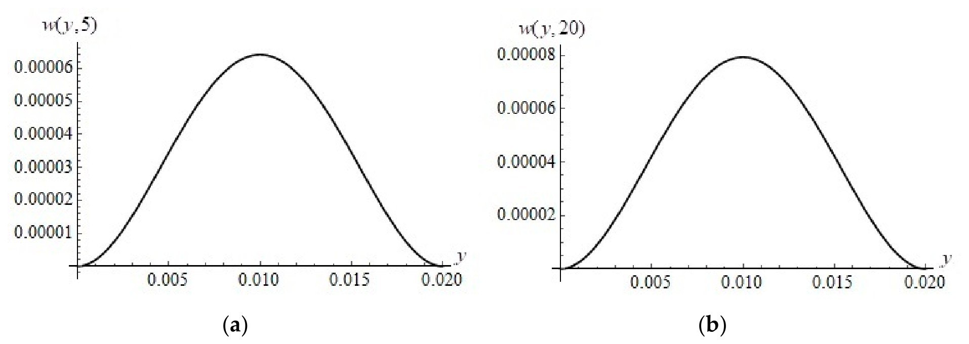
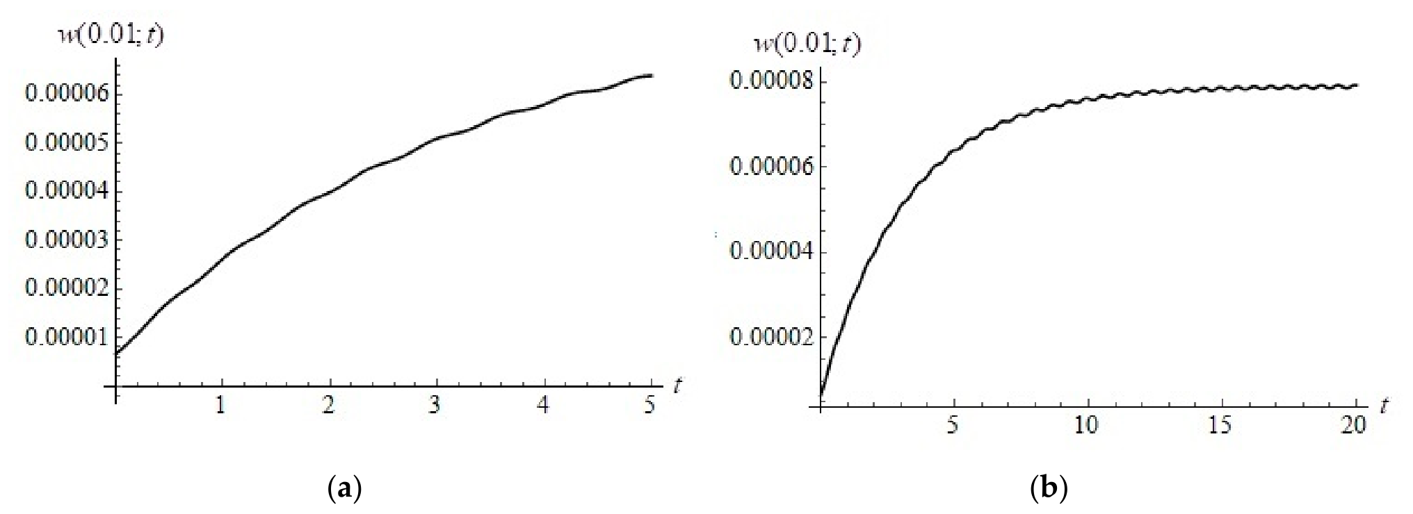
Figure 6 shows the deformations of the plate at time $t=5$ (Figure 6a) and $t=20$ (Figure 6b) at $m=8$. Figure 7 shows the deformations of the plate at the midpoint $y=0.01$ of the plate at $t\in [0,5]$ (Figure 7a) and $t\in [0,20]$ (Figure 7b) at $m=8$.

Let us consider the nonlinear model of a deformable solid (9). Substituting $J_2\left(w_0(y),{\displaystyle \sum _{n=1}^m{w}_n\left(t\right){\xi }_n\left(y\right)}\right)$ into (51), we obtain

$$\begin{array}{c}{\displaystyle {\displaystyle \underset{0}{\overset{H}{\int }}}\left(M{\displaystyle {\displaystyle \sum _{n=1}^m}{w}_{ntt}\left(t\right){\xi }_n\left(y\right)}+D{\displaystyle {\displaystyle \sum _{n=1}^m}{w}_n\left(t\right){\xi }_{nyyyy}\left(y\right)} +N_1(t)w_{0yy}+N_0{\displaystyle {\displaystyle \sum _{n=1}^m}{w}_n\left(t\right){\xi }_{ny}\left(y\right)}+\gamma {\displaystyle {\displaystyle \sum _{n=1}^m}{w}_n\left(t\right){\xi }_n\left(y\right)}\right.}+\\ +{\beta }_1{\displaystyle {\displaystyle \sum _{n=1}^m}{w}_{nt}\left(t\right){\xi }_n\left(y\right)}+{\beta }_2{\displaystyle {\displaystyle \sum _{n=1}^m}{w}_{nt}\left(t\right){\xi }_{nyyyy}\left(y\right)}-\mu {\displaystyle {\displaystyle \sum _{n=1}^m}{w}_n\left(t\right){\xi }_{nyy}\left(y\right)}{\displaystyle {\displaystyle \underset{0}{\overset{H}{\int }}}{w}_{0y}^2(y)dy}-\\ \left.-2w_{0yy}\left(\mu {\displaystyle {\displaystyle \sum _{n=1}^m}{w}_n\left(t\right)}{\displaystyle {\displaystyle \underset{0}{\overset{H}{\int }}}{w}_{0y}(y){\xi }_{ny}\left(y\right)dy+\eta {\displaystyle {\displaystyle \sum _{n=1}^m}{w}_{nt}\left(t\right)}{\displaystyle {\displaystyle \underset{0}{\overset{H}{\int }}}{w}_{0y}(y){\xi }_{ny}\left(y\right)dy}}\right)\right){\xi }_k\left(y\right)dy=\\ =B_k{P}_{*}\left(t\right)+{\displaystyle \frac{D_k}{H}}{\displaystyle {\displaystyle \sum _{n=1}^m}{A}_n{\phi }_{nt}\left(t\right)}-{\displaystyle \frac{D_k}{H}}{\displaystyle {\displaystyle \sum _{n=1}^m}{B}_n{w}_{ntt}\left(t\right)}-{\displaystyle {\displaystyle \sum _{n=1}^m}{E}_{nk}{\phi }_{nt}\left(t\right) }, k=1,2,\dots \end{array}$$

(56)

Let us introduce the notations

$$U={\displaystyle {\displaystyle \underset{0}{\overset{H}{\int }}}{w}_{0y}^2(y)dy}, Q_k={\displaystyle {\displaystyle \underset{0}{\overset{H}{\int }}}{w}_{0y}{\xi }_{ky}}\left(y\right)dy.$$

(57)

Then, taking into account (41), (53), and (54), we obtain

$$\begin{array}{c}{\displaystyle \sum _{n=1}^{\infty }\left[\left(MH{\delta }_{nk}+\frac{D_k{B}_n}{H}\right)w_{ntt}\left(t\right)+\left({\beta }_{1}H{\delta }_{nk}+{\beta }_2{F}_{nk}-2\eta Q_n{J}_k\right)w_{nt}\left(t\right)+\right.}\left(D{F}_{nk} +N_0{G}_{nk}+\gamma H{\delta }_{nk}-\right.\\ \left.-\mu U{G}_{nk}-2\mu Q_n{J}_k\right)w_n\left(t\right)-\left.\left({\displaystyle \frac{D_k{A}_n}{H}}-E_{nk}\right){\phi }_{nt}\left(t\right)\right]=B_k{P}_{*}\left(t\right)-J_k{N}_1(t), k=1,2,\dots \end{array}$$

(58)

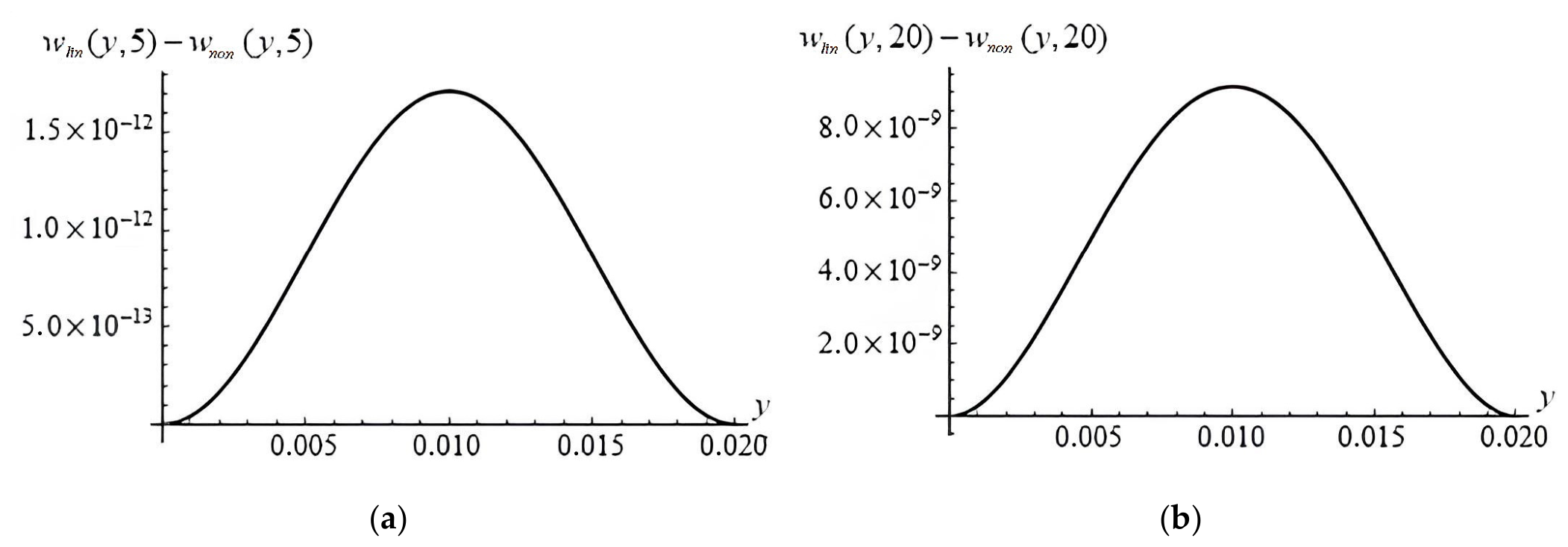
Figure 8 shows the calculations for $m=8$ at $t=5$ (Figure 8a) and $t=20$ (Figure 8b), where $w_{lin}(y,t), w_{non}(y,t)$ are the plate deformations obtained by solving the system of Equations (55) and (58), respectively.

Figure 8 shows the difference between the solutions of the linear and nonlinear models. As we can see from Figure 8, the effect of nonlinearity of the longitudinal force has an insignificant effect on the magnitude of the plate deflection, while the plate deflection decreases.

8. Conclusions

The paper studies the joint dynamics of the pressure sensor and the working medium in the pipeline on the basis of linear and nonlinear mathematical models that take into account the initial deformation of the elastic element and the transfer of heat flow through the pipeline with the working medium from the motor to the elastic element. The study of the elastic element dynamics is based on the application of the small parameter method, Galerkin method and numerical experiment in Mathematica 12.0. The case of rigid fixation of the elastic element ends is considered. The above approach can also be applied to pipelines with modified end geometry. A comparative analysis of the results obtained for the linear and nonlinear model is carried out.

References

1. Chehreghani, M.; Misra, A.K.; Paidoussis, M.P. Dynamics of a cantilevered pipe conveying fluid and partially subjected to a confined counter-current external axial flow of a different fluid. J. Sound Vib. 2024, 590, 118574. [Google Scholar] [CrossRef] [Scilit]
2. Shaaban, A.; Chehreghani, M.; Misra, A.K.; Paidoussis, M.P. Experiments on the dynamics of aspirating cantilevered pipes concurrently subjected to reverse external axial flow. J. Sound Vib. 2023, 561, 117817. [Google Scholar] [CrossRef] [Scilit]
3. Aulisa, E.; Ibragimov, A.; Kaya-Cekin, E.Y. Fluid structure interaction problem with changing thickness beam and slightly compressible fluid. Discret. Contin. Dyn. Syst. 2014, 7, 1133–1148. [Google Scholar] [CrossRef] [Scilit]
4. Faal, R.T.; Derakhshan, D. Flow-Induced Vibration of Pipeline on Elastic Support. Procedia Eng. 2011, 14, 2986–2993. [Google Scholar] [CrossRef] [Scilit]
5. Kheiri, M.; Paidoussis, M.P. Dynamics and stability of a flexible pinned-free cylinder in axial flow. J. Fluids Struct. 2015, 55, 204–217. [Google Scholar] [CrossRef] [Scilit]
6. Giacobbi, D.B.; Semler, C.; Paidoussis, M.P. Dynamics of pipes conveying fluid of axially varying density. J. Sound Vib. 2020, 473, 115202. [Google Scholar] [CrossRef] [Scilit]
7. Abdelbaki, A.R.; Paidoussis, M.P.; Misra, A.K. A nonlinear model for a hanging cantilevered pipe discharging fluid with a partially-confined external flow. Int. J. Non-Linear Mech. 2020, 118, 103290. [Google Scholar] [CrossRef] [Scilit]
8. Mogilevich, L.I.; Popova, E.V. Longitudinal waves in the walls of an annular channel filled with liquid and made of a material with fractional nonlinearity. Izv. Vyss. Uchebnykh Zaved. Prikl. Nelineynaya Din. 2023, 31, 365–376. [Google Scholar]
9. Blinkov, Y.A.; Blinkova, A.Y.; Evdokimova, E.V.; Mogilevich, L.I. Mathematical modeling of nonlinear waves in an elastic cylindrical shell surrounded by an elastic medium and containing a viscous incompressible liquid. Acoust. Phys. 2018, 64, 274–279. [Google Scholar] [CrossRef] [Scilit]
10. Mogilevich, L.I.; Popov, V.S.; Popova, A.A.; Christoforova, A.V.; Popova, E.V. Mathematical modeling of three-layer beam hydroelastic oscillations. Vibroeng. Procedia 2017, 12, 12–18. [Google Scholar] [CrossRef] [Scilit]
11. Mogilevich, L.I.; Popov, V.S.; Popova, A.A. Longitudinal and transverse oscillations of an elastically fixed wall of a wedge-shaped channel installed on a vibrating foundation. J. Mach. Manuf. Reliab. 2018, 47, 227–234. [Google Scholar] [CrossRef] [Scilit]
12. Velmisov, P.A.; Ankilov, A.V.; Semenova, E.P. Mathematical modeling of aeroelastic systems. In Applications of Mathematics in Engineering and Economics (AMEE’17); Pasheva, V., Popivanov, N., Venkov, G., Eds.; AIP Conference Proceedings 1910; AIP Publishing LLC: Melville, NY, USA, 2017; pp. 1–8. [Google Scholar] [CrossRef] [Scilit]
13. Velmisov, P.A.; Ankilov, A.V.; Pokladova, Y.V. Stability of solutions of initial-boundary value problems in aerohydroelasticity. In Applications of Mathematics in Engineering and Economics (AMEE’18); Pasheva, V., Popivanov, N., Venkov, G., Eds.; AIP Conference Proceedings 2048; AIP Publishing LLC: Melville, NY, USA, 2018; pp. 1–10. [Google Scholar] [CrossRef] [Scilit]
14. Velmisov, P.A.; Ankilov, A.V. Mathematical modeling of some aerohydroelastic systems. In Applications of Mathematics in Engineering and Economics (AMEE’21); AIP Conference Proceedings 2371; AIP Publishing LLC: Melville, NY, USA, 2021; p. 040009. [Google Scholar]
15. Velmisov, P.A.; Pokladova, Y.V. Mathematical modelling of the “pipeline–pressure sensor” system. J. Phys. Conf. Ser. 2019, 1353, 012085. [Google Scholar] [CrossRef] [Scilit]
16. Velmisov, P.A.; Tamarova, Y.A.; Pokladova, Y.V. Mathematical modelling of pressure monitoring systems in fluid and gaseous media. In Applications of Mathematics in Engineering and Economics (AMEE’20); AIP Conference Proceedings 2333; AIP Publishing LLC: Melville, NY, USA, 2021; p. 120004. [Google Scholar] [CrossRef] [Scilit]
17. Mihajlov, P.G.; Mokrov, E.A.; Mitrohin, S.V.; Sergeev, D.A. Features of metrological support for modern pressure pulsation sensors. News South. Fed. Univ. Tech. Sci. 2012, 130, 174–179. (In Russian) [Google Scholar]
18. Mikhailov, P.G.; Mokrov, E.A.; Sergeev, D.A.; Skotnikov, V.V.; Petrin, V.A.; Chernetsov, M.A. Sensitive elements of high-temperature pressure sensors. Materials and manufacturing technologies. Izv. SFedU. Eng. Sci. 2014, 153, 204–213. (In Russian) [Google Scholar]
19. Pirogov, S.P. Manometric Tubular Springs; Nedra: St. Petersburg, Russia, 2009. (In Russian) [Google Scholar]
20. Pirogov, S.P.; Cherentsov, D.A.; Chuba, A.Y.; Ustinov, N.N. Simulation of forced oscillations of pressure monitoring devices. Int. J. Eng. Trends Technol. 2022, 70, 32–36. [Google Scholar] [CrossRef] [Scilit]
21. Etkin, L.G. Vibration Frequency Sensors. Theory and Practice; Publishing house of MSTU N.E. Bauman: Moscow, Russia, 2004. (In Russian) [Google Scholar]
22. Belozubov, E.M.; Vasiliev, V.A.; Zapevalin, A.I.; Chernov, P.S. Design of elastic components of nano- and microelectromechanical systems. Meas. Tech. 2011, 54, 21–24. [Google Scholar] [CrossRef] [Scilit]
23. Dmitrienko, A.G.; Isakov, S.A.; Belozubov, E.M. Pressure sensors based on nano- and microelectromechanical systems for rocket and aviation technology. Sens. Syst. 2012, 160, 19–25. (In Russian) [Google Scholar]
24. Belozubov, E.M.; Mokrov, E.A.; Tikhomirov, D.V. Minimizing the error of thin-film strain-resistive pressure sensors under the influence of non-stationary temperature. Sens. Syst. 2004, 1, 26–29. (In Russian) [Google Scholar]
25. Stuchebnikov, V.; Vaskov, Y.; Savchenko, E. Special pressure sensors of the MIDA industrial group. Compon. Technol. 2021, 238, 12–15. (In Russian) [Google Scholar]
26. Kazaryan, A.A.; Groshev, G.P. Universal pressure transducer. Meas. Tech. 2008, 51, 269–275. [Google Scholar] [CrossRef] [Scilit]
27. Savchenko, E.G.; Stuchebnikov, V.M.; Ustinov, A.A. Features of the design of high-temperature strain gauge pressure transducers based on SNS structures. Instruments 2016, 189, 1–7. (In Russian) [Google Scholar]
Figure 1. Pipe with sensor.
Engproc 150 00129 g001
Figure 2. Initial approximation of plate deflection.
Engproc 150 00129 g002
Figure 3. Initial effect of the longitudinal force nonlinearity.
Engproc 150 00129 g003
Figure 4. Change in temperature of the working medium along the length of the pipeline: (a) at time points t = 3600 ; (b) at time points t = 36,000 .
Engproc 150 00129 g004
Figure 5. Temperature change in the working medium at the plate boundary.
Engproc 150 00129 g005
Figure 6. Deformation of the plate at times t = 5 (a) and t = 20 (b) for m = 8 .
Engproc 150 00129 g006
Figure 7. Deformation of the plate at the point y = 0.01 , t [ 0 , 5 ] (a) and t [ 0 , 20 ] (b), m = 8 .
Engproc 150 00129 g007
Figure 8. The difference in the plate deformation in models (8) and (9) at times t = 5 (a) and t = 20 (b) for m = 8 .
Engproc 150 00129 g008
Disclaimer/Publisher’s Note: The statements, opinions and data contained in all publications are solely those of the individual author(s) and contributor(s) and not of MDPI and/or the editor(s). MDPI and/or the editor(s) disclaim responsibility for any injury to people or property resulting from any ideas, methods, instructions or products referred to in the content.