State-Based Estimation of Future Mission Capability for Degrading Unmanned Aerial Vehicles ^†

Abstract

Reliability assessment in complex technical systems often involves capturing the interdependency between multiple subsystems and the gradual loss of their functional effectiveness. This challenge becomes particularly critical in the context of Unmanned Aerial Vehicles (UAVs), where sustained operational capability is essential for the safe execution of autonomous missions. This work presents a state-based methodology to estimate the future mission capability of UAVs subject to progressive component degradation. To generate a representative dataset, around 600 simulated flight missions for each of the 70 UAV fleet members are conducted, distinguished by randomly varying degradation profiles across multiple actuators. A hidden semi-Markov model (HSMM) is trained on this data to characterize the progressive reduction in system performance over time. To improve model tractability and generalization, raw flight data is first reduced to a concise set of performance-related parameters, from which critical sensor signals, such as roll, pitch, yaw, horizontal and vertical airspeeds, and current consumption, are estimated. The approach is evaluated in comparison to Decision Tree (DT) and XGBoost (XGB) models in a 5-fold cross-validation analysis. It enables the identification of system-wide dependencies between degradation patterns and mission-relevant behavior. By linking current operational states to the likelihood of meeting future performance requirements, it offers a quantitative basis for predictive reliability assessment. The best performance is achieved by an XGB model, whose mission capability estimation roughly doubles the number of conducted missions up to a failure by avoiding risky missions in comparison to unfiltered mission acceptance.

1. Introduction

The use of UAVs is increasing, as is their range of application [1]. Their operation will require compliance with regulations, which especially focus on an operational risk assessment and ensuring a target level of safety [2]. New operating concepts for Unmanned Air Traffic Management (UTM) therefore account for responsible risk management approaches [3]. For autonomous UTM participants, contingency management systems are proposed, which shall determine the mission procedure, considering the safety of continued operations [4,5]. In the context of such decision-making, assessing the UAV’s condition through an integrated vehicle health management system becomes essential. In a survey among UAV operators by Osborne et al. [6], advanced warnings for battery faults and electrical or mechanical failures are a top priority to those.

The influence of UAV subsystems on the mission risk can be analyzed through a Failure Mode and Effect Analysis (FMEA). Shafiee et al. [7] describe a fault tree analysis and FMEA for UAV failures during inspection of offshore wind turbines. In a similar FMEA by Wang et al. [8], an analysis of the UAV by means of a finite element simulation is incorporated. Both analyses assign the highest risk priority numbers to battery and motor malfunctions, while further potential failure sources are the flight controller, communication and sensor modules and the UAV structure. The highest concern in terms of battery usage is falling below a sufficient state of charge [7,8]. Typical degradation effects on UAV batteries result in a decreased maximum charge capacity with an increasing number of charge cycles [9]. For Brushless Direct Current (BLDC) motors, which are propelling the UAV blades, dominant failure modes are bearing degradation, electrical failures and permanent magnet failures [10,11]. If there are UAV control surfaces, actuated by servo motors, those will also degrade over time [12,13] and may become less accurate in achieving the target angles [12]. In addition to the condition of UAV subsystems, weather conditions can have a huge influence on flight stability [14]. Both the modelling of wind in urban environments [15] and of wind influences on UAV behavior [16] highlight the complexity of effectively adapting to wind conditions.

Analyzing the complete UAV’s capability to conduct further missions can be achieved with model-based fault detection approaches, which compare observed and expected sensor data [17]. Another option is stochastic modelling; for instance, Ancel et al. [18] propose the utilization of Bayesian Belief Networks to represent the interconnection of real-time component failure indicators. The potential of data-driven methods to predict the future availability of safety-critical components and their impact on the system behavior is demonstrated in [19]. In that study, the components of a multicopter electric powertrain are monitored for their performance, and their future behavior is predicted using a Kalman filter. This approach is applied to the complete system, which reaches its performance limit significantly earlier than its components. Rodrigues [20] also determines a performance indicator for the overall system based on the states of its components. The evolution of component states is modeled using particle filters, and their interaction at the system level is represented via a system architecture function. Heier [21] represents the impact of partial failures on individual subsystems using logical fault tree connections and then predicts the probability of possible failure combinations of the subsystems at the system level.

While existing approaches for UAV reliability assessment provide valuable insights through failure mode analysis and component-level prognostics, they often lack an integrated, data-driven framework that captures system-wide interdependencies and translates component degradation into mission-level capability predictions. The current methods either rely on static fault models that may not reflect progressive degradation dynamics or focus on individual component prognostics without accounting for how degradation across multiple subsystems affects overall mission performance. To bridge this gap, this work proposes a state-based approach that directly models the relationship between progressive component degradation and mission capability through hidden semi-Markov modeling.

2. Flight Simulation and Mission Capability Estimation Approach

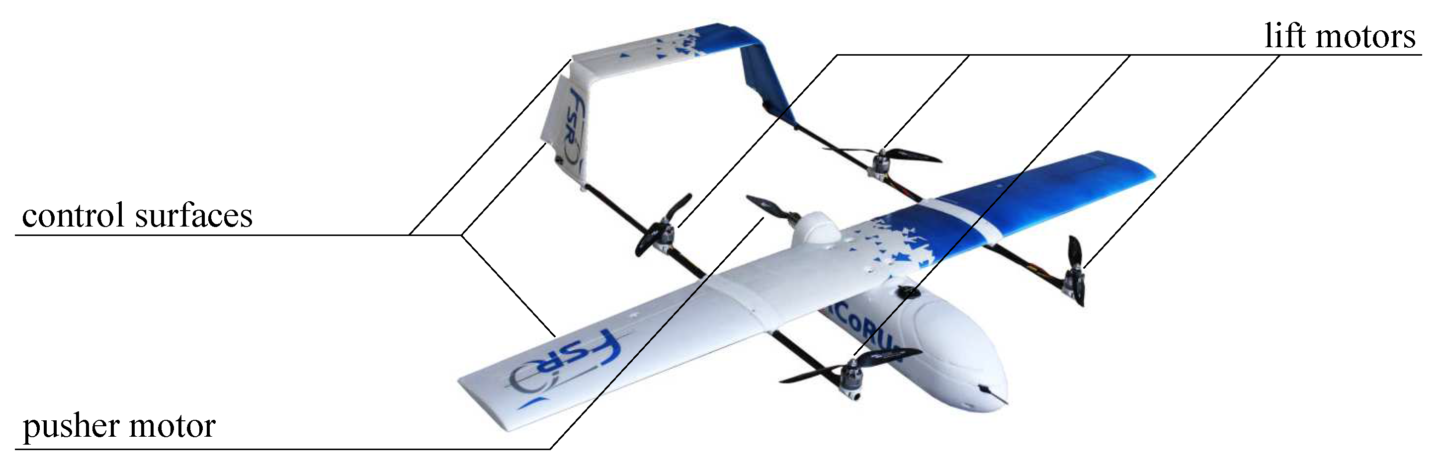
In this work, a flight simulation model is utilized to analyze the influence of a performance reduction of several UAV actuators due to degradation on the flight stability. The model represents a hybrid UAV configuration capable of both fixed-wing flight and multicopter flight, which is depicted in Figure 1. A comprehensive description of the UAV is provided in [22] and its aerodynamic properties are discussed in [23]. The flight model in these works is based on the formulation of UAV flight equations developed during the creation of combined physics-based and data-driven flight state estimation models, which are described in [24]. With the flight mechanics and actuation force model, the physical response of the UAV to the flight controller, a locally executed ArduPilot instance as described in [25], is represented. The database of simulated flights is utilized to estimate the capacity of degraded UAVs to conduct further missions.

Figure 1. Hybrid UAV “SciHunter” with fixed-wing and hover flight capability.

2.1. Simulated Flight Behavior

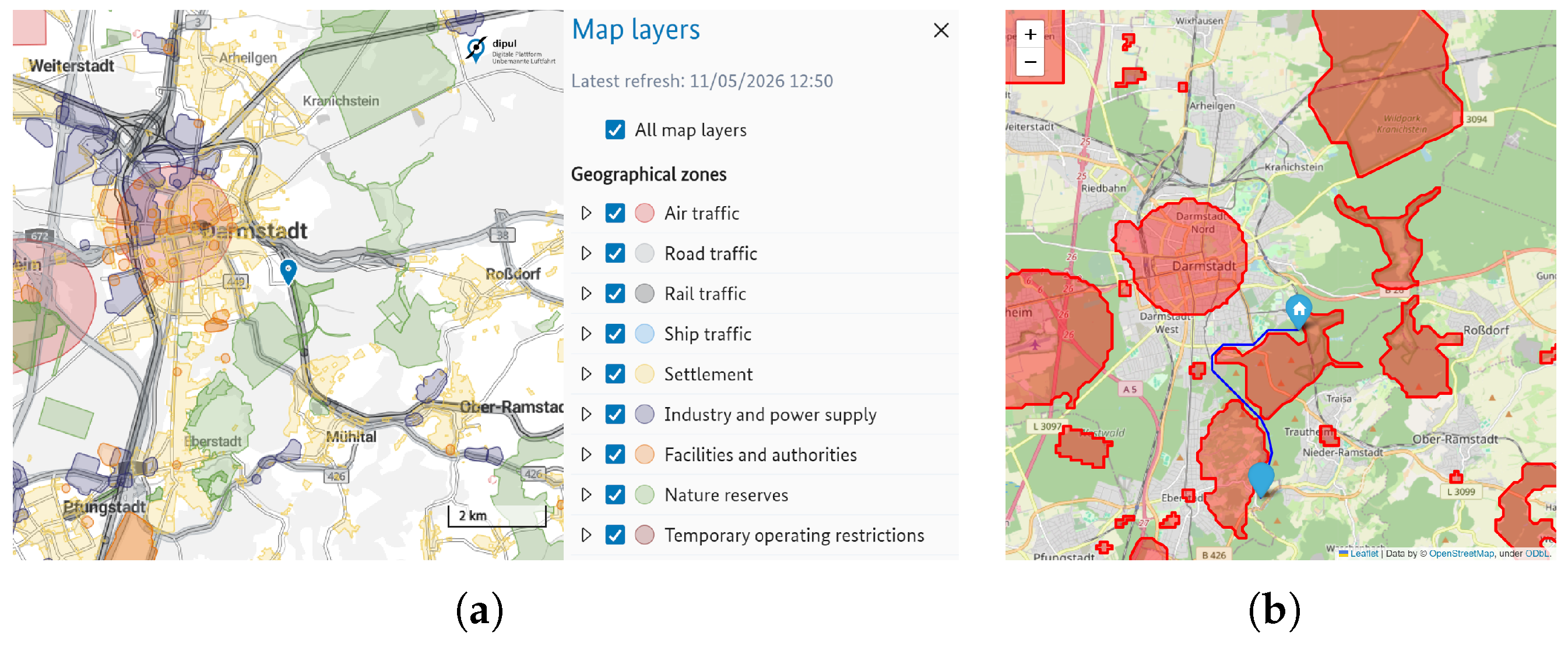
The simulation environment is designed to replicate realistic and variable mission profiles based on transport or reconnaissance missions. The simulated mission profiles include outbound and return flights between a fixed home waypoint and randomly generated destination points with a distance of at least 3 km and a maximum of 5 km, whereby intermediate waypoints are defined through route planning to avoid restricted airspace. An exemplary mission and the considered restricted airspace based on the Map Tool of the Digital Platform for Unmanned Aviation [26] are displayed in Figure 2. Furthermore, a random wind profile is generated for each mission, which is incorporated as a repeatable pattern of slightly varying wind speeds and directions. Each mission consists of the flight phases of multicopter mode during take-off and landing, fixed-wing flight along the route to the target, and two transition phases between multicopter and fixed-wing flight.

Figure 2. (a) Airspace Map Tool provided by the Digital Platform of Unmanned Aviation [26]. (b) Exemplary mission path planning.

For 70 simulated UAVs, the increasing degradation of individual UAV components is modeled with varying degradation rates. The goal of the simulations is to identify missions that can no longer be conducted by the simulated UAV. The simulated degradation of the UAV subsystems includes the BLDC motors, the servo motors, and the battery. The base values for the degradation rates are chosen in such a way that first failures caused by a single degrading system without wind disturbances occur after approximately 1000 missions. This conservative choice is intentional to enable the observation of error-prone missions within a feasible range of simulation effort and data imbalance. Individual degradation rates are sampled from a normal distribution with a standard deviation of 0.2, with 1–3 randomly selected rates retained as dominant modes, while the remaining rates are scaled to 0.05–0.33 of their sampled value to create heterogeneous degradation patterns across the UAV fleet. Degradation rates increase quadratically with the mission index to approximate accelerating degradation patterns similar to empirical observations, for example, in battery aging. The quadratic coefficient is randomly varied to produce increased degradation rates at mission 1000 with ratios to mission 1 ranging from 1.4 to 2.8, while an adaptive bias factor ensures a consistent mean degradation rate across all trajectories.

For the BLDC motors, a decrease in efficiency over the course of operation is assumed, similar to the approach in [19], where degradation of UAV motors is simulated through a decline in rotational speed, or the observation in [27] of increasing thrust reductions with increasing propeller degradation of UAV driving trains. The mechanical power within the simulation is derived in accordance with the motor’s pwm input signal and scaled with a health efficiency value, ${\eta }_h$, which is reduced by $10\%$ after 1000 missions at the base failure rate. The servo motors are affected by random deviations between the control signal and the resulting control surface angle, with the variance increasing with each actuation, as observed in [12]. In the simulation, a random variation in the pwm signals specifying the target servo angles is included, distorting their values with a standard derivation of ${\displaystyle \frac{4}{3}}$ of the original input scale after 1000 missions. The battery exhibits a decreasing maximum capacity with each charge cycle due to the degradation mechanisms described in [9], which result in a loss of active anode or cathode material or lithium inventory. The maximum state of charge of the battery is reduced by $20\%$ after 1000 missions at the base failure rate.

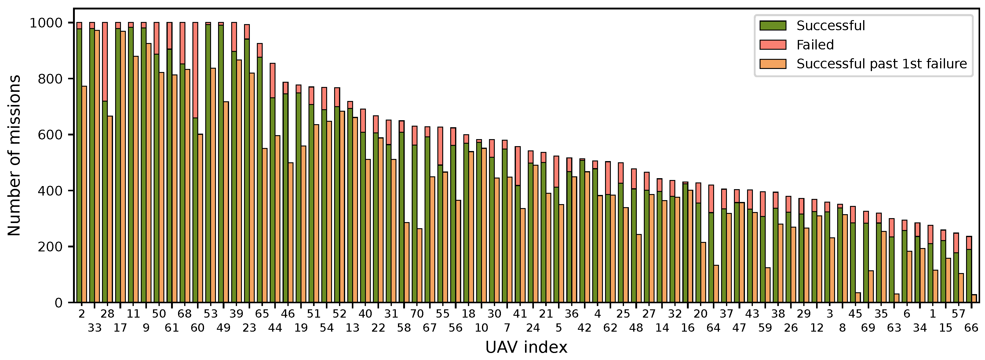
Criteria for mission success are a controlled landing at the target destination and remaining within a 180 m wide horizontal mission corridor throughout the flight. The number of simulated missions per UAV is shown in Figure 3. For each UAV, either 1000 simulated missions are conducted or the simulation is not continued after 10 consecutive failed missions. A second bar for each UAV displays how many successful missions are still simulated after a first failed mission. It indicates that the mission failures are not solely dependent on UAV subsystem degradation but are also influenced by environmental conditions, with many UAVs experiencing first failures rather early in their lifetime and being able to conduct many successful missions again after those.

Figure 3. Number of conducted missions for each UAV, sorted by total amount of missions.

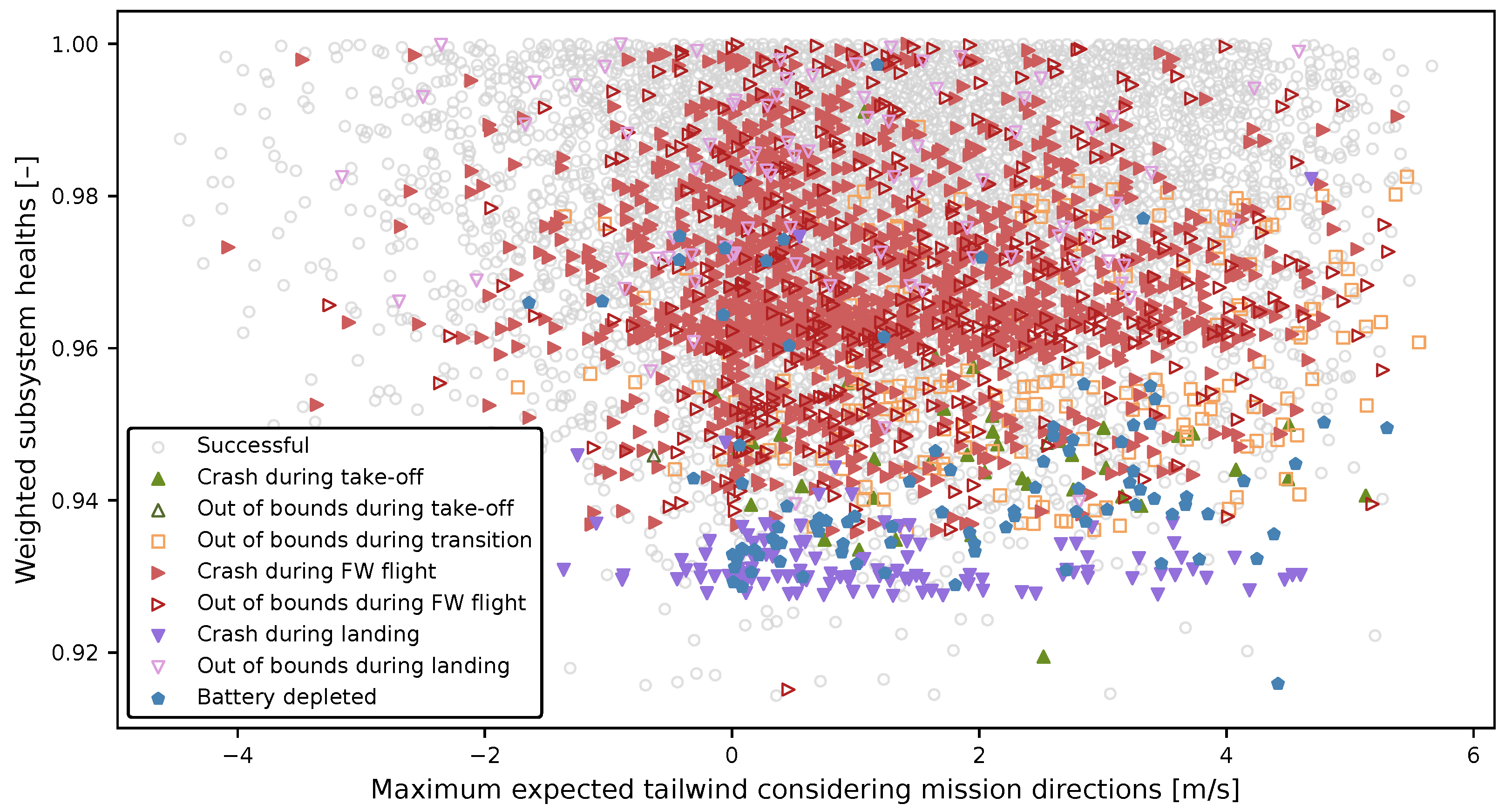
The influence of degradation and environmental conditions on the mission success is also visualized in Figure 4. It illustrates that missions with high health values and favorable wind conditions are rather likely to be successful, while failures become more frequent for adverse conditions. The expected environmental conditions of future missions must therefore necessarily be taken into account when predicting the future mission capability. It also becomes apparent that there are a multitude of factors that influence the success of a mission, and that even missions with seemingly very similar starting conditions can yield different results.

Figure 4. Mission outcome depending on health and wind conditions within the simulation database. Missions with headwind throughout the route are less prone to failures compared to missions with tailwind segments. With lower subsystem health values, more failures occur. The amount of visible failures also depends on the amount of available data points, with the highest density for high health and small wind values. The weighted subsystem health is calculated as the weighted sum of average subsystem health values, minimum subsystem health value and imbalance in lift motor health values. Certain failures, like crashes during the landing, only appear if multiple subsystems are noticeably degraded.

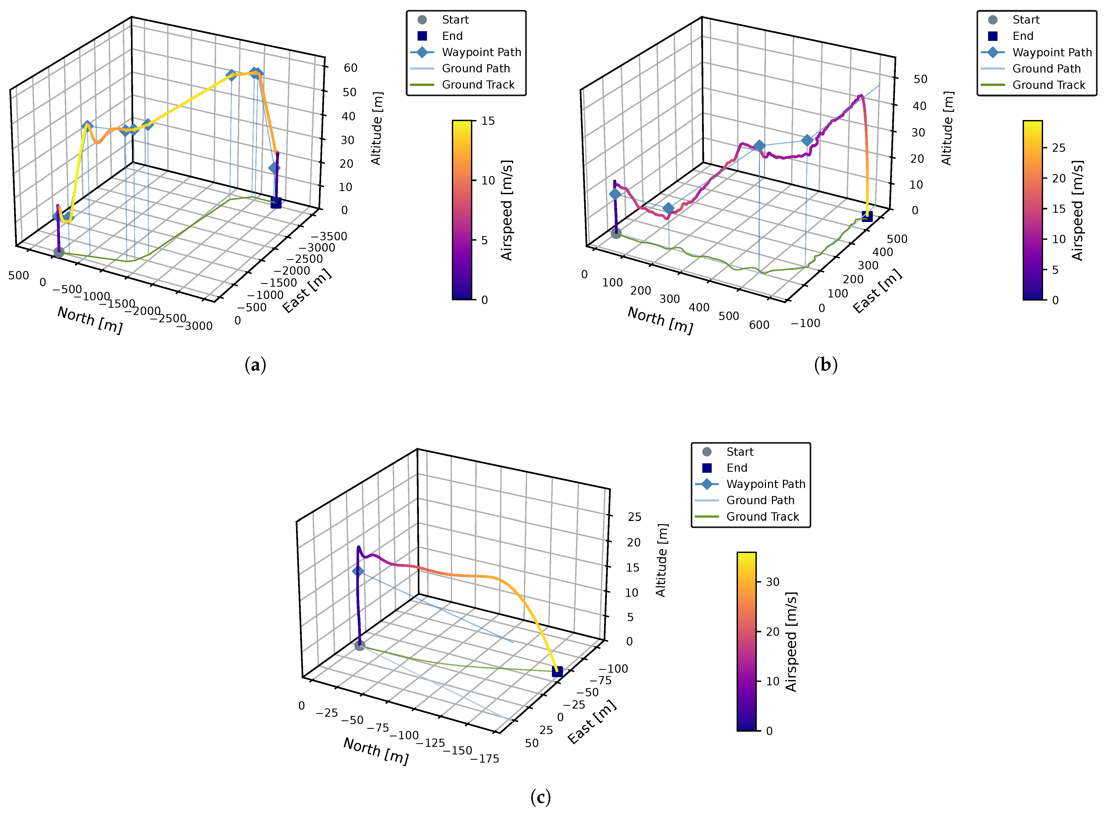
Failed missions particularly occur during fixed-wing flight and the transition to fixed-wing flight. During fixed-wing flight, limited functionality of the pusher motor or the control surfaces can result, depending on wind conditions, in insufficient attitude and velocity control to generate the required lift, which can lead to UAV crashes. Progressive degradation of the lift motors affects the hover phase stability, with tilted flight attitudes after affected hover phases also significantly complicating the subsequent transition. The resulting failures are depicted in Figure 5 for both a rotation during fixed-wing flight with a resulting loss of lift and an unstable transition due to a tilted hover position resulting in increasing deviation from the intended path.

Figure 5. (a) Flight path of a successful mission. (b) Loss of lift during fixed-wing flight. (c) Mission corridor violation during the transition.

2.2. Flight Data Processing

The raw simulation data is recorded at a frequency of 100 Hz and encompasses 120 channels, including inertial measurement unit values, attitude and velocity estimations, aerodynamic coefficients, motor currents, rotational speeds, and wind estimations in multiple spatial directions. Additionally, nine health channels monitor the degradation state of the propulsion system (pusher and four lift motors), control surfaces (aileron, elevator, rudder), and the battery. A typical mission scenario spans a distance of 3 km to 5 km with durations ranging between 300 s and 1000 s.

The flight data is divided into distinct flight segments based on the active flight mode of the ArduPilot flight controller. The defined ten flight modes capture the varied dynamic behaviors of a hybrid UAV: vertical take-off (0), transition to fixed-wing (1), acceleration (2), climb to cruise (3), cruise (4), descent (5), transition to hover (6), hover (7), multicopter descent (8), and precise landing (9). Notably, the cruise mode is subdivided into multiple segments for each waypoint leg. While the initial sub-segment involves no heading change, subsequent segments encapsulate the required turn maneuvers.

For each identified segment, statistical features are derived from six critical sensor signals that possess a strong physical correlation with performance and degradation. These signals are roll angle ($\varphi$), pitch angle ($\theta$), waypoint-relative yaw angle ($\Delta \psi$), horizontal airspeed ($v_h$), vertical airspeed ($v_v$), and total current consumption ($I_{\mathrm{total}}$). Ten statistical metrics are extracted per signal per segment to summarize both the main segment behavior and the occurrences of extreme deviations, resulting in 60 feature representations for the sensor data. Their formal definitions are detailed in Table 1. An additional list of disregarded features is defined on an analytical basis, which may exclude certain sensor information for certain flight modes (like horizontal speed information in purely vertical flight segments) or specific features for certain sensors (e.g., whether the occurrence of extreme deviations is described in regard to the flight time, the origin or the target distance). The features are augmented by mission-specific predictors like the wind profile, separated into along-track ($w_{\Vert }$), cross-track ($w_{\perp }$), and vertical ($w_v$) mean value and standard deviation, and geometric features such as turn angle ($\Delta {\psi }_{\mathrm{turn}}$), horizontal distance ($d_h$), and vertical distance ($d_v$). As the waypoints for a mission are predefined, the required geometries are known in advance, and the wind behavior can be robustly predicted or estimated for each upcoming segment.

Table 1. Extracted statistical metrics per segment and sensor signal x.

Metric Name	Description	Formula/Definition
Mean ($\mu$)	Main behavior of the signal.	${\mu }_x={\displaystyle \frac{1}{N}}{\sum }_{i=1}^N{x}_i$
Standard Deviation ($\sigma$)	Signal variation within the segment.	${\sigma }_x=\sqrt{{\displaystyle \frac{1}{N}}{\sum }_{i=1}^N{(x_i-{\mu }_x)}^2}$
Absolute Maximum ($\mid x-{\mu }_x{\mid }_{max}$)	Peak absolute magnitude observed.	$max(\mid x-{\mu }_x\mid )$
Max Index (${\mid x\mid }_{max}\mathrm{idx}$)	Chronological index of peak magnitude.	${\mathrm{argmax}}_i(\mid x-{\mu }_x\mid )$
High-Dev. Start/End Index	Chronological start and end index of most prominent deviation region above the 95% confidence interval.	Indexes $i_s,i_e$ where $\mid x_i-{\mu }_x\mid > 1.96·\sigma$
High-Dev. Distance to Origin	Spatial displacement from waypoint segment start during high deviation event.	$d_{\mathrm{ori}}\left(i_s\right)$, $d_{\mathrm{ori}}\left(i_e\right)$
High-Dev. Distance to Target	Spatial displacement to target waypoint during high deviation.	$d_{\mathrm{tgt}}\left(i_s\right)$, $d_{\mathrm{tgt}}\left(i_e\right)$

To isolate genuine degradation effects from regular environmental responses, the derived features undergo a selection and environmental detrending process. Features exhibiting near-zero variance due to inactive signals or high noise components are excluded. To counteract the influence of varying weather conditions and mission geometries on flight stability, a multiple linear regression model estimates predictable deviations based on wind estimators and geometric predictors:

$$y_s={\beta }_0+\sum _p{\beta }_p·x_{p,s}+{\alpha }_u·m$$

(1)

Here, the measured target characteristic $y_s$ for segment s is estimated through a baseline offset ${\beta }_0$, the impact of the environmental predictors $x_{p,s}$ scaled by their coefficients ${\beta }_p$, and a degradation-related temporal drift term modeled as a linear evolution ${\alpha }_u$, independent for each UAV, based on the progressive mission index m of the current UAV. After predicting the expected behavior governed by the environmental conditions, the residuals represent the detrended, environment-independent variations which are subsequently standardized over the UAV’s lifecycle.

Since a full mission comprises multiple segments spread across the ten flight modes, the feature scope must be consolidated. Principal Component Analysis (PCA) maps the high-dimensional segment features into j condensed mission variables, facilitating critical dimensional reduction. In cases where the flight mode occurs multiple times along distinct waypoint legs (e.g., cruise sections), the median of the feature statistics across these segments is selected to represent the overarching condition within the given mode. The standardizer and PCA strictly rely on data from successful missions to establish an uncorrupted baseline of generic variance. The optimal number of condensed features j constitutes a hyperparameter dynamically tuned during the subsequent mission capability modeling, with typical optimization bounds aiming between 2 and 10 resulting PCA features.

2.3. Mission Capability Estimation

Assessing the reliability of complex technical systems generally requires capturing the dynamic interdependencies among degrading components. While combinatorial coherent models, such as fault trees, are frequently employed, they are fundamentally restricted in their descriptive depth. State-space approaches, such as Markov models, offer significantly greater modeling power by effectively representing interacting subsystems, parallel processes, and cascading dependencies during system degradation [28]. However, classical Hidden Markov Models (HMMs) rely on the inherently limiting assumption of exponentially distributed state durations [29]. To address this operational constraint, Hidden Semi Markov Models (HSMMs) have successfully been integrated into reliability engineering, allowing for arbitrary sojourn time distributions that more realistically represent progressive physical wear [30,31]. Extending this framework, Multibranch Hidden Semi Markov Models (MB-HSMMs) accommodate the fact that real-world deterioration does not inherently trace a singular unified sequence. Instead, by introducing multiple independent state-transition branches, a MB-HSMM can simultaneously represent distinct parallel failure pathways and dynamic response models [32].

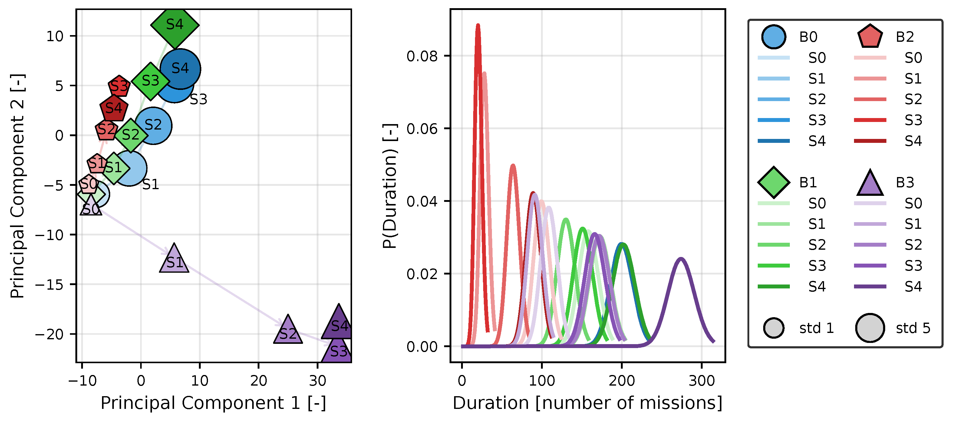
In this work, a MB-HSMM integrates the aggregated sequence of condensed mission features (the extracted j PCA components) to stochastically map the progressive UAV condition, tracing the trajectory from a fully capable operational baseline through intermediate performance degradations down to potential critical failure states, similarly to that observed in [33]. The full topological architecture, encompassing the assigned number of distinct degradation branches (considered between 3 and 6), the discrete health states per branch (considered between 4 and 8), and the required constraints on observation sequence lengths, is dynamically structured as system hyperparameters. To model a monotonic degradation behaviour, the probabilities of state transitions are defined in such a way that they only allow for a transition to the next higher state. The probability of remaining in a state with a residence duration is modelled using Poisson distributions, whereby the minimum and maximum residence durations under consideration are determined such that the distribution covers between $50\%$ and $99\%$ of the expected durations, depending on the variation in the duration-confidence hyperparameter. Training is facilitated by an iterative viterbi prediction of the expected state sequences from the observation sequences of each branch, with increasing refinement of the expected observation and residence duration values per state, followed by an update and reallocation of sequences to the branches that best represent them. Exemplary training results of one MB-HSMM are visualized in Figure 6. To guarantee robust out-of-fold generalization, model training and evaluation are conducted via a comprehensive 5-fold cross-validation scheme. Across the database of 70 simulated UAVs, each data split operates independently by allocating 56 UAVs for training and reserving the remaining 14 UAVs strictly for validation testing. This work focuses exclusively on discussing the results achieved by the strongest models in the context of hyperparameter optimization, thereby preserving scope for further investigation of these models using unseen test data.

Figure 6. Progression mapping of the primary condensed mission variables (PC1 versus PC2) isolating distinctly identified degradation pathways and states across the trained MB-HSMM branches.

The risk evaluation strategy leverages the trained MB-HSMM framework to anticipate conditional success probabilities for future missions, given a recorded system-level operational history. For an ongoing sequence up to the prevailing timestep, the most probable underlying stochastic state and active degradation branch are deduced. Recognizing the profound operational influence of aerodynamic variances on heavily degraded systems, a k-Nearest Neighbor (KNN) context search evaluates past missions mapped to identical states and corresponding branches. Similarity is structurally weighted utilizing Euclidean distances across 10 inherently scaled environmental and geometric constraints: five parameters describing wind conditions in general (maximum and minimum tailwind and maximum absolute sidewind relative to the planned flightpath, mean and standard deviation of the wind speed), three constraints specifically addressing take-off wind configurations (mean takeoff headwind, sidewind and wind angle), and two structural parameters defining the planned mission geometry (cumulative mission distance and cumulative size of turn angles). The resulting empirical survival probability derived from the nearest N contextual neighbors determines the expected overall success ratio.

As a comparison of the predictive capabilities and potential advantages of the MB-HSMM architecture, standardized machine learning benchmarks are examined on an identical cross-validation structure. A standard DT classifier provides a transparent, threshold-based machine learning baseline capable of explicit operational rule extraction [34]. Furthermore, XGB serves as a sophisticated, massively scalable tree-boosting alternative—a framework proven capable of tracking interconnected, non-linear dependencies across heavily structured tabular reliability diagnostics [35]. As both methods are better suited for high-dimensional input data in comparison with the MB-HSMM approach, their training data consists of the segment features’ values of the last successful mission rescaled to the predicted missions’ expected wind conditions with the corresponding detrending coefficients and environmental and health description values of the missions. Two rudimentary analytical baselines, establishing a static operational life-limit on the count of allowed generic missions, alongside a naive random-selection boundary, provide completely unweighted metrics.

All associative architectural parameters, ranging from the sequence observation spans natively deployed within the MB-HSMM and the number of KNN evaluation neighbors k, directly to the regularization terms and maximal depth limits imposed on the comparative tree mechanisms, undergo an iterative optimization utilizing the define-by-run Optuna framework [36]. By flexibly adjusting the acceptable bounding limit for the predicted mission success ratio, diagnostic precision–recall curves are generated across the out-of-fold validation trials. These continuous bounding limits visually map the fundamental operational trade-off tightly intertwined within data-driven asset diagnostics: balancing the necessity to maximize UAV utilization and operational lifetime against stringently restricting the incidence rate of unrecoverable in-flight failures.

3. Results and Discussion

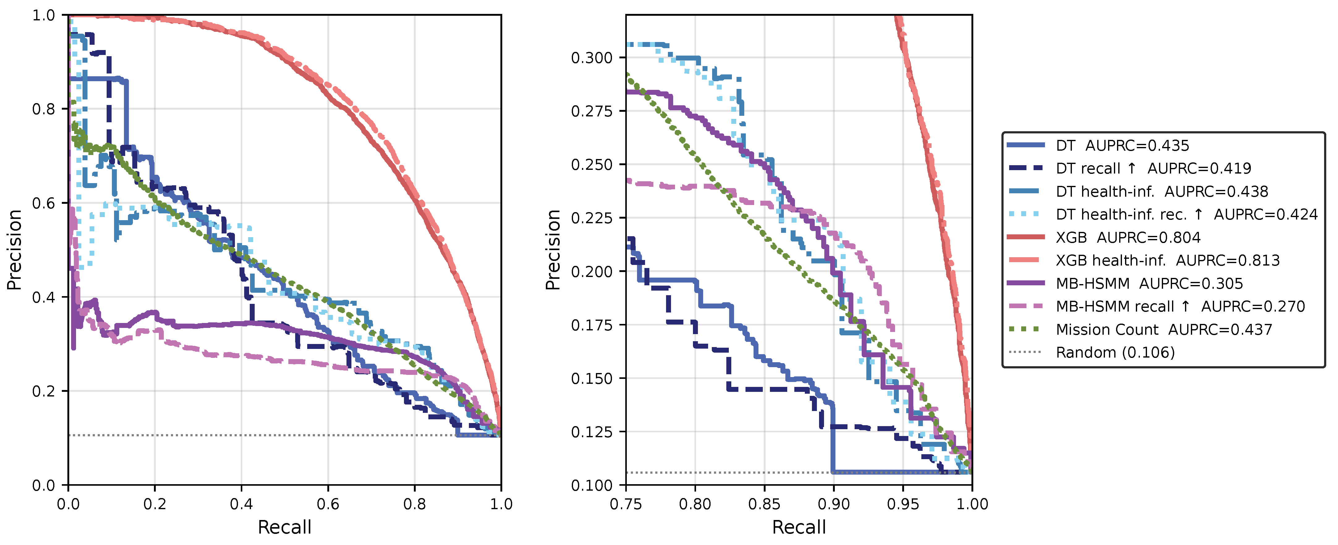
In Figure 7, precision–recall curves for the assessed predictive models across the cross-validation test folds are plotted. XGB demonstrates superior global performance both with and without access to the subsystem health values, which are not considered by the MB-HSMMs. The strong XGB performance is contributed to a high ability of its hierarchical architctecture to capture nuanced interactions between subsystems and mission profiles. However, the rather low achievable precision values indicate the remaining aleatoric uncertainty inherent in this deliberately challenging operating environment. Both the DT and XGB perform slightly better in overall Area Under Curve (AUC) with access to the health information features. The difference is more noticeable for DT models, which reach lower precision values for high recall values without subsystem health information. The comparatively low benefit of further health information could be caused by the high interdependence of the subsystems and the high observability of the effects of subsystem degradation on the system’s behaviour. Both the DT and MB-HSMM utilize an additional hyperparameter optimization with weighted AUC values to prioritize high-recall regions. For the XGB, both objectives lead to nearly identical precision–recall curves and only the configuration with maximized AUC is plotted. The DT classifier exceeds the MB-HSMM and, in its best configuration, the static mission limit in overall AUC, but especially outperforms them in low-recall regions of limited practical value. In those regions, uncertain mission outcomes for the MB-HSMM seem to limit their capability distinction ability, while a deterministic threshold allows for higher precision by simply attempting a higher amount of mission conductions. The MB-HSMM yields superior precision in the operationally critical high-recall boundaries compared to the mission number baseline and DT approach.

Figure 7. Precision–recall curves of the mission capability estimation models, with detailed visualization of high-recall region on the right.

Table 2 provides a comparison of fleet utilization capacity based on the quantity of successful test flights safely conducted before a first in-flight failure occurs. Only missions labeled as non-critical by the individual models are executed. Two threshold selection methods for criticality labeling are compared: one yielding an optimal F1-score, and one allowing for the most conducted missions up to a first failure within the test folds. Selecting valid operational profiles utilizing the XGB risk assessment effectively doubles the total operational volume achieved by the UAVs compared to a baseline strategy that continuously conducts missions without safety estimations and that would allow for a total of 6428 missions. The other models still allow for more conducted missions compared to an absence of safety estimation, but with a less significant increase. The improvement is also noticeably smaller when the F1-score-optimized threshold is utilized. Therefore, the optimal threshold should be tested in the future using separate flight simulation data outside the cross-validation set.

Table 2. Recall–precision combination influence on feasible missions. Precision, recall and F1-score are calculated on all out-of-fold data points, and successes counted up to first unpredicted failure for each out-of-fold UAV.

Model	F1-Optimal Advisory Until 1st Failure				Maximize Successes Until 1st Failure
	Precision	Recall	F1	#Success	Precision	Recall	F1	#Success
DT	0.435	0.492	0.462	6802	0.403	0.519	0.453	6840
DT optimized for high recall	0.531	0.379	0.442	6921	0.495	0.381	0.431	6921
DT health-informed	0.387	0.671	0.491	6744	0.365	0.688	0.477	6744
DT health-inf., opt. for high recall	0.547	0.418	0.474	6670	0.373	0.585	0.455	6746
XGB	0.758	0.681	0.717	8027	0.376	0.927	0.535	14,020
XGB health-informed	0.770	0.699	0.733	7098	0.308	0.951	0.465	12,463
MB-HSMM	0.314	0.779	0.415	6334	0.160	0.935	0.264	7836
MB-HSMM opt. for high recall	0.239	0.817	0.370	6543	0.166	0.947	0.282	7039

4. Conclusions and Further Work

This work presents a comprehensive risk evaluation pipeline for degrading UAVs, utilizing simulated telemetry and environmental data to dynamically estimate future mission capability. The assessment models the threshold between progressive component deterioration and operational survival by transforming complex flight behavior into condensed representations and employing techniques ranging from MB-HSMM infused with KNN contextual filtering to advanced tree-boosting architectures. The results show that integrating dynamic environmental predictors alongside structural degradation metrics significantly improves predictive reliability. The XGB framework doubles fleet utilization while maintaining a strict barrier against unrecoverable mid-flight failures.

Future research will investigate the direct inclusion of a selected subset of high-relevance physical features, as identified by the XGB model, into the MB-HSMM structure to test their efficacy compared to the present PCA transformation. Furthermore, the resilience of the combined approach will be studied by introducing varying data imputation and failed mission consideration strategies, alongside analyzing the complete pipeline’s sensitivity to artificially reduced sensor measurement quality and degradation-state noise. Ultimately, the methodologies established herein provide a robust foundation for active in-flight analysis. Diagnostic forecasting of expected sensor value behavior during unfolding mission segments can be explored to establish an anomaly detection layer and explore the achievable warning time between identifiable deviations from expected flight behavior and mission failure.

References

1. Mohsan, S.A.H.; Khan, M.A.; Noor, F.; Ullah, I.; Alsharif, M.H. Towards the Unmanned Aerial Vehicles (UAVs): A Comprehensive Review. Drones 2022, 6, 147. [Google Scholar] [CrossRef] [Scilit]
2. European Commission On the Rules and Procedures for the Operation of Unmanned Aircraft: 2019/947, 2019. Available online: http://data.europa.eu/eli/reg_impl/2019/947/oj (accessed on 28 July 2026).
3. Balakrishnan, K.; Polastre, J.; Mooberry, J.; Golding, R.; Sachs, P. Blueprint for the Sky: The Roadmap for the Safe Integration of Autonomous Aircraft; Technical Report; Airbus UTM: San Francisco, CA, USA, 2018. [Google Scholar]
4. Baculi, J.E.; Ippolito, C.A. Onboard Decision-Making for Nominal and Contingency sUAS Flight. In AIAA Scitech 2019 Forum; American Institute of Aeronautics and Astronautics: Reston, VA, USA, 2019. [Google Scholar] [CrossRef] [Scilit]
5. Eduardo, H.; Schmidt, J.R. Concept and Requirements for an Integrated Contingency Management Framework in UAS Missions. In 2021 IEEE Aerospace Conference (50100); IEEE: New York, NY, USA, 2021; pp. 1–17. [Google Scholar] [CrossRef] [Scilit]
6. Osborne, M.; Lantair, J.; Shafiq, Z.; Zhao, X.; Robu, V.; Flynn, D.; Perry, J. UAS Operators Safety and Reliability Survey: Emerging Technologies towards the Certification of Autonomous UAS. In 2019 4th International Conference on System Reliability and Safety (ICSRS); IEEE: New York, NY, USA, 2019; pp. 203–212. [Google Scholar] [CrossRef] [Scilit]
7. Shafiee, M.; Zhou, Z.; Mei, L.; Dinmohammadi, F.; Karama, J.; Flynn, D. Unmanned Aerial Drones for Inspection of Offshore Wind Turbines: A Mission-Critical Failure Analysis. Robotics 2021, 10, 26. [Google Scholar] [CrossRef] [Scilit]
8. Wang, B.; Ng, P.H.; Elhadidi, B.M.N.A.K.; Ang, H.S.; Moon, S.K. Failure Analysis and Finite Element Simulation for Structural Systems in an Unmanned Aerial Vehicle. In 2019 16th International Conference on Ubiquitous Robots (UR); IEEE: New York, NY, USA, 2019; pp. 636–640. [Google Scholar] [CrossRef] [Scilit]
9. Birkl, C.R.; Roberts, M.R.; McTurk, E.; Bruce, P.G.; Howey, D.A. Degradation Diagnostics for Lithium Ion Cells. J. Power Sources 2017, 341, 373–386. [Google Scholar] [CrossRef] [Scilit]
10. Kudelina, K.; Asad, B.; Vaimann, T.; Rassolkin, A.; Kallaste, A.; Lukichev, D.V. Main Faults and Diagnostic Possibilities of BLDC Motors. In 2020 27th International Workshop on Electric Drives: MPEI Department of Electric Drives 90th Anniversary (IWED); IEEE: New York, NY, USA, 2020; pp. 1–6. [Google Scholar] [CrossRef] [Scilit]
11. Weigert, M. Approach to Condition Monitoring of BLDC Motors with Experimentally Validated Simulation Data. PHM Soc. Eur. Conf. 2022, 7, 521–529. [Google Scholar] [CrossRef] [Scilit]
12. ElSaid, A.; Adjekum, D.; Nordlie, J.; Jamiy, F.E. A Test-Bed For Measuring UAS Servo Reliability. Aerospace 2019, 6, 96. [Google Scholar] [CrossRef] [Scilit]
13. Sarson-Lawrence, J.; Sabatini, R.; Clothier, R.; Gardi, A. Experimental Determination of Low-Cost Servomotor Reliability for Small Unmanned Aircraft Applications. Appl. Mech. Mater. 2014, 629, 202–207. [Google Scholar] [CrossRef] [Scilit]
14. Gao, M.; Hugenholtz, C.H.; Fox, T.A.; Kucharczyk, M.; Barchyn, T.E.; Nesbit, P.R. Weather Constraints on Global Drone Flyability. Sci. Rep. 2021, 11, 12092. [Google Scholar] [CrossRef] [Scilit] [PubMed]
15. Büddefeld, M.C. Hybrid Model for Downscaling Wind Information for Unmanned Aerial Systems. Ph.D. Thesis, Technische Universität Darmstadt, Darmstadt, Germany, 2025. [Google Scholar] [CrossRef]
16. Wang, B.H.; Wang, D.B.; Ali, Z.A.; Ting Ting, B.; Wang, H. An Overview of Various Kinds of Wind Effects on Unmanned Aerial Vehicle. Meas. Control 2019, 52, 731–739. [Google Scholar] [CrossRef] [Scilit]
17. Schumann, J.; Mahadevan, N.; Sweet, A.; Bajwa, A.R.; Lowry, M.; Karsai, G. Model-Based System Health Management and Contingency Planning for Autonomous UAS. In AIAA Scitech 2019 Forum; American Institute of Aeronautics and Astronautics: Reston, VA, USA, 2019. [Google Scholar] [CrossRef] [Scilit]
18. Ancel, E.; Capristan, F.M.; Foster, J.V.; Condotta, R.C. Real-Time Risk Assessment Framework for Unmanned Aircraft System (UAS) Traffic Management (UTM). In 17th AIAA Aviation Technology, Integration, and Operations Conference; American Institute of Aeronautics and Astronautics: Reston, VA, USA, 2017. [Google Scholar] [CrossRef] [Scilit]
19. Darrah, T.; Kulkarni, C.S.; Biswas, G. The Effects of Component Degradation on System-Level Prognostics for the Electric Powertrain System of UAVs. In AIAA Scitech 2020 Forum; American Institute of Aeronautics and Astronautics: Reston, VA, USA, 2020. [Google Scholar] [CrossRef] [Scilit]
20. Rodrigues, L.R. Remaining Useful Life Prediction for Multiple-Component Systems Based on a System-Level Performance Indicator. IEEE/ASME Trans. Mechatron. 2018, 23, 141–150. [Google Scholar] [CrossRef] [Scilit]
21. Heier, H. Prognosis Based Decision Support for Improved System Availability. Ph.D. Thesis, Technische Universität Darmstadt, Darmstadt, Germany, 2024. [Google Scholar] [CrossRef]
22. Prochazka, F.; Ritz, T.; Eduardo, H. Over-Actuation Analysis and Fault-Tolerant Control of a Hybrid Unmanned Aerial Vehicle. In 5th CEAS Conference on Guidance, Navigation & Control (EuroGNC); Politecnico di Milano: Milano, Italy, 2019; Available online: https://eurognc.ceas.org/archive/EuroGNC2019/pdf/CEAS-GNC-2019-064.pdf (accessed on 28 July 2026).
23. Prochazka, K.F. Integrierte und robuste fehlertolerante Regelung eines überaktuierten unbemannten Fluggerätes. Ph.D. Thesis, Technische Universität Darmstadt, Darmstadt, Germany, 2024. [Google Scholar] [CrossRef]
24. Enkelmann, F.A.R. A Hybrid Model for the Estimation of Time-Variant Aircraft Parameters. Ph.D. Thesis, Technische Universität Darmstadt, Darmstadt, Germany, 2024. [Google Scholar] [CrossRef]
25. QuadPlane Simulation. Available online: https://ardupilot.org/plane/docs/quadplane-simulation.html (accessed on 28 July 2026).
26. BMV (Bundesministerium für Verkehr). Digital Platform for Unmanned Aviation Map Tool. Available online: https://maptool-dipul.dfs.de (accessed on 28 July 2026).
27. Schmidt, I. Classification and Assessment of Propeller Faults in Electric Unmanned Aerial Vehicle Drive Trains. PHM Soc. Eur. Conf. 2026, 9, 1–7. [Google Scholar] [CrossRef] [Scilit]
28. Malhotra, M.; Trivedi, K. Power-Hierarchy of Dependability-Model Types. IEEE Trans. Reliab. 1994, 43, 493–502. [Google Scholar] [CrossRef] [Scilit]
29. Rabiner, L.R. A Tutorial on Hidden Markov Models and Selected Applications in Speech Recognition. Proc. IEEE 1989, 77, 257–286. [Google Scholar] [CrossRef] [Scilit] [PubMed]
30. Ferguson, J.D. Variable Duration Models for Speech. In Proceedings of the Symposium Application of Hidden Markov Models to Text and Speech, Princeton, NJ, USA, 20–22 October 1980; pp. 143–179. [Google Scholar]
31. Dong, M.; He, D. A Segmental Hidden Semi-Markov Model (HSMM)-Based Diagnostics and Prognostics Framework and Methodology. Mech. Syst. Signal Process. 2007, 21, 2248–2266. [Google Scholar] [CrossRef] [Scilit]
32. Le, T.T.; Berenguer, C.; Chatelain, F. Multi-Branch Hidden Semi-Markov Modeling for RUL Prognosis. In Proceedings of the 2015 Annual Reliability and Maintainability Symposium (RAMS), Palm Harbor, FL, USA, 26–29 January 2015; pp. 1–6. [Google Scholar] [CrossRef] [Scilit]
33. Anger, C. Hidden Semi-Markov Models for Predictive Maintenance of Rotating Elements. Ph.D. Thesis, Technische Universität Darmstadt, Darmstadt, Germany, 2018. [Google Scholar]
34. Pedregosa, F.; Varoquaux, G.; Gramfort, A.; Michel, V.; Thirion, B.; Grisel, O.; Blondel, M.; Müller, A.; Nothman, J.; Louppe, G.; et al. Scikit-Learn: Machine Learning in Python. arXiv 2012. [Google Scholar] [CrossRef] [Scilit]
35. Chen, T.; Guestrin, C. XGBoost: A Scalable Tree Boosting System. arXiv 2016. [Google Scholar] [CrossRef] [Scilit]
36. Akiba, T.; Sano, S.; Yanase, T.; Ohta, T.; Koyama, M. Optuna: A Next-generation Hyperparameter Optimization Framework. arXiv 2019. [Google Scholar] [CrossRef] [Scilit]
Disclaimer/Publisher’s Note: The statements, opinions and data contained in all publications are solely those of the individual author(s) and contributor(s) and not of MDPI and/or the editor(s). MDPI and/or the editor(s) disclaim responsibility for any injury to people or property resulting from any ideas, methods, instructions or products referred to in the content.
Article Metrics
Citations
Article Access Statistics
Multiple requests from the same IP address are counted as one view.