Mesh Adaptation on Hybrid Unstructured Meshes for Immersed Boundary Methods with Applications to Industrial Aerodynamics ^†

Abstract

In this work we present the development and application of a mesh adaptation tool on hybrid unstructured meshes for immersed boundary volume penalization methods in the computational fluid dynamics software from ONERA, DLR, and Airbus. This mesh adaptation tool is capable of refining elements around geometries immersed in unstructured meshes made of different types of elements, like tetrahedra, hexahedra, prisms, and pyramids. This feature allows us to simulate fluid flow problems with the immersed boundary method not only on Cartesian meshes but on general hybrid unstructured meshes. Of special interest in this work is the simulation of turbulent fluid flows in aerodynamics through the numerical solution of the Reynolds-averaged Navier–Stokes equations either on unstructured meshes with only immersed geometries or on unstructured body-fitted meshes along with immersed geometries. As part of the benchmarking, we simulate the subsonic flow past the high-lift multi-element airfoil. The reported numerical simulations are in good agreement with their corresponding full body-fitted meshes.

1. Introduction

Immersed boundary methods are numerical schemes for simulating fluid–structure interaction problems involving complex geometries, providing an alternative to numerical methods based on body-fitted meshes. These methods offer a flexible framework for modeling fluid flow over complicated immersed bodies on grids that do not conform to the surface of the body by treating these as immersed boundaries within the computational domain. In this way, immersed boundary methods overcome the challenges of generating high-quality meshes around complex geometries, which can be time-consuming and computationally demanding, while accurately resolving complex flows using simple grids. The geometric components are discretized using a separate representation, such as a surface or volume mesh, which is then immersed within the computational grid. Immersed boundary conditions are applied to take into account the geometric components lying in the flow.

Because the meshes used in the immersed boundary method are, in principle, non-conforming with the geometry of the obstacle, a very high resolution of this background mesh is required to obtain reliable numerical solutions. The employment of very fine meshes in the whole computational domain makes unpractical the use of immersed boundary methods for industrial applications, like the study of the aerodynamics of aircrafts. In fact, very fine meshes are only necessary in specific places in the computational domain, like around the immersed geometry and the wake regions. Fine meshes far away from the immersed bodies are unnecessary. For these reasons, mesh refinement algorithms are used to refine the mesh only in the regions where it is actually essential for accurate computations [1,2,3].

In this work, we generate refined meshes for use in the CODA CFD solver with immersed boundary methods. CODA is a parallel software framework for the multidisciplinary analysis and optimization of aircraft and helicopters based on advanced and accurate numerical methods [4,5,6]. The solver is being developed as part of a collaboration between the French National Aerospace Research Center (ONERA), the German Aerospace Center (DLR), and Airbus. CODA provides a robust, scalable, and computationally efficient integrated design process for aerodynamics and structural analysis. To perform an efficient analysis and optimization of aircrafts on state-of-the-art HPC systems, the Navier–Stokes and the Reynolds-averaged Navier–Stokes (RANS) equations are solved for high-Reynolds-number flow on unstructured grids with second-order finite-volume and higher-order discontinuous-Galerkin discretizations.

2. Methodology

In order to use the immersed boundary methods accurately and efficiently, very fine meshes around the immersed geometry are required. In our approach, the preprocessing tool imports a body-fitted mesh that, in general, is made of different element types, like tetrahedra, hexahedra, prisms and pyramids. This initial background mesh can be, for example, a mesh for an airfoil with a very well-defined boundary layer. In this case, there are elements of different shapes, namely hexahedra and prisms on the boundary layer and tetrahedra outside this region. If the goal is, for instance, to use the immersed boundary method for the optimization of the flap position, we do not need to remesh the new-configuration airfoil–flap every time the optimizer provides new coordinates for the flap location. The idea is to refine the region where the optimizer will locate the flap, but taking into account that this region can be formed by hybrid elements.

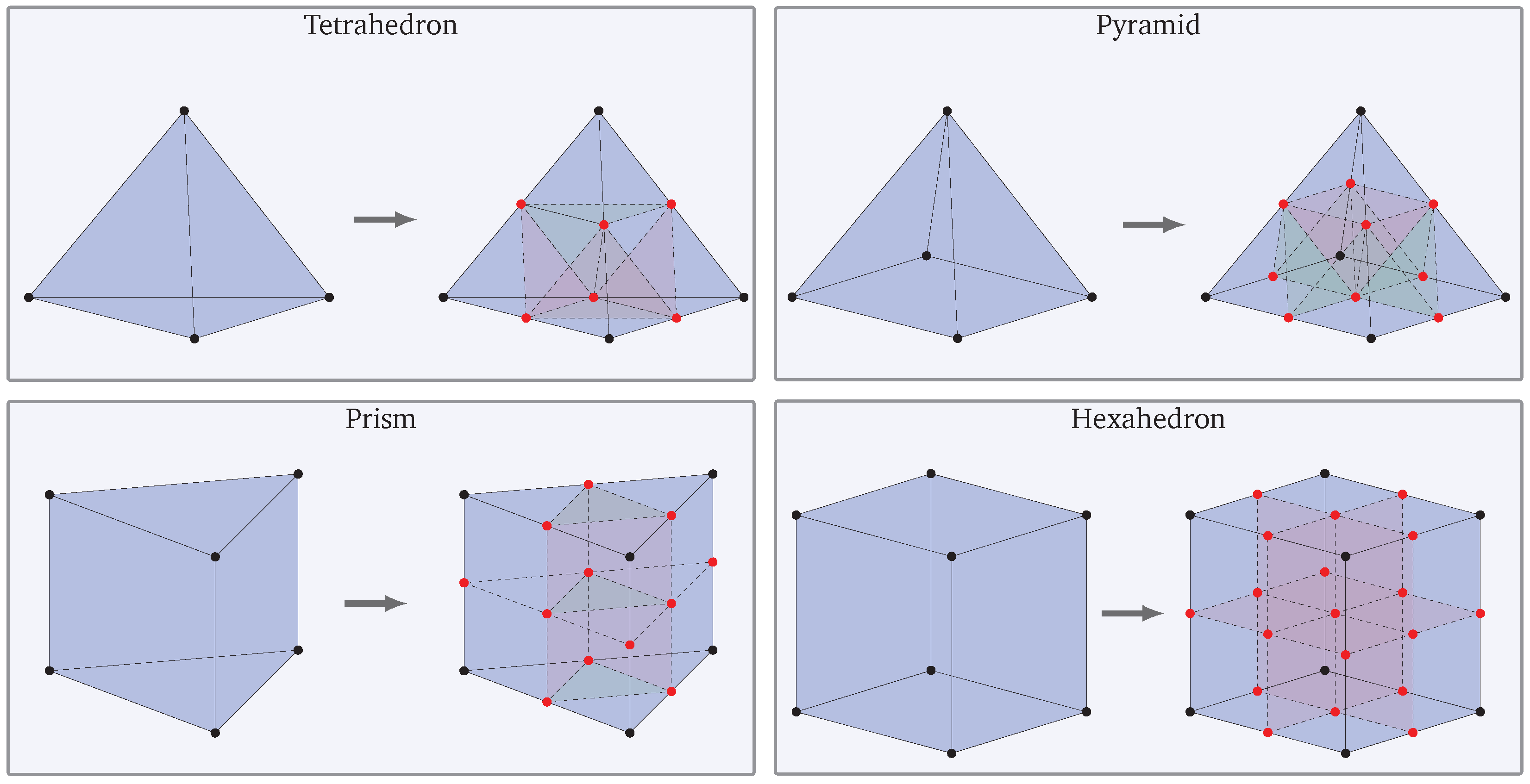
The preprocessor we have developed is capable of refining any kind of element from the background mesh, which makes it more flexible. The preprocessing tool also needs to import the immersed geometry in order to flag the elements that overlap this body for further refinement. This imported geometry is described by STL files. These files contain an unstructured triangulated surface (triangle unit vectors and the coordinates of their corresponding vertices) as generated by the CAD software (we used FreeCAD version 1.1). 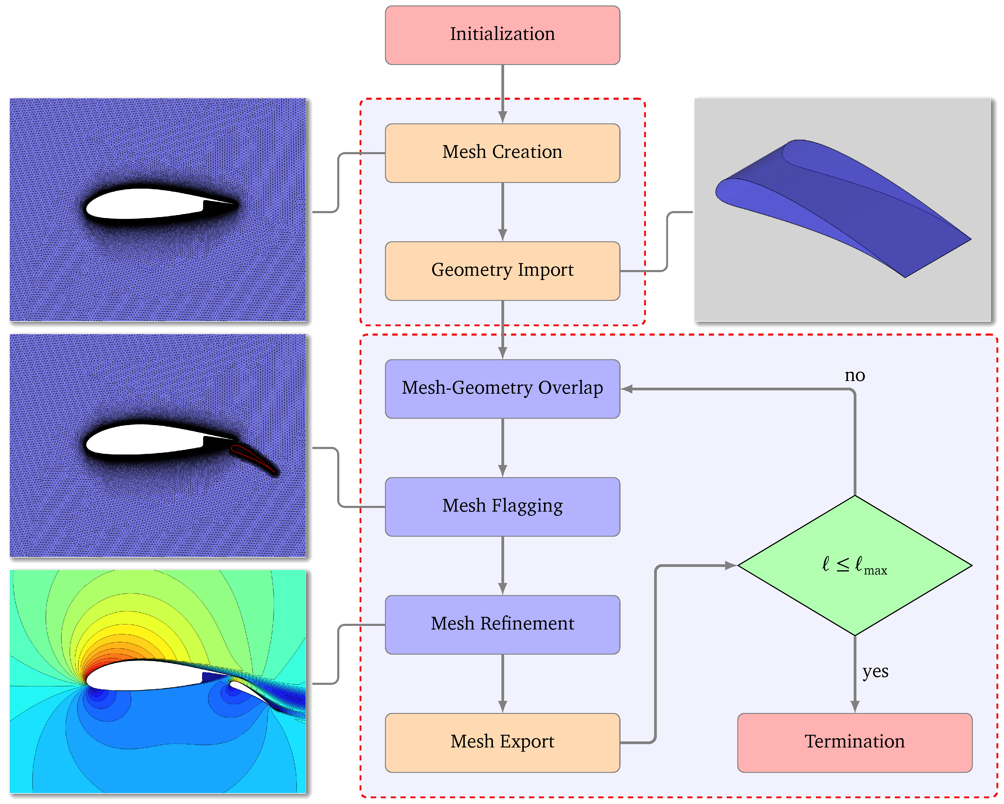In Figure 1 we show the refinement of several types of elements in our preprocessing tool.

The preprocessing tool has the capability of refining the background hexahedral mesh around the triangulated surface of the immersed geometry. The preprocessing tool will follow the next steps for refining the background mesh:

• Marking of the elements that require refinement: For refinement of elements intersecting the triangulated surface of the immersed body, an efficient algorithm for triangle–box overlap has been implemented. Before mesh refinement takes place, this triangle–box overlap is tested for all triangles of the surface triangulation, and if such overlap takes place, the involved elements store the overlapped triangles. During the mesh refinement loop (refinement level $l>0$), this triangle–box overlap is tested only for those elements that store overlapped triangles.
• Marking of the elements for balance: The CODA CFD solver can handle hanging nodes for different types of face elements (triangular and quadrilateral faces). This hanging-node capability is restricted in CODA to elements with a refinement level ratio 2:1. This means that for two neighboring elements with different refinement levels, only a level difference of at most 1 between neighboring cells is allowed. The preprocessing tool is aware of this restriction and therefore an algorithm has been implemented to preserve the balancing of 2:1.
• Refinement of elements: All flagged cells are split into new child cells. Hanging nodes can appear, and the relationship between the face nodes of neighboring elements with different levels of refinement has to be calculated and exported in such a way that CODA can handle them.

In Figure 2 we show the flow diagram of the mesh refinement methodology used in this work. We stress here that the mesh refinement procedure is quite cheap.

3. Results and Discussion

We illustrate the capabilities of our preprocessing tool with an example involving the refinement of the flap region in a multi-element airfoil. The flow around multi-element airfoils is complex, and it is well known to be dominated by different flow mechanisms at different operating conditions, making it rather difficult to accurately predict high-lift flow fields. Regarding flow conditions in this example, the gas has an adiabatic index $\gamma =1.4$ and flows with Reynolds number $\mathrm{Re}=12\times {10}^6$ and freestream Mach number $M=0.2$. Simulations were performed with the airfoil at an angle of attack α = 16°. The non-dimensional density and pressure are set to $\rho =1$ and $p=1$, respectively.

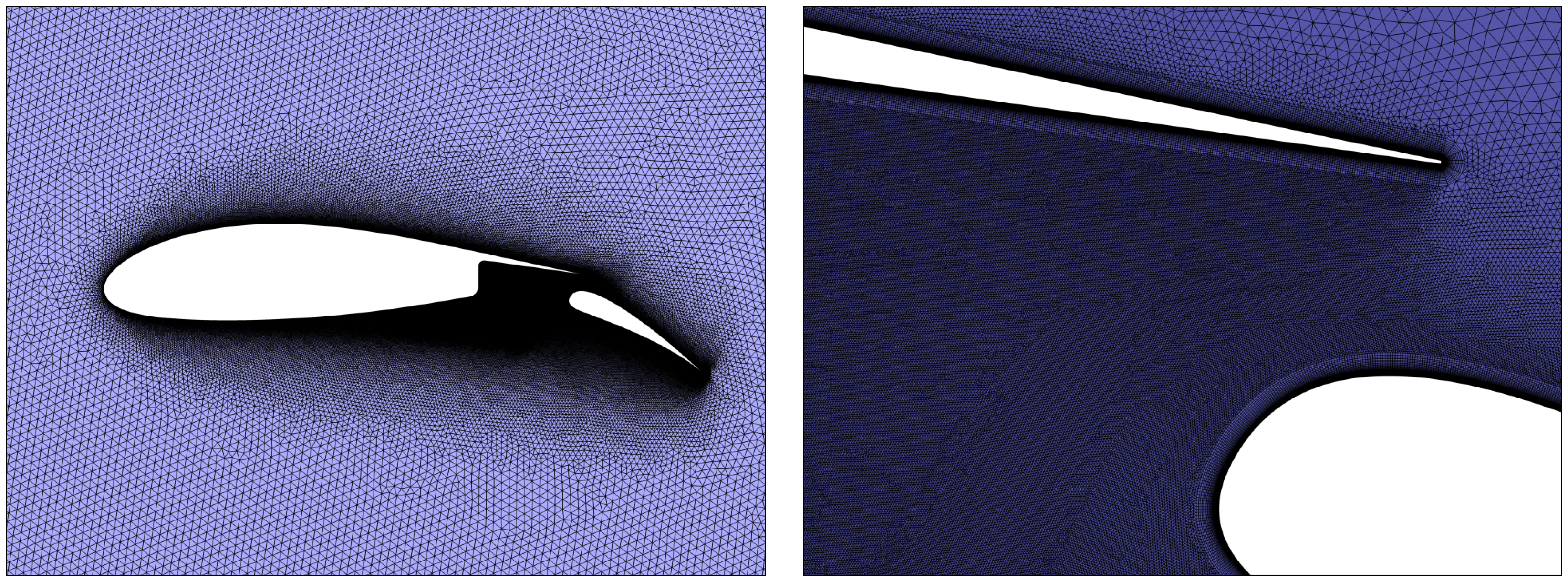
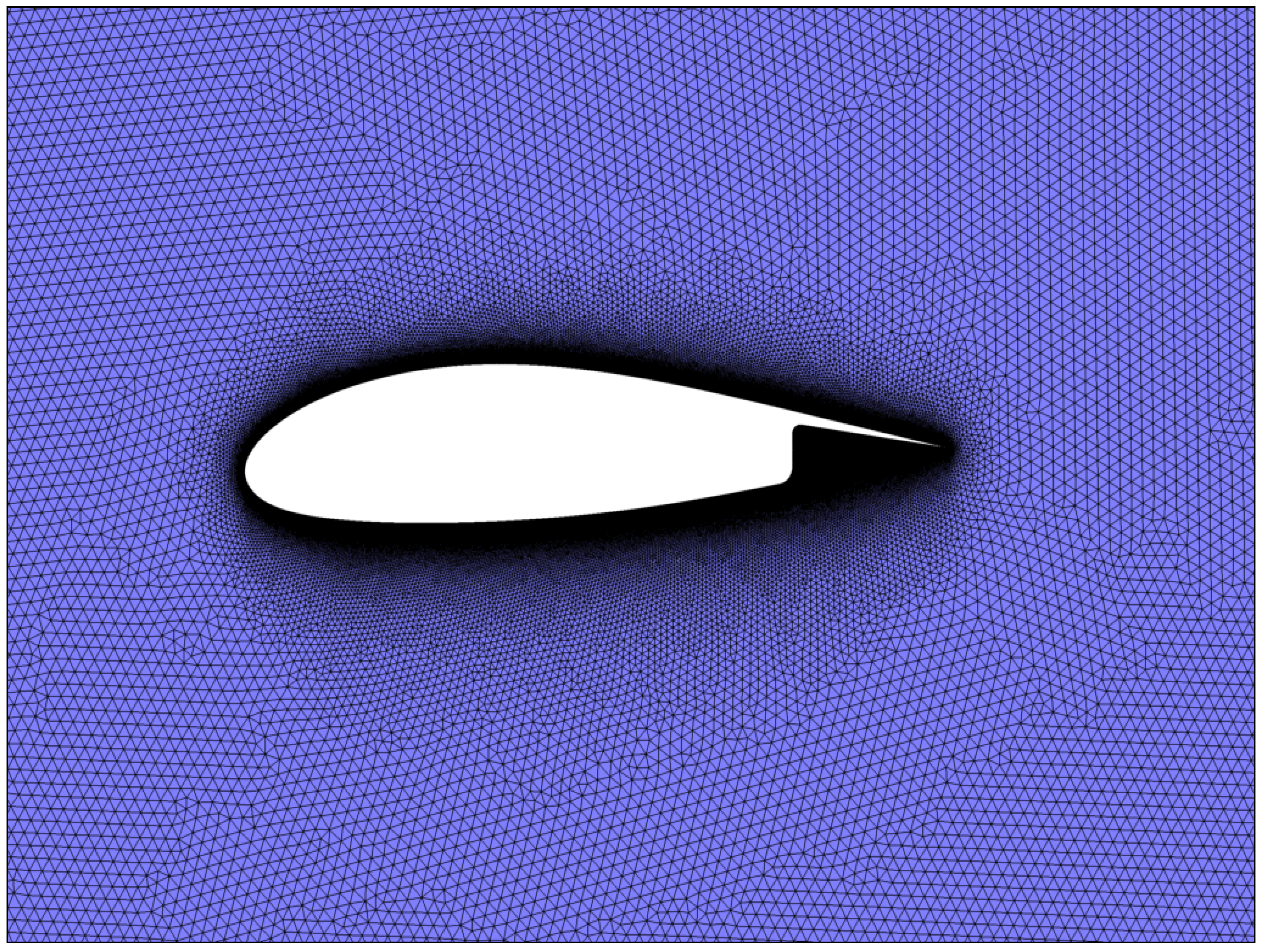
The initial background mesh is a body-fitted mesh for the main part of the airfoil, while the flap is later placed in this background mesh, and the elements that overlap with this immersed geometry are further refined. For comparison purposes, we show the mesh of a full body-fitted airfoil–flap system (see Figure 3) and the initial body-fitted mesh for the main part of the airfoil with an immersed flap (see Figure 4).

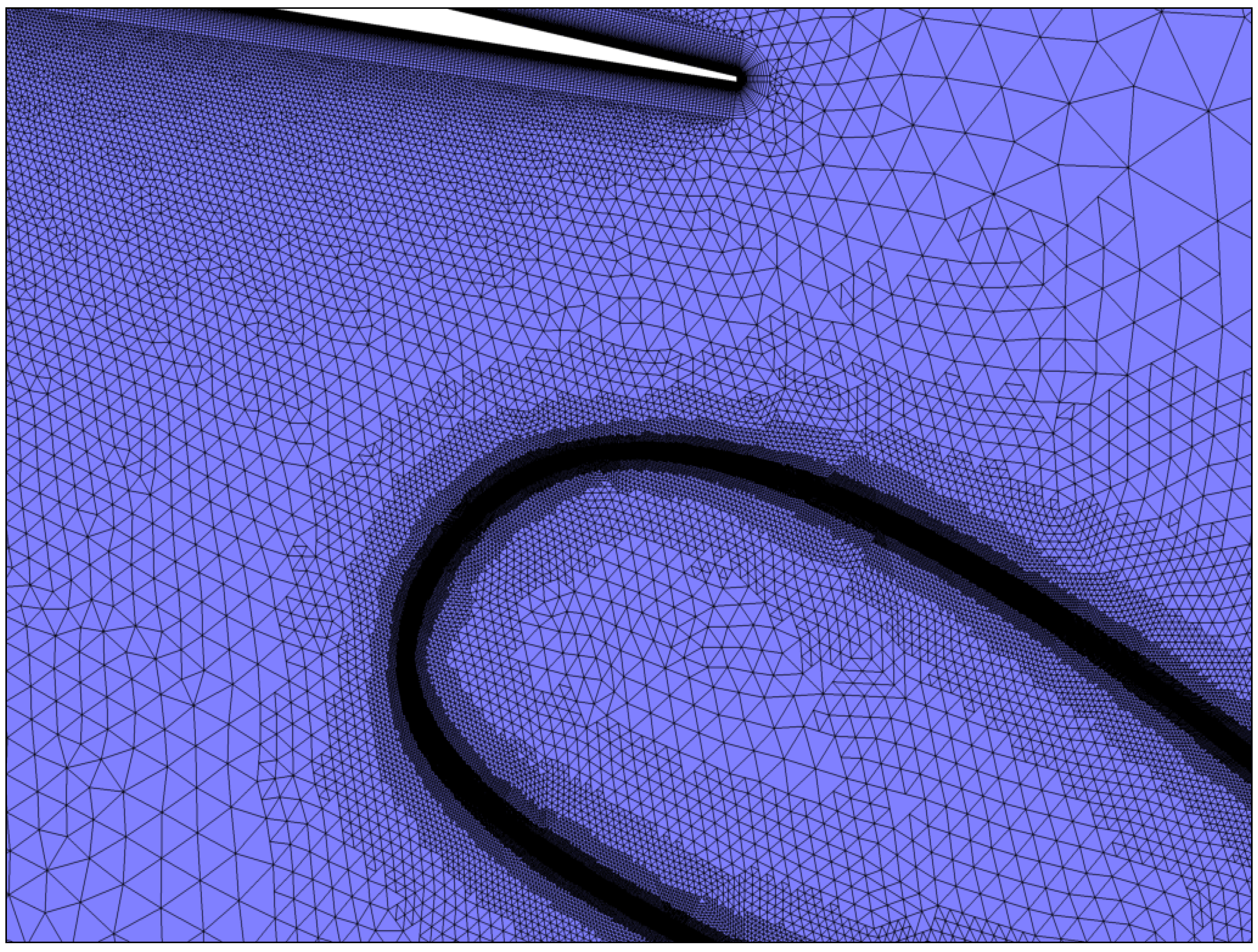
We have performed CFD simulations in both meshes, namely, the mesh of the full body-fitted airfoil–flap system (simulated with pure finite volume schemes) and the initial body-fitted mesh for the main part of the airfoil with an immersed flap (simulated with finite volume schemes along with immersed boundary methods). In Figure 4 we show the body-fitted background mesh of the airfoil, and in Figure 5 a zoomed-in section of the mesh with refinement around the immersed flap. We can observe that the elements in the mesh region where the flap is placed do not conform with the immersed surface. The body-fitted mesh of the airfoil–flap system has around $1.4\times {10}^5$ elements. The numerical simulation of the RANS equations with CODA and using a second-order finite volume spatial discretization operator lasts around 3/4 min on 200 cores. The refined mesh for the initial body-fitted mesh for the main part of the airfoil with an immersed flap has around $1.8\times {10}^5$ elements (coarse mesh) and around $6.3\times {10}^5$ elements (fine mesh), and the numerical simulation with CODA+IBVP lasts around 4/5 min on 200 cores, with similar results with respect to the lift and drag coefficients for the fine mesh (see

Table 1. Lift and drag coefficients for the optimal position of the flap and angle of attack α = 16°. The full body-fitted mesh and the hybrid body-fitted/IBM meshes are considered.

Mesh	CL	CD
Hybrid Body-Fitted/IBM Mesh (Coarse)	1.065849	0.089222
Hybrid Body-Fitted/IBM Mesh (Fine)	1.659730	0.035616
Full Body-Fitted Mesh (Fine)	1.656691	0.033374

).

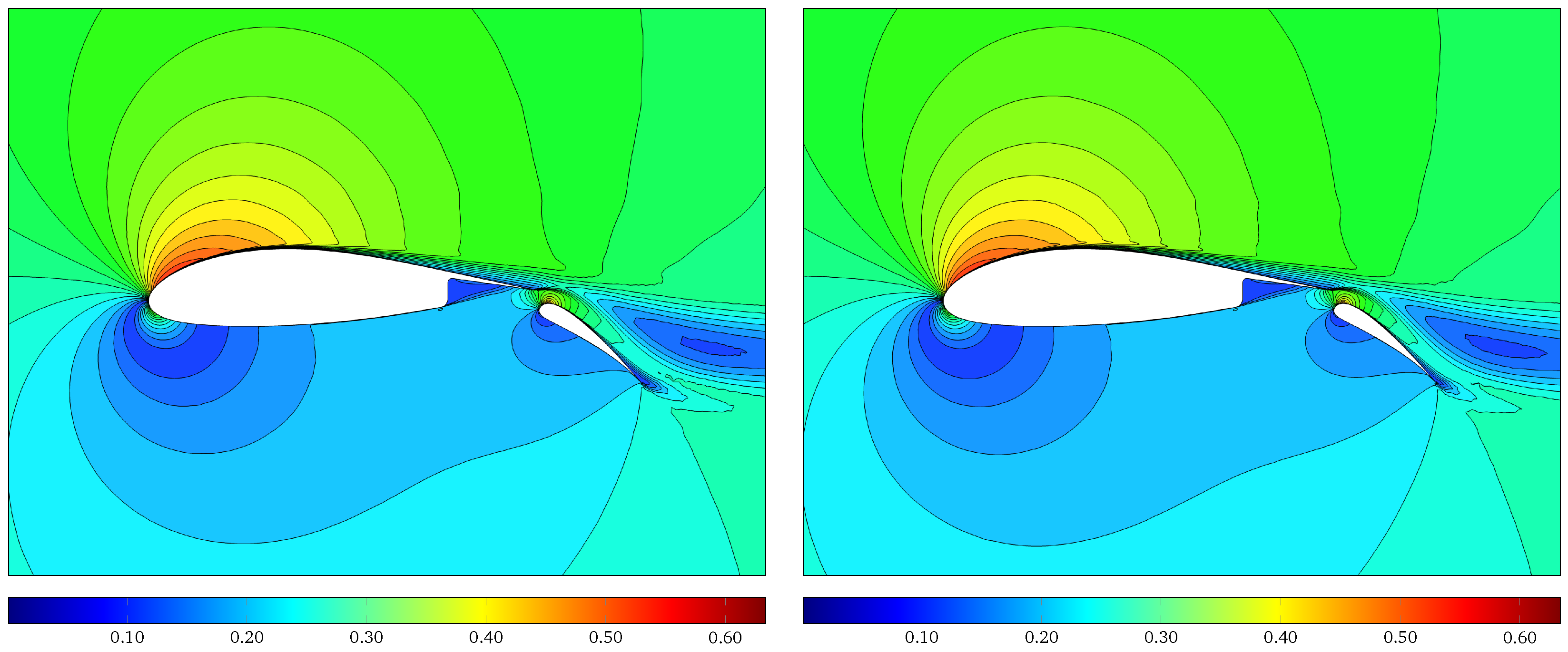
In Figure 6 are shown contour plots of the velocity magnitude for the full body-fitted mesh of the airfoil–flap system (left) and for the body-fitted mesh of the airfoil and IBM mesh for the flap (right). Due to high-lift flow conditions with an angle of attack α = 16°, we can observe the deceleration of the main-element wake behind the flap. A small separation region can be observed near the trailing edge of the flap. We performed simulations for larger angles of attack (α ≈ 18° − 20°), where the flow between the main element wake and flap shear layer becomes increasingly unsteady as stall is approached.

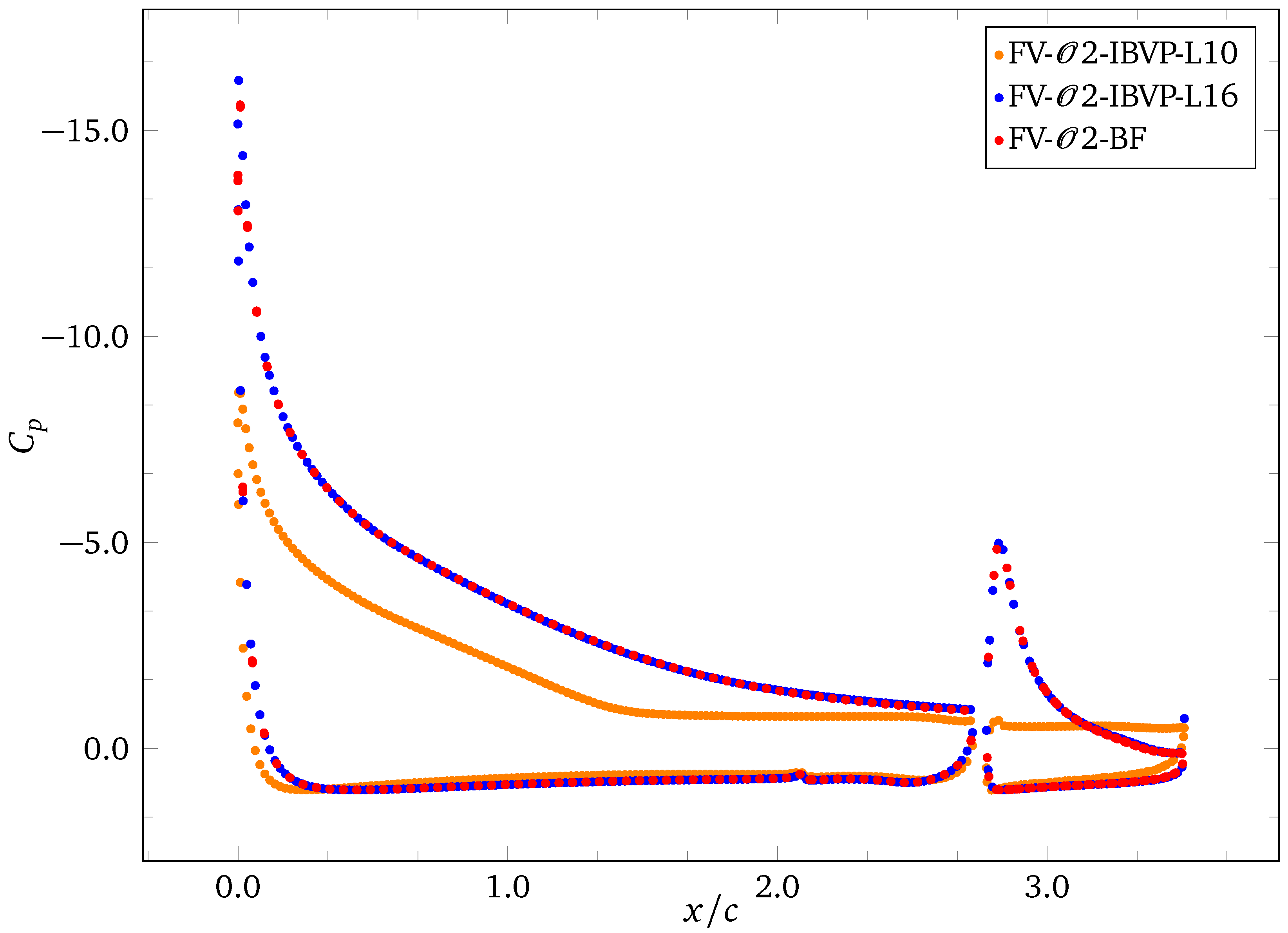
Observe that, if we analyze the pressure coefficient (see Figure 7), for a coarse mesh (low refinement level in the flap region), we get poor results, but for a finer mesh (high refinement level in the flap region) when the hybrid body-fitted/IBM mesh or the full body-fitted mesh for the airfoil–flap system is considered, the results agree well.

In order to accurately simulate the flow past a multi-element airfoil with RANS equations, it is necessary to have a mesh with elements in the boundary layer having a length normal to the surface around ${10}^{-5}$ (or even smaller). An IBM mesh with elements in the boundary layer for the wing and the flap having a similar size requires around $2.5\times {10}^6$ elements. Therefore, in a coarse IBM mesh, we expect a large discrepancy in the flow field properties compared to very fine meshes (body-fitted meshes or IBM meshes). We have observed in several numerical experiments that even if the mesh in the boundary layer of the wing is very fine but coarse in the boundary layer of the flap, the simulations predict unreliable values of the physical quantities, as can be seen in Figure 7 for the case of the pressure coefficient. The mesh resolution and also the geometry tessellation resolution play an important role when we simulate the flow around a multi-element airfoil with RANS equations. More details on the effect of the mesh resolution of IBM meshes on aerodynamic simulations can be found in references [1,7].

Regarding the mesh characteristics, some elements in the refined region are tetrahedra and some are pyramids/hexahedra, so the hybrid mesh adaptation tool works pretty well on all these types of element. These results show the effectiveness of our mesh refinement approach for complex unstructured background meshes. It is no longer necessary to use only Cartesian background meshes with immersed boundary methods.

The preprocessing tool presented in this article works for 2D and 3D meshes. The example discussed in this section is a 2D case but using 3D meshes with only one element in the extrusion direction. It is important to mention that for complex 3D configurations, the preprocessing tool can refine unstructured hybrid meshes up to 300 million elements. The main drawback when applying the IBVP method to this kind of complex geometries is the huge amount of elements required to simulate flow problems. For example, a RANS simulation of the CRM aircraft with a body-fitted mesh requires around 200 million elements while one with IBVP requires around 2500 million elements [7].

4. Conclusions

In this work, we have presented the development and application of a mesh adaptation tool on hybrid unstructured meshes for immersed boundary volume penalization methods in the CODA computational fluid dynamics solver. Our preprocessing tool can refine any kind of element from an imported mesh generated by an external mesh generator, like GMSH. This allows us to simulate fluid flow problems with the immersed boundary method not only on Cartesian meshes, but on general hybrid unstructured meshes. As an example of application, we perform the simulation of the subsonic flow past a multi-element airfoil by solving the Reynolds-averaged Navier–Stokes equations on unstructured body-fitted meshes along with immersed geometries. The numerical simulations reported are in good agreement with their corresponding full body-fitted meshes.