A Machine Learning Approach to Predicting the Climate Impact of North Atlantic Flights ^†

Abstract

Aviation emissions significantly contribute to climate change, with both CO₂ and non-CO₂ effects, such as contrails and nitrogen oxides. The aim of this paper was to develop a machine learning-based model to predict the climate impact of flights using atmospheric and emissions data. The proposed model, an LGMB Regressor algorithm, was trained on a dataset of atmospheric variables and algorithmic Climate Change Functions to forecast the cumulative impact of these emissions measured via the total average temperature response at 20 years (ATR20). In a test on five months of data pertaining to the North Atlantic Corridor, the LGBM Regressor model exhibited strong predictive performance, with an $R^2$ score between 0.41 and 0.55 and a Mean Absolute Percentage Error between 2.68% and 5.11% depending on the month. This study shows the potential of machine learning to provide efficient, accurate climate impact assessments for aviation.

1. Introduction

Aviation emissions are a significant contributor to climate change, with non-CO₂ effects—such as nitrogen oxides (NO_X) and contrails—having been estimated to account for two-thirds of the sector’s climate impact in 2018 from emissions since 1940 [1]. Quantifying this impact is complex because, unlike long-lived CO₂ effects, non-CO₂ effects operate on short timescales and are highly dependent on local atmospheric conditions [1,2,3].

The climate impact of a flight is often quantified in terms of CO2-equivalent emissions calculated from climate metrics. While metrics such as Radiative Forcing (RF) and Global Warming Potential (GWP) are widely used, the Average Temperature Response (ATR) provides a valuable link between emissions and subsequent warming by measuring cumulative temperature change over a specific period (e.g., 20 years) [4,5]. Calculating these metrics traditionally requires computationally expensive physical models. Algorithmic Climate Change Functions (aCCFs) and the Contrail Cirrus Prediction Tool (COCIP) are simplified models that accelerate computation through interpolation while accounting for the main physical processes [6,7,8].

This article presents a condensed version of the report we prepared within the SJU-funded AEROPLANE project on a machine learning (ML) approach to efficiently predicting the climate impact of individual flights, bypassing the high computational costs of physical models [9]. We trained ML algorithms on a comprehensive dataset, which incorporates detailed metrics for both CO₂ and non-CO₂ impacts under various weather conditions.

2. Data

The dataset of atmospheric data used in this study covers the North Atlantic airspace corridor, spanning latitudes ${20}^{\circ }$ to ${80}^{\circ }$ and longitudes −${80}^{\circ }$ to $0^{\circ }$, with a $0.5^{\circ }$ grid size for both latitude and longitude, and three pressure levels—200, 225, and 250 millibars—corresponding approximately to altitudes of 10, 11, and 12 kilometers. The time span of the collected data covers every day in January 2019, with 6-hour intervals. The source of the data is the ERA5 hourly data on pressure levels available from the Copernicus Data Store [10,11].

The final dataset includes 11 variables, which are described below. The first nine in the list are atmospheric variables available from the Copernicus Data Store and used as input tfor the algorithmic Climate Change Functions (aCCFs). The others were computed as part of the activities of the AEROPLANE project (cf. [12,13] for details about the approach adopted and the model used).

1.

Surface Short-Wave (Solar) Radiation Downwards (ssrd)—Incoming solar radiation per unit surface over an hourly timestep (unit: $\mathrm{J} {\mathrm{m}}^{-2}$).

2.

Top Net Long-Wave (Thermal) Radiation (ttr)—Net thermal radiation at the top of the atmosphere (unit: $\mathrm{J} {\mathrm{m}}^{-2}$).

3.

Potential Vorticity (pv)—A dynamic quantity conserved for an air parcel moving adiabatically and used by the aCCFs to identify the tropopause level (units: $\mathrm{K} {\mathrm{m}}^2 {\mathrm{kg}}^{-1} {\mathrm{s}}^{-1}$).

4.

Geopotential (z)—Gravitational potential per unit mass, which is used by the aCCFs to identify the tropopause level (unit: $\mathrm{kg} {\mathrm{kg}}^{-1}$).

5.

Air Temperature (t)—Recorded in Kelvin (unit: K).

6.

Specific Humidity (q)—Mass of water vapor per unit mass of air (units: $\mathrm{kg} {\mathrm{kg}}^{-1}$).

7.

Relative Humidity (r)—The amount of moisture in the air compared to what the air can hold at that temperature (unit: %).

8.

Eastward Wind (u)—Wind component from west to east (unit: $\mathrm{m} {\mathrm{s}}^{-1}$).

9.

Northward Wind (v)—Wind component from south to north (unit: $\mathrm{m} {\mathrm{s}}^{-1}$).

10.

Persistent Contrail Formation Areas (pcfa)—Regions that, according to aCCF predictions, will form persistent contrails, derived from meteorogical data (boolean).

11.

Average Temperature Response with a 20-year Time Horizon (ATR20, target variable)—The total ATR with a 20-year time horizon per unit fuel consumption, combining the effects of all individual emissions, measuring the impact that an A320 aircraft would have by traveling through a region at a specific latitude, longitude, altitude, and time (unit: K kg [fuel]⁻¹).

The entire dataset contains hundreds of millions of rows when flattened from its multi-indexed format, highlighting the vast scale of information being handled. A scalable solution is therefore necessary to efficiently analyze, pre-process, and transform the data and train our model on it.

3. Experimental Setup

The variables in Section 2 represent the final set of features used for model training after feature selection, addressing multicollinearity and the application of dimensionality reduction techniques. All necessary data pre-processing steps performed are detailed in the full report [9], which also includes a discussion on the necessity of feature scaling and various feature-scaling techniques. In this section, we focus on model selection and training and improving the model-training results.

3.1. Model Selection and Training

Our approach consisted of the following process: finding the best baseline model, improving the model’s performance by identifying and removing outliers, and finding models that could be used for outlier values. Due to the size of the dataset, we chose to use separate monthly models.

We tested a total of 16 different algorithms, namely, LGBM Regressor, Linear Regression, Ridge, Lasso, Decision Tree, Random Forest, Gradient Boosting, AdaBoost, BayesianRidge, CatBoost, ElasticNet, ExtraTrees, Huber, KNN, RANSAC, and XGBoost.

The LGBM Regressor consistently outperformed the other algorithms, demonstrating better predictive capability for the aggregated ATR20 variable. Hence, the LGBM Regressor was chosen as the baseline model. LGBM Regressor is a high-performance gradient-boosting framework developed by Microsoft, specifically designed for efficiency and scalability [14]. It is based on decision tree algorithms, efficiently handles missing values, uses histogram-based learning and a leaf-wise growth strategy, and is optimized for large datasets with high-dimensional features.

3.1.1. Baseline-Model Results

Table 1. Performance of monthly LGBM Regressor model as measured by MSE, $R^2$, MAE, and MAPE.

Model	Scaler	Month	MSE, (K/kg)2	${\mathit{R}}^2$	MAE, K/kg	MAPE,%
LGBM	No Scaler	January	$1.29\times {10}^{-26}$	0.37	$2.96\times {10}^{-14}$	10.44
LGBM	No Scaler	June	$5.04\times {10}^{-27}$	0.40	$1.77\times {10}^{-14}$	9.91
LGBM	No Scaler	July	$4.90\times {10}^{-27}$	0.39	$1.89\times {10}^{-14}$	17.6
LGBM	No Scaler	September	$7.77\times {10}^{-27}$	0.37	$2.18\times {10}^{-14}$	8.65
LGBM	No Scaler	December	$1.39\times {10}^{-26}$	0.32	$3.09\times {10}^{-14}$	9.42

shows the monthly performance (for January, June, July, September, and December) of the LGBM Regressor, which was selected as the baseline model (hereinafter referred to as ‘model B’) because it always outperformed the other algorithms (for details on the other algorithms, please refer to our full report [9]). We used the following metrics: MSE (Mean Squared Error), $R^2$ (Coefficient of Determination), MAE (Mean Absolute Error), and MAPE (Mean Absolute Percentage Error).

The discussion below focuses on the steps taken to improve model performance. These steps include outlier detection and model adjustment.

3.1.2. Outlier Detection

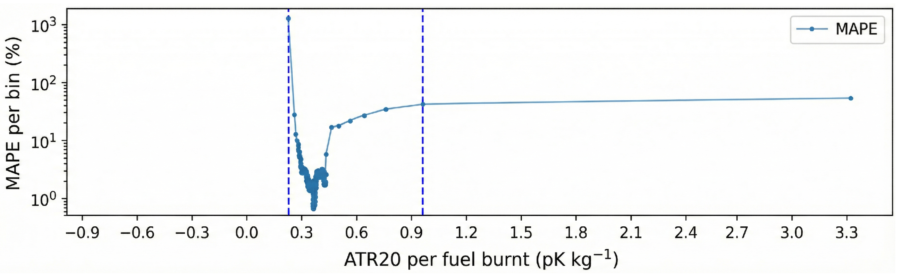
Outlier detection aims at identifying data points that significantly deviate from the overall distribution and impact model performance. Outliers can arise due to measurement errors, rare events, or natural variability in data. Analysis of input features did not result in identification of specific outlier values or patterns. At the same time, we noticed that low-frequency values in the tails of the distribution of ATR20 in the target set significantly contributed to the model error rate. The bulk of the ATR20 distribution for the entirety of 2019 is approximately in the range between 0.2 and 1.0 pK, while only about 1% of the values fall outside this range [9]. Our hypothesis is that these outliers are rare enough that the model fails to reproduce them, leading to large prediction errors, as further observed during model evaluation. Figure 1 shows the analysis of the June 2019 data as an example. The distributions of the other months are very similar for the data for the other months in 2019. The figure displays the average MAPE in 100 bins of the target variable, ATR20. This indicates that the model fails to accurately predict the very low and very high ATR20 values, with percentage errors higher than 50%. The largest errors occurred on the data points where the value of pcfa feature is 1. In total, approximately 1% of the points in the dataset were identified as outliers with this approach.

3.1.3. Results After Outlier Removal

Removing the outlier values and re-training the algorithm on the remaining 99% of the dataset significantly improved LGBM Regressor performance. Depending on the month, the MAPE decreased by a factor between 1.8 and 6.0, while $R^2$ increased by a factor of 1.3–1.4. The results for all metrics and months for the model trained after the outliers were removed are summarized in

Table 2. Change in LGBM Regressor performance after the outliers were removed (model M) compared to the baseline model (model B).

Model	Month	Metric	Baseline Model	Model After Removing Outliers
LGBM	June	R2	0.40	0.55
		MAE	$1.77\times {10}^{-14}$	$1.14\times {10}^{-14}$
		MAPE (%)	9.91	2.68
LGBM	July	R2	0.39	0.52
		MAE	$1.89\times {10}^{-14}$	$1.30\times {10}^{-14}$
		MAPE (%)	17.60	3.15
LGBM	September	R2	0.37	0.50
		MAE	$2.18\times {10}^{-14}$	$1.53\times {10}^{-14}$
		MAPE (%)	8.65	3.36
LGBM	December	R2	0.32	0.41
		MAE	$3.09\times {10}^{-14}$	$2.35\times {10}^{-14}$
		MAPE (%)	9.42	5.12

. This model will be referred to as “model M” hereinafter.

Additionally, after the removal of the outliers, we observed an improvement in the performance of the models trained using other algorithms that were tested while selecting the baseline model, but LGBM remained the best-performing algorithm.

The above results indicate that the LGBM Regressor captures between 41% and 55% of the variance in the target variable (with model B and model M, respectively), which is a moderately good score. This result was obtained with the entire dataset regardless of the ‘pcfa’ value. If we restrict the scope to the set of data with pcfa = 0, the $R^2$ increases to 97%, indicating that most of the discrepancies are in regions of persistent contrail formation, in which the cumulated climate impact of a flight is very sensitive to the local conditions. However, the value of $R^2$ alone does not tell us how well the model performs for each prediction. In particular, $R^2$ scores of around 0.5 (cf. Table 2), combined with MAE values of only a few hundredths of the typical signal ($\approx {10}^{-14}$ compared to $\approx {10}^{-12}$, respectively) and MAPE values of 3–5%, indicate a low average deviation and high prediction accuracy. Model M generally performs well. For instance, for the June model, 94.22% of the data points have an MAPE of up to 10%, whereas 2.25%, 2.95%, and 0.59% of the data points have MAPE values between 10% and 20%, between 20% and 50%, and above 50%, respectively. The other monthly models have a similar error distribution.

To determine whether the higher-error cases (MAPE above 50%) are associated with a specific geographical location, we compared the actual and predicted values in the North Atlantic across different dates and pressure levels.

The smallest number of such errors was found at 200 hPa, and they are concentrated at latitudes lower than 70° N (June). The largest frequency of errors greater than 50% was found at 250 hPa, with these data points concentrated at higher latitudes, between 50° N and 80° N (for visualizations and details, please refer to our full report [9]). The presence of discrepancies suggests room for further refinement in local predictions, especially in handling outlier cases.

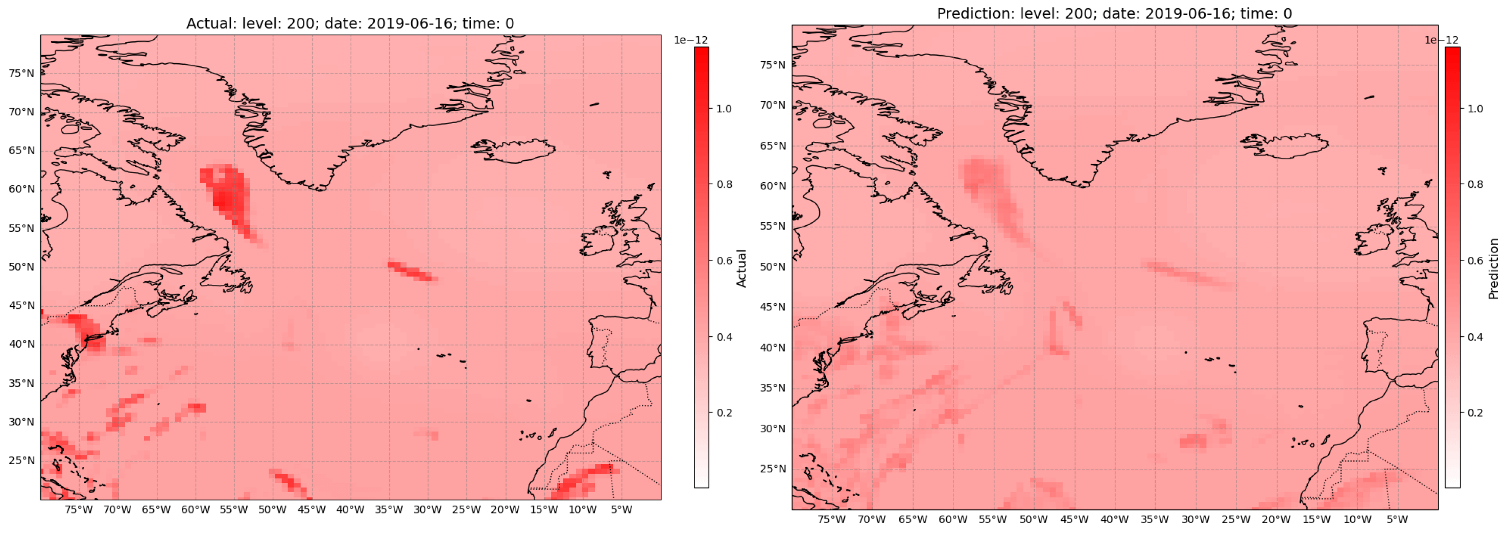
Figure 2 shows a sample comparison of ‘actual’ ATR20 values with the ‘predicted’ ATR20 values computed with our ML model for a particulate date, hour, and pressure level. As can be seen from the plots, the model accurately captures the overall spatial pattern of aggregated ATR20 values across the North Atlantic region and, thus, generalizes well across different spatial locations, time periods, and pressure levels. Some discrepancies between predicted and actual values exist, suggesting that there may be some complex local factors or rare atmospheric conditions that the model struggles to reproduce. However, the model’s ability to adapt to varying atmospheric conditions and accurately predict ATR20 values suggests its potential for reliable climate impact assessments in aviation route planning.

3.1.4. Handling Outliers

As described in Section 3.1.2, we identified the subset of target data in the bottom 0.5% and in the top 99.5% of the ATR20 distribution as outlier values significantly impacting the model’s performance. As these data points all occur for pcfa = 1, they correspond to regions where the atmospheric conditions are apt for persistent contrail formation according to the physical model. The climate impact of such contrails (combined with that of CO₂ and other non-CO₂ effects) is close to 0 or negative (i.e., cooling contrails) for the bottom 0.5 percentile of the distribution, whereas it is high (i.e., strongly warming contrails, potentially “big hits” [15]) for the top 99.5 percentile. In the following, we characterize the data points contributing to these extreme values of the target variable through the input features based on June 2019 data. For this purpose, we compared feature distributions and other statistical parameters for the following three data classes: (1) upper outliers—ATR20 values greater than or equal to the 99.5th percentile and for which pcfa = 1 (the share of values is approx. 0.499%); (2) lower outliers—ATR20 values less than or equal to the 0.5th percentile and for which pcfa = 1 (the share of values is approx. 0.499%); and (3) non-outliers—the remaining values (the share of values is approx. 99.002%).

We performed distribution analysis of the input features of the three data classes to determine whether the three classes of ATR20 have the characteristics that can be identified through the input features, i.e., without knowledge of the corresponding ATR20. Our analysis showed that there is no single variable, among the input features of the ML algorithm, that enables us to separate the three data classes. However, there are certain data patterns that, if combined, might make this task feasible. Thus, it is possible to apply classification algorithms to identify the outlier class to which a particular data point belongs and, subsequently, apply alternative models to predict ATR20 for points in each specific class.

• Classification Model Training and Results

We chose RandomForestClassifier to predict whether a given data point is an outlier. RandomForestClassifier is an ensemble-learning method from the scikit-learn library that belongs to the family of bagging algorithms [16]. It is based on Decision Trees and operates by constructing multiple decision trees during training and aggregating their predictions to improve accuracy and reduce overfitting. The training process consisted of the following steps (for details, please refer to our full report [9]). (1) Data labeling: Observations derived from the dataset were labeled and assigned to the following classes—0, non-outlier; 1, upper outlier; and 2, lower outlier. (2) Feature scaling: Because of the different value scales of the input features, we standardized the data using scikit-learn StandardScaler. (3) Resampling: As the outlier values represent minority classes, we used resampling to rebalance the dataset with SMOTE (Synthetic Minority Over-Sampling Technique) [17]. (4) Model training: We trained the RandomForestClassifier model on monthly datasets.

The RandomForestClassifier results showed high overall accuracy with an f1-score that, depending on the month, ranged from 0.97 to 0.98. In particular, it demonstrated high accuracy in predicting non-outlier values (with an f1-score of 0.99) and a particularly high accuracy in predicting upper (with an f1-score between 0.81 and 0.83) and lower (with an f1-score between 0.82 and 0.85) outlier values.

We subsequently determined the best models with which to predict ATR20 values for the upper-outlier class and lower-outlier class. Unlike with models B and M, the dataset’s size allowed us to train the models based on all values falling into the outlier categories for the whole year. For upper outliers, LGBM Regressor was selected as the best model (Model U). For Lower outliers, BayesianRidge with RobustScaler was selected as the best model (Model L). The combination of models L, M, and U was used to predict ATR20, as described in Section 4.

4. Final Results

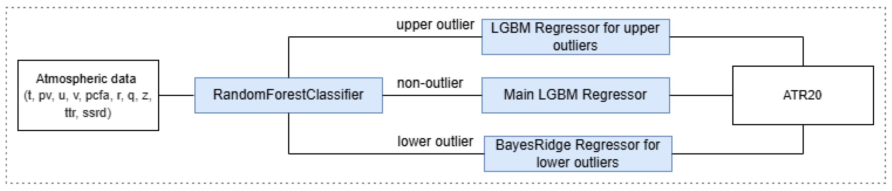
Figure 3 represents the proposed combined pipeline for predicting ATR20 values. The result of this approach is model C, which combines a Random Forest Classifier that uses the set of input features to split the dataset into three classes of data points: non outliers, lower outliers, and upper outliers. For each of these classes, different models are used to predict ATR20: model M, model L, and model U, respectively.

We tested the suggested combined approach on the data for June 2019 that was not included in training for models M, U, and L: first, the data was classified to define the group it belongs to (upper outlier, non-outlier, or lower outlier); then, the appropriate model was applied for predicting ATR20 values. The MAPE and $R^2$ of model C based on the tested data are 4.24% and 0.54, respectively. This is an improvement compared to both our baseline model (model B) and the model trained only on the non-outlier dataset (model M).

Table 3. Comparison of performance of the combined model (C) with the baseline model (B) and main model (M).

Model	Month	MSE, K/kg2	${\mathit{R}}^2$	MAE, K/kg	MAPE,%
model C	June	$2.27\times {10}^{-27}$	0.54	$1.25\times {10}^{-14}$	4.24
model B	June	$4.63\times {10}^{-27}$	0.41	$1.68\times {10}^{-14}$	10.43
model M	June	$4.81\times {10}^{-27}$	0.37	$1.56\times {10}^{-14}$	10.16

shows a summary of the results.

The LGBM Regressor’s success in this context can be attributed to several factors. Firstly, LGBM does not make assumptions about the underlying data distribution, making it well suited for the complex, non-linear relationships often present in meteorological data. Secondly, LGBM makes predictions using gradient-boosted decision trees, which split the data based on feature values rather than distances in feature space. This approach allows the model to capture complex, nonlinear relationships between atmospheric and impact variables while efficiently handling large datasets.

ATR20 Predictions for Transatlantic Flights

We tested the model’s potential to assess climate impact along the trajectories of 37 flights between JFK New York and London Heathrow airports based on forecast weather data obtained from the ECMWF’s Meteorological Archival and Retrieval System (MARS) for June and September 2019. We applied the model to the respective forecast weather data at the geographical points (latitude, longitude, and pressure level) along the following flights’ trajectories and at the specific moment in time: Filed Flight Points, Actual Flight Points and Great Circular Distance. The mean percentage prediction error for these flights along these trajectory types ranged between −5.34% and 5.65%, i.e., within the range of uncertainty of the physical model (cf. [13] for details).

5. Limitations and Future Work

This study’s limitations highlight key directions for future work, primarily the need to validate the model using real-world aircraft trajectories instead of just gridded data. Recommendations include expanding the dataset to cover multiple years and diverse geographical regions, potentially training models on seasonal or geographic clusters rather than individual months. Future research should also explore predicting the individual components of the ATR20 rather than only the aggregate value, which would enhance model flexibility and characterization. Further refinements are needed in validating the model against more complex physical models (like CCFs), improving the handling of data outliers, and increasing model interpretability using methods like SHAP, with the ultimate goal of integrating the model into operational tools.

6. Conclusions

This study successfully developed a machine learning model, primarily using the LGBM Regressor, to predict aviation’s climate impact (ATR20), achieving R² scores of between 0.41 and 0.55 and MAPE errors between 2.68% and 5.11% on the main dataset. The research also demonstrated a hybrid approach using a RandomForestClassifier to effectively identify and handle outliers with separate models, enhancing accuracy. A key achievement is the model’s significant computational speed, with monthly main model training and an inference of under one hour on a typical laptop, making it feasible to integrate climate impact predictions into routine flight planning and air traffic management. Although further research is needed to broaden its applicability, this work confirms the potential of ML to accurately and efficiently assess the climate impact of individual flights without relying on computationally demanding physical models.

References

1. Lee, D.; Fahey, D.; Skowron, A.; Allen, M.; Burkhardt, U.; Chen, Q.; Doherty, S.; Freeman, S.; Forster, P.; Fuglestvedt, J.; et al. The contribution of global aviation to anthropogenic climate forcing for 2000 to 2018. Atmos. Environ. 2021, 244, 117834. [Google Scholar] [CrossRef] [PubMed]
2. Kahn Ribeiro, S.; Newman, P.; Dhar, S.; Diemuodeke, O.E.; Kajino, T.; Lee, D.S.; Nugroho, S.B.; Ou, X.; Hammer Strømman, A.; Whitehead, J. Chapter 10: Transport; Cambridge University Press: Cambridge, UK; New York, NY, USA, 2022; pp. 2273–2318. [Google Scholar]
3. Rao, P.; Yin, F.; Grewe, V.; Yamashita, H.; Jöckel, P.; Matthes, S.; Mertens, M.; Frömming, C. Case Study for Testing the Validity of NOx-Ozone Algorithmic Climate Change Functions for Optimising Flight Trajectories. Aerospace 2022, 9, 231. [Google Scholar] [CrossRef]
4. Borella, A.; Boucher, O.; Shine, K.P.; Stettler, M.; Tanaka, K.; Teoh, R.; Bellouin, N. The importance of an informed choice of CO2-equivalence metrics for contrail avoidance. EGUsphere 2024, 2024, 1–24. [Google Scholar] [CrossRef]
5. Grewe, V.; Dahlmann, K.; Flink, J.; Frömming, C.; Ghosh, R.; Gierens, K.; Heller, R.; Hendricks, J.; Jöckel, P.; Kaufmann, S.; et al. Mitigating the Climate Impact from Aviation: Achievements and Results of the DLR WeCare Project. Aerospace 2017, 4, 34. [Google Scholar] [CrossRef]
6. van Manen, J.; Grewe, V. Algorithmic climate change functions for the use in eco-efficient flight planning. Transp. Res. Part Transp. Environ. 2019, 67, 388–405. [Google Scholar] [CrossRef]
7. Schumann, U. A contrail cirrus prediction model. Geosci. Model Dev. 2012, 5, 543–580. [Google Scholar] [CrossRef]
8. Teoh, R.; Schumann, U.; Gryspeerdt, E.; Shapiro, M.; Molloy, J.; Koudis, G.; Voigt, C.; Stettler, M.E.J. Aviation contrail climate effects in the North Atlantic from 2016 to 2021. Atmos. Chem. Phys. 2022, 22, 10919–10935. [Google Scholar] [CrossRef]
9. D1.3-Machine-Learning Prediction Report. Technical Report, AEROPLANE Consortium, 2025. Available online: https://drive.google.com/file/d/1-v0C1-Y75Q82oLvla-vhxc2N5Q7fvlNk/view?usp=sharing (accessed on 12 April 2026).
10. Hersbach, H.; Bell, B.; Berrisford, P.; Biavati, G.; Horányi, A.; Muñoz Sabater, J.; Nicolas, J.; Peubey, C.; Radu, R.; Rozum, I.; et al. ERA5 hourly data on pressure levels from 1940 to present. Copernic. Clim. Change Serv. (C3s) Clim. Data Store (Cds) 2023, 10, 24381. [Google Scholar] [CrossRef]
11. Hersbach, H.; Bell, B.; Berrisford, P.; Biavati, G.; Horányi, A.; Muñoz Sabater, J.; Nicolas, J.; Peubey, C.; Radu, R.; Rozum, I.; et al. ERA5 hourly data on single levels from 1940 to present. Copernic. Clim. Change Serv. (C3s) Clim. Data Store (Cds) 2023. [Google Scholar] [CrossRef]
12. D1.2-Climate Metrics Report. Technical Report, AEROPLANE Consortium, 2024. Available online: https://ec.europa.eu/research/participants/documents/downloadPublic?documentIds=080166e5146e7046&appId=PPGMS (accessed on 12 April 2026).
13. D1.4-Climate Metrics Post-Operation Analysis. Technical Report, AEROPLANE Consortium, 2025. Available online: https://drive.google.com/file/d/1oEB0V_Mx7h5wQSn5-RO1QJc7vW4VxScB/view?usp=sharing (accessed on 12 April 2026).
14. Ke, G.; Meng, Q.; Finley, T.; Wang, T.; Chen, W.; Ma, W.; Ye, Q.; Liu, T. LightGBM: A Highly Efficient Gradient Boosting Decision Tree. Neural Inf. Process. Syst. 2017, 30, 3146–3154. [Google Scholar]
15. Wilhelm, L.; Gierens, K.; Rohs, S. Meteorological Conditions That Promote Persistent Contrails. Appl. Sci. 2022, 12, 4450. [Google Scholar] [CrossRef]
16. Pedregosa, F.; Varoquaux, G.; Gramfort, A.; Michel, V.; Thirion, B.; Grisel, O.; Blondel, M.; Prettenhofer, P.; Weiss, R.; Dubourg, V.; et al. Scikit-learn: Machine learning in Python. J. Mach. Learn. Res. 2021, 12, 2825–2830. [Google Scholar]
17. Chawla, N.V.; Bowyer, K.W.; Hall, L.O.; Kegelmeyer, W.P. SMOTE: Synthetic Minority Over-sampling Technique. J. Artif. Intell. Res. 2002, 16, 321–357. [Google Scholar] [CrossRef]
Figure 1. Average MAPE values in each bin of ATR20 for test data of June 2019. The vertical dashed lines show the 0.5th and 99.5th percentiles of the distribution.
Engproc 133 00035 g001
Figure 2. Actual (left) and predicted (right) ATR20 (unit: K/kg [fuel]) on 16 June 2019, with a pressure level of 200 hPa and time = 0.00 h. The color scale ranges from the minimum to maximum ATR20 on this day. MAPE = 1.71%.
Engproc 133 00035 g002
Figure 3. Prediction flow.
Engproc 133 00035 g003