Tangential Interpolation for the Operational Modal Analysis of Aeronautical Structures ^†

Abstract

Notable advances in modal analysis in the last 50 years have paved the way for more widespread use of modal parameters, including those from in situ measurements, in Structural Health Monitoring and finite element model updating. Current state-of-the-art techniques in output-only modal analysis include Stochastic Subspace Identification techniques, such as Canonical Variate Analysis (SSI), and the Natural Excitation Technique with the Eigensystem Realization Algorithm (NExT-ERA). The former have been shown to struggle on very large systems and the latter suffers from the usual fitting problems arising in noisy environments. In this work, an output-only version of the frequency domain technique known as the Loewner Framework (LF) is pioneeringly applied to an aeronautical system. The implementation pairs the LF with NExT (NExT-LF) to exploit the fitting process efficiency of the former and robustness to noise of the latter. The thus-defined NExT-LF is then applied to the well-known experimental benchmark of the eXperimental BeaRDS 2 high-aspect-ratio wing main spar. The results are compared to the known experimental values and those obtained from SSI and NExT-ERA.

1. Introduction

Modal analysis is crucial in modern engineering, informing design processes, Structural Health Monitoring, and finite element model updating. The modal parameters—natural frequencies (${\omega }_n$), damping ratios (${\zeta }_n$), and mode shapes (${\mathit{\varphi }}_n$)—offer fundamental insights into system behaviour, with applications across domains ranging from Aerospace to Civil Infrastructure [1]. Modal analysis is divided into Experimental Modal Analysis (EMA), which relies on controlled excitations and yields high-fidelity data but demands specialised setups, and Operational Modal Analysis (OMA), which uses ambient vibrations, making it optimal for in situ testing of large structures. System identification is the foundation of both approaches, including time- and frequency-domain techniques that rely on known or stochastic inputs [2]. Recent progress, driven by data-driven methodologies and artificial intelligence, has improved noise robustness and automation, although with added computational demands. Efforts to enhance mode tracking have refined Stochastic Subspace Identification and introduced Kalman filtering approaches, without excluding classical techniques such as the Natural Excitation Technique (NExT) with the Eigensystem Realization Algorithm (NExT-ERA). On the other hand, efficient single-input multi-output methods used in electrical engineering have migrated successfully to structural applications [3]. Among them, the Loewner Framework (LF) exhibits strong noise robustness and delivers precise estimates of modal parameters, while NExT supports output-only analyses by recreating an input–output context [4]. As shown for reinforced concrete buildings in [5], the combined NExT-LF approach takes advantage of the simplicity and accuracy of these individual methods to address limitations in existing Operational Modal Analysis techniques. Thus, this work aims to show the feasibility of the NExT-LF approach for the extraction of modal parameters from output-only data on a case study of aeronautical structure: the benchmark case of the well-known eXperimental Beards 2 (XB-2) wing main spar [6]. The extracted modal parameters are then compared with state-of-the-art methods, such as NExT-ERA and Stochastic Subspace Identification with Canonical Variate Analysis (SSI), and the EMA benchmark results from [6] obtained via the least-squares complex exponential method. The above-mentioned methods are not discussed further in this work as they are well-known classical methods and are used as benchmark-only in this work. Thus, the remainder of this work is organised as follows: the LF application to OMA is outlined, and then the experimental specimen and its identification results are presented.

2. The Loewner Framework for Operational Modal Analysis

The LF was initially introduced as a Model Order Reduction (MOR) technique for multi-input multi-output (MIMO) dynamical systems [7], building on foundational work by Charles Loewner, who introduced the interpolation matrix $\mathbb{L}$ in the 1930s. More recently, the LF has been extended to the extraction of modal parameters for vibration-based Structural Health Monitoring (SHM) of mechanical systems, particularly in the frequency domain [4]. Antoulas et al.  [8] introduced the LF for MOR by incorporating tangential interpolation, also referred to as rational interpolation along tangential directions. Subsequently, the method was applied to system identification for electronic systems to address ill-conditioning in traditional fitting processes. The LF now provides an effective means of approximating high-dimensional systems while retaining their essential dynamics.

Formally, the LF considers a Linear Time-Invariant dynamical system $\mathsf{\Sigma }$ characterised by k internal variables in a time-continuous descriptor-form representation, with m inputs and p outputs:

$$\mathsf{\Sigma }:\mathbf{E}{\displaystyle \frac{d}{dt}}\mathbf{x}\left(t\right)=\mathbf{A}\mathbf{x}\left(t\right)+\mathbf{B}\mathbf{u}\left(t\right),\mathbf{y}\left(t\right)=\mathbf{C}\mathbf{x}\left(t\right)+\mathbf{D}\mathbf{u}\left(t\right),$$

(1)

where $\mathbf{x}\left(t\right)\in {\mathbb{R}}^{k\times 1}$ represents the internal state, $\mathbf{u}\left(t\right)\in {\mathbb{R}}^{m\times 1}$ is the input, and $\mathbf{y}\left(t\right)\in {\mathbb{R}}^{p\times 1}$ is the output. The corresponding constant matrices are defined as:

$$\mathbf{E},\mathbf{A}\in {\mathbb{R}}^{k\times k},\mathbf{B}\in {\mathbb{R}}^{k\times m},\mathbf{C}\in {\mathbb{R}}^{p\times k},\mathbf{D}\in {\mathbb{R}}^{p\times m}.$$

(2)

when, for a finite value $\lambda$, the matrix $(\mathbf{A}-\lambda \mathbf{E})$ is non-singular (with $\lambda \in \mathbb{C}$), the Laplace transfer function $\mathbf{H}\left(s\right)$ of $\mathsf{\Sigma }$ is expressed as:

$$\mathbf{H}\left(s\right)=\mathbf{C}{\left(s\mathbf{E}-\mathbf{A}\right)}^{-1}\mathbf{B}+\mathbf{D}.$$

(3)

Using tangential interpolation, the LF approximates the frequency response function (FRF) data to $H\left(s\right)$. Although its objective aligns with other established methods, such as rational fraction polynomial techniques, its use of tangential interpolation directions is more computationally efficient. A theoretical foundation for the LF is presented in [8], while recent works on modal analysis have focused on the LF computational performance [9], SHM’s application to aeronautical structures [10], extraction of modal parameters from MIMO systems [11], and, as aforementioned, the extraction of modal parameters from output-only data from RC structures [5].

To obtain a viable frequency domain transfer function to input into the LF, NExT is employed to retrieve an impulse response function (IRF) from the output-only response time series. This is then transformed into the frequency domain—obtaining an FRF—using the Fast Fourier Transform (FFT) and, thus, forming the NExT-LF approach to modal parameter extraction from output-only data. NExT was originally proposed for modal parameter extraction from operating wind turbines [12], and it is particularly effective when ambient excitations, such as traffic or wind, act as random broadband inputs. The method requires a sufficiently long vibration response time series to ensure that its stationarity assumption is followed.

In short, NExT computes the system IRF by means of cross-correlation functions (or cross-spectral densities) of the response time series themselves, given one or more reference channels. A complete outline of the method is given in the foundational work in [12]. From a practical point of view, in this work, the IRF is converted into the frequency domain via the FFT (e.g., MATLAB 2024b fft function (https://uk.mathworks.com/help/matlab/ref/fft.html, accessed on 1 September 2025)), producing the FRF. This FRF is then used as input into the LF for modal parameter identification (the LF implementation used here can be found at https://doi.org/10.17862/cranfield.rd.16636279, accessed on 1 September 2025). Furthermore, the NExT implementation used in this study is openly available from the MATLAB file exchange platform (https://www.mathworks.com/matlabcentral/fileexchange/69494-eigensystem-realization-algorithm-era, accessed on 1 September 2025).

3. The eXperimental BeaRDS 2 Flexible Wing Spar Model

In this work, the main spar of a flexible wing model, the XB-2 wing, is used as the testbed for the first aeronautically relevant application of NExT-LF. The XB-2 wing was developed as a dynamically scaled model of a civil jet airliner wing for testing in the Cranfield University wind tunnel within the Beam Reduction Dynamic Scaling (BeaRDS) project [13,14,15]. Its structure comprises three main elements: the spar, the stiffening tube, and the skin. 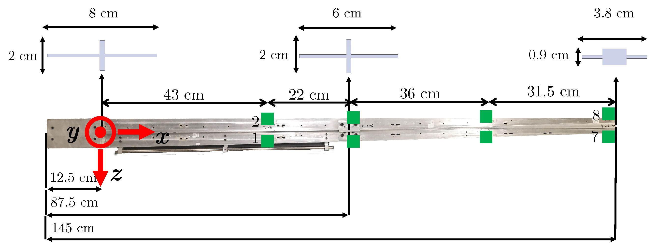The aerodynamic surface, based on a NACA 23015 airfoil, has a 1.5 m span (1.385 m from the reference origin in Figure 1), a mean aerodynamic chord of 0.172 m, a taper ratio of 0.35, and a leading-edge sweep of 1.49º. The wing torque box is formed by the spar and the tube. The spar, the focus of this work, is machined from two 6082-T6 aluminium blocks, welded together and reinforced using four bolted L-profile plates, and has a mass of 1.225 kg. Its cross-section is in the shape of a Saint George’s cross, and it tapers along the span. Its geometrical and cross-sectional characteristics are shown—with the stiffening tube installed—in Figure 1, alongside the accelerometer positioning.

The experimental data used in this work is retrieved from [6] (the experimental data and benchmark data can be retrieved from https://doi.org/10.17862/cranfield.rd.19077023, accessed on 1 September 2025), which also provides the benchmark EMA results. The spar was excited with a bandwidth-limited random input signal (2–400 Hz) at 0.305 g RMS amplitude, lasting 20 min. This input was applied via a Data Physics Signal Force™ modal shaker (Riverside, CA, USA) controlled by DP760™closed-loop control software. As shown in Figure 1, the accelerometers are placed in a 4-by-2 grid to record vertical acceleration, thus allowing the recording of transverse (i.e., flapwise) and torsional (i.e., pitching) vibrations. The data are recorded at a sampling frequency $f_s=$ 5120 Hz via a National Instruments cDAQ-9178, saving the data via a dedicated LabVIEW programme, developed in-house (at Cranfield University). 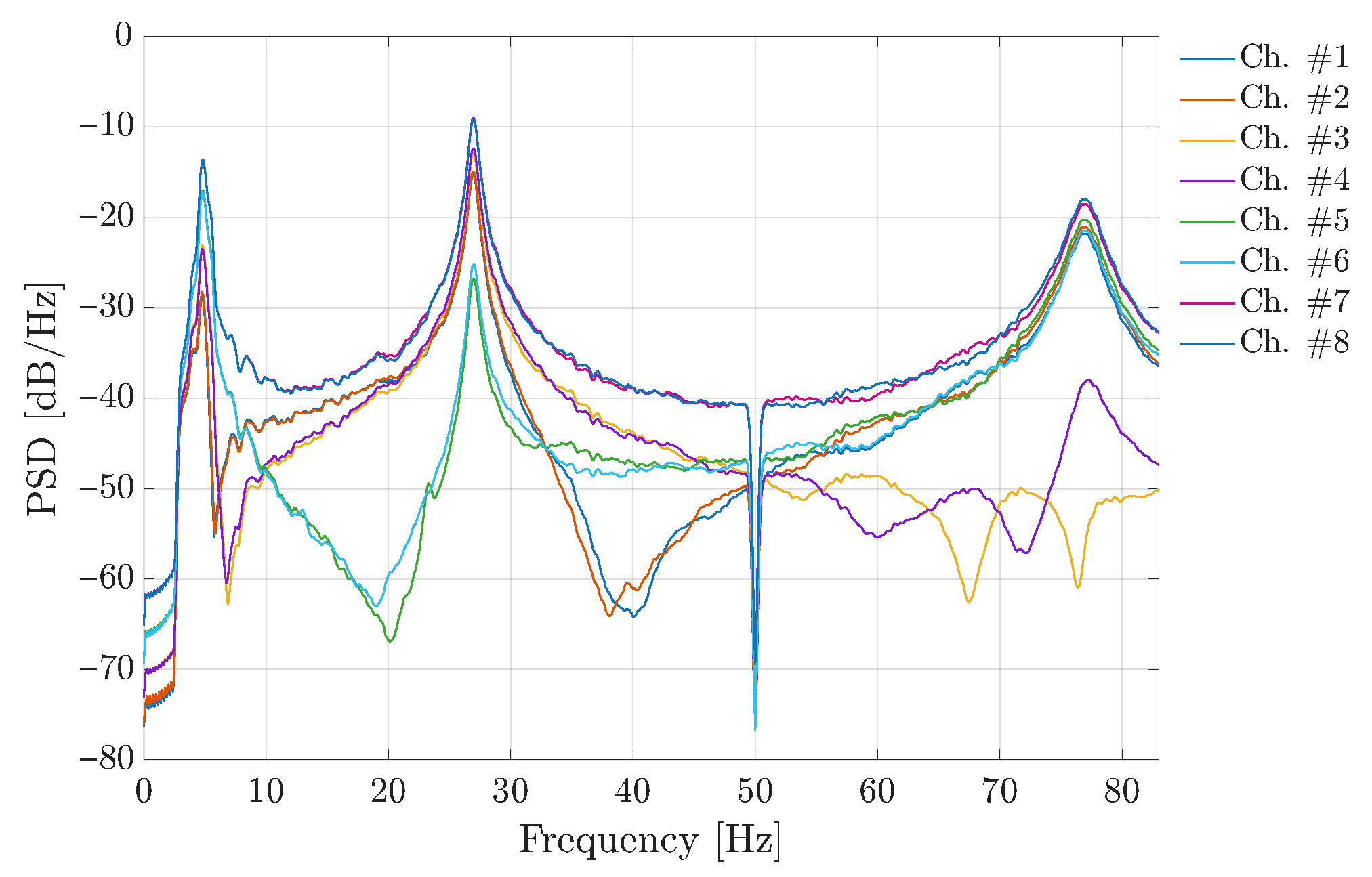Then, the acceleration time series are converted into ms⁻² and are bandpass-filtered between 3.25 and 85 Hz—to exclude drifts at low frequencies—and bandstop-filtered between 49.5 and 50.5 Hz to exclude electricity mains-induced drift (in the UK, the mains electricity AC frequency is 50 Hz). The upper bound of the passband filter is set to 85 Hz, as all modes of interest lie below this frequency. Considering the eight output channel time series, it is possible to obtain the response spectra, in the form of power spectral density (PSD). This is achieved via the built-in MATLAB pwelch function (https://uk.mathworks.com/help/signal/ref/pwelch.html, accessed on 1 September 2025). Figure 2 shows the PSD for the signals under scrutiny, given a number of discrete Fourier transform points of 2048 with 256 samples overlapping and a Hamming window of length 1024 to smooth out the spectra.

From Figure 2, it is clear that three main peaks exist in the PSD, and these can also be directly ascribed to the three modes of interest, which are known to exist around 4.8, 27, and 76.8 Hz. Please note that the dip at around 50 Hz in the PSD is to be attributed to the bandstop filter. Furthermore, the resonance-like peak and anti-resonance-like shapes (respectively, in channels #3 and 4) are due to local interaction with the spar reinforcement plates, to which the accelerometers are attached, and not to global system dynamics. In fact, these do not appear in the PSDs of the remaining channels or in any FRF. The latter are not shown for brevity’s sake, but can be seen in the benchmark work [6].

After this, the identification process can start by feeding all eight output acceleration time series into NExT to obtain IRFs discretised over 2048 points. It should be noted that this work only considers the acceleration time series retrieved from accelerometer #8 (as shown in Figure 1) as a reference channel for the NExT algorithm, as it is observed that the NExT-derived FRFs using accelerometer #8 as the reference (figure not included for brevity) more clearly show the three expected peaks. Then, the FFT of the IRFs (defined in the time domain) is computed to obtain the FRF (in the frequency domain) of the system, also discretised over 2048 points. This is then fed into the LF to obtain the system modal parameters. For NExT-ERA, instead of obtaining the FRFs, the IRFs are fed directly into the ERA algorithm for modal parameter extraction. Concerning SSI, the acceleration time series are directly fed into the algorithm for obtaining the modal parameters. In order to exclude outliers and spurious modes, the modal identifications are carried out over a range of model orders k, such that $k\in$ [6; 50], and stabilisation diagrams are used to identify the stable modes. The model order k was selected such that the methods would show a consistent number of stable modes—this could not be achieved for ERA, as discussed later. The ${\omega }_n$ range considered is between 0 and 83 Hz for a stability parameter of 0.5 %, and the range of ${\zeta }_n$ is 0.01-0.03 with a stability parameter of 5%. The stability parameter is satisfied after five consecutive identifications. 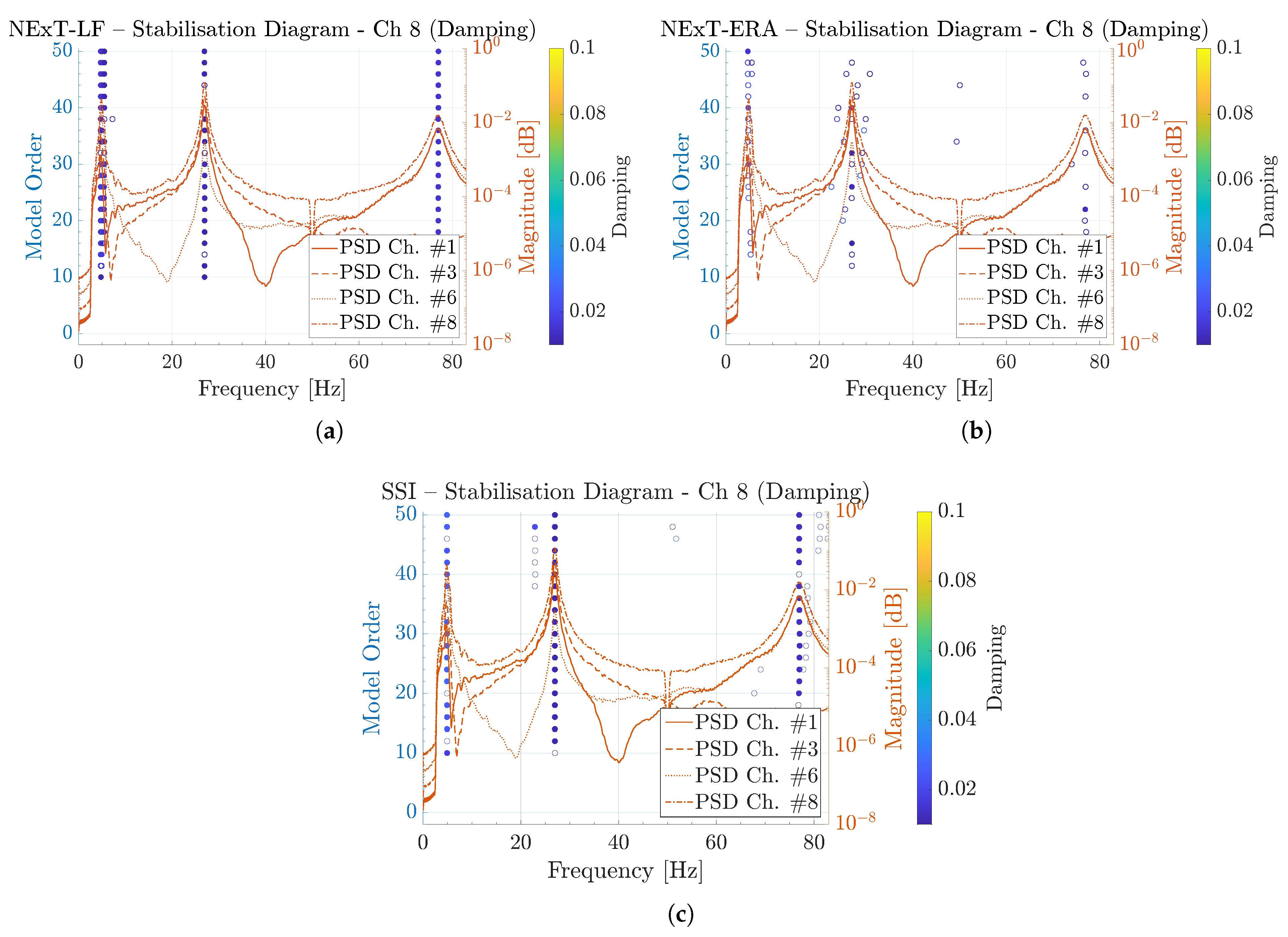This includes a stability requirement for ${\mathit{\varphi }}_n$, such that the Modal Assurance Criterion (MAC) number within the identified modes is equal to or larger than 0.95. The stabilisation diagram for the identifications carried out via NExT-LF, NExT-ERA, and SSI are shown in Figure 3.

It is clear from Figure 3 that the NExT-LF and SSI identifications are much more stable—particularly in ${\zeta }_n$—than the NExT-ERA counterpart. In fact, the latter shows essentially no stable modes in damping. This is confirmed by the identified ${\omega }_n$ and ${\zeta }_n$ results presented in

Table 1. Natural frequencies identified from the XB-2 main spar.

Natural Frequency [Hz] (Difference w.r.t. to Benchmark [%])
Mode #	Benchmark [6]	NExT-LF	NExT-ERA	SSI
1	4.855	4.930	4.689	4.891
	(-)	(1.53)	(−3.42)	(0.73)
2	26.966	26.922	26.942	26.969
	(-)	(−0.16)	(−0.09)	(0.01)
3	76.851	77.011	76.923	76.940
	(-)	(0.21)	(0.09)	(0.12)

and

Table 2. Modal damping ratios identified from the XB-2 main spar.

Modal Damping Ratios [-] (Difference w.r.t. to Benchmark [%])
Mode #	Benchmark [6]	NExT-LF	NExT-ERA	SSI
1	0.033	0.016	0.015	0.027
	(-)	(−51.17)	(−53.00)	(−17.01)
2	0.010	0.011	0.012	0.011
	(-)	(7.29)	(11.40)	(3.06)
3	0.014	0.015	0.013	0.014
	(-)	(7.35)	(−7.46)	(−3.17)

, respectively.

The ${\omega }_n$ identified from NExT-LF, NExT-ERA, and SSI are all coherent (maximum error of −3.42% for ${\omega }_1$ from NExT-ERA) with the benchmark results from [6]. However, a greater deviation is shown in Table 2 for ${\zeta }_n$. In particular, the absolute error for the ${\zeta }_1$ identification exceeds 50% for NExT-LF and NExT-ERA—although the NExT-LF error is lower than that of NExT-ERA—and that of SSI is around 17%. For ${\zeta }_{1-2}$, the NExT-LF-identified values show a deviation, always in absolute terms, around 7.3%, while those from NExT-ERA are higher, at 11.4% and 7.46%, for ${\zeta }_{1-2}$ respectively. On the other hand, the SSI identification results for ${\zeta }_s$ are the most coherent with the benchmark identification, although the ${\zeta }_1$ absolute error is over 17%.

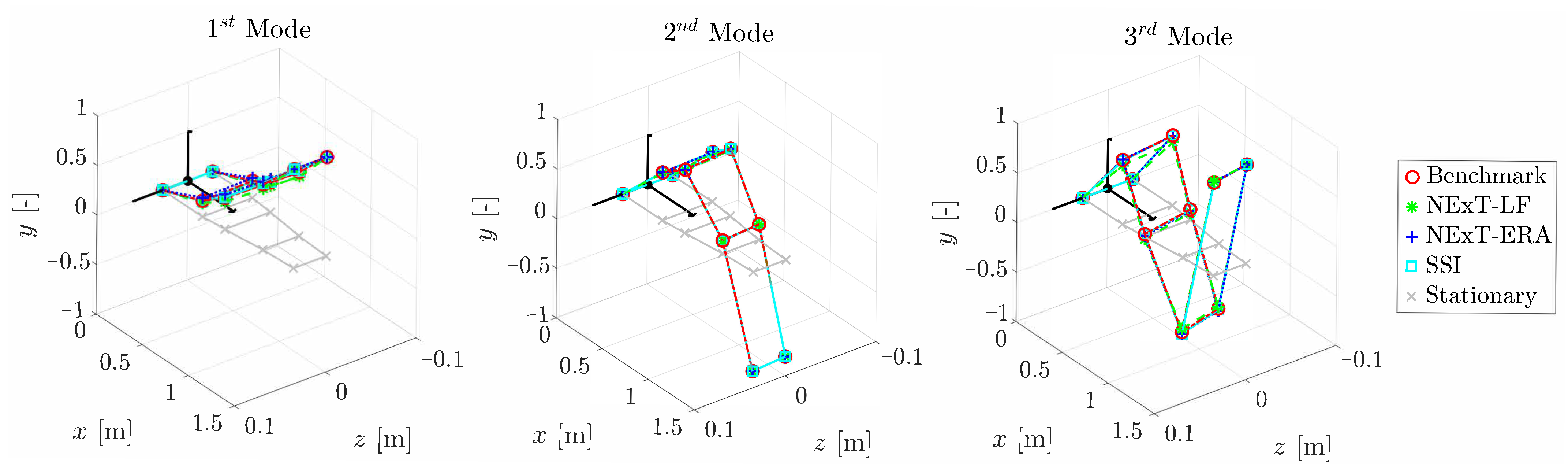
Having discussed the ${\omega }_n$ and ${\zeta }_n$ identifications, the ${\mathit{\varphi }}_n$ identification results need to be discussed. As per the ${\omega }_n$, all ${\mathit{\varphi }}_n$ identified from output-only data are coherent with the benchmark counterpart, yielding a MAC (diagonal) value of, or close to, 1. Figure 4 shows the ${\mathit{\varphi }}_n$ obtained from the output-only identification via NExT-LF, NExT-ERA, and SSI superimposed on the benchmark results in [6]. As already mentioned, these perfectly match the benchmark result.

In summary, it can be said that NExT-LF performs better than the well-known NExT-ERA for modal identification from output-only data. In addition, the NExT-LF is much more stable across different model orders, as shown in Figure 3. Nevertheless, a similar level of stability is shown by SSI, which is more precise than NExT-LF in terms of ${\zeta }_n$ identification. Nevertheless, this experimental dataset shows well-separated (in frequency) modes only in a lower-order system, which is an ideal scenario for SSI. As previously demonstrated in [11] for a full aircraft under multi-input multi-output testing conditions, SSI-based techniques (either input–output, such as N4SID, or the same output-only implementation used here) struggle in higher-order (many channels) systems, while input–output LF is much more robust. Further validation on this point is foreseen in future work on the NExT-LF to confirm its robustness for large systems with close-in-frequency modes.

4. Conclusions

This work briefly presented the first application of a recently introduced output-only variant of the Loewner Framework (LF), based on the Natural Excitation Technique (NExT), to an aeronautically relevant structure for operational (i.e., output-only) modal analysis. The results indicate that the modal parameters extracted using NExT-LF align well with experimental benchmark values. The proposed NExT-LF approach also demonstrated greater stability than NExT with the Eigensystem Realisation Algorithm (NExT-ERA), particularly in identifying natural frequencies. While the estimated values of the damping ratios exhibited some deviation, NExT-LF remained more reliable than NExT-ERA, although the Stochastic Subspace Identification (SSI) technique still outperforms both. Despite SSI providing better precision in damping identification, it is known to struggle with high-order systems and closely spaced modes. Hence, further work will be required on large structures with closely spaced modes to fully validate the potential advantages of NExT-LF in such scenarios.