PM_2.5 Concentration Estimation Based on Support Vector Regression: Hybrid Approach Using PM_2.5-Sensitive Pixels and Multi-Features ^†

Abstract

Fine particulate matter (${\mathrm{P}\mathrm{M}}_{2.5}$) is a hazardous air pollutant that poses serious risks to human health. Long-term exposure to high concentrations of ${\mathrm{P}\mathrm{M}}_{2.5}$ increases the likelihood of developing cardiovascular and respiratory diseases. Therefore, accurately monitoring ${\mathrm{P}\mathrm{M}}_{2.5}$ concentrations are crucial for effective air quality management. However, due to the limited number and uneven distribution of monitoring stations, traditional monitoring methods fail to provide comprehensive data. With advancements in imaging technology and data processing, researchers have focused on estimating ${\mathrm{P}\mathrm{M}}_{2.5}$ concentrations using image-based approaches. We constructed the ${\mathrm{P}\mathrm{M}}_{2.5}$-sensitive pixel (PSP) approach. In addition to the original four image features—Sobel, Dark Channel Prior (DCP), entropy, and contrast—we identified a new image feature and integrate three meteorological variables, relative humidity, temperature, and wind speed, to enhance the estimation of ${\mathrm{P}\mathrm{M}}_{2.5}$ concentrations.

1. Introduction

Air pollution has become an increasingly serious issue, attracting global attention as both an environmental and public health concern. Among various pollutants, fine particulate matter (PM_2.5) poses significant health risks due to its extremely small particle size, which allows it to remain suspended in the atmosphere for extended periods and penetrate deep into the human respiratory system, eventually reaching the bloodstream [1]. Its effects are particularly evident on the cardiovascular, cerebrovascular, and respiratory systems [2]. According to data released by the World Health Organization (WHO), approximately 4.2 million premature deaths occur each year due to prolonged exposure to outdoor PM_2.5 pollution, underscoring the serious threat this pollutant poses to human health [2].

In Taiwan, PM_2.5 is also one of the major contributors to poor air quality. According to the 12th edition of the Taiwan Emission Data System (TEDS 12.0) published by the Environmental Protection Administration, the primary sources of PM_2.5 emissions originate from various anthropogenic activities. The most significant contributors include road dust, emissions from construction sites, vehicular exhaust, and industrial processes, accounting for approximately 41%, 23%, and 22% of total emissions, respectively [3]. This affects the quality of urban life and causes severe damage to the overall environment.

2. Related Work

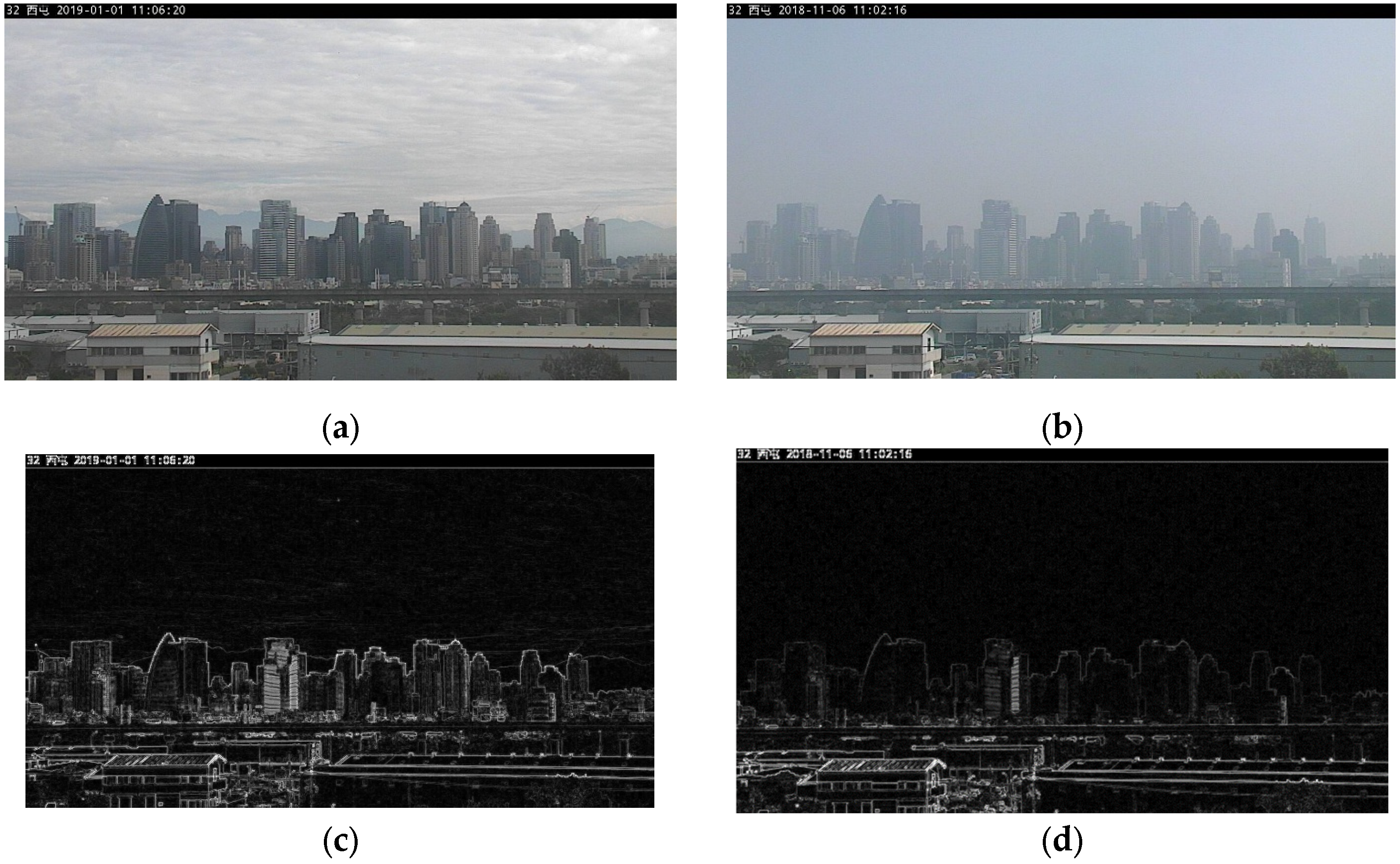
Traditional image analysis methods using high-pass filtering are commonly employed to emphasize high-frequency information in images [4], thereby highlighting the contours of buildings to estimate ${\mathrm{P}\mathrm{M}}_{2.5}$ concentrations in the air (Figure 1). The experiment demonstrates that in the low-concentration image (a), the building contours become clearly identifiable after applying the high-pass filter (c). In contrast, the high-concentration image (b), when processed similarly (d), appears blurred, with indistinct contour edges. This phenomenon reflects the impact of air pollution on image details and can serve as a reference for estimating ${\mathrm{P}\mathrm{M}}_{2.5}$ concentration levels.

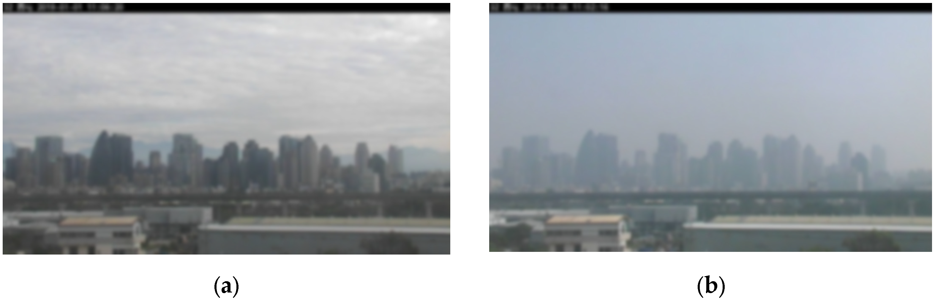
We explored whether low-pass filtering can similarly reflect variations in ${\mathrm{P}\mathrm{M}}_{2.5}$ concentrations. Low-pass filtering primarily preserves the low-frequency information in an image. For low-pollution images with clear visual features, the difference between the original image and the low-pass filtered result (a) is more pronounced (Figure 2). In contrast, for high-pollution images that are already hazy, the difference between the original and the filtered image (b) is relatively minimal. This distinction may assist in identifying changes in air quality and offers an alternative approach to image-based air pollution assessment.

3. ${\mathbf{P}\mathbf{M}}_{2.5}$ Concentration Estimation

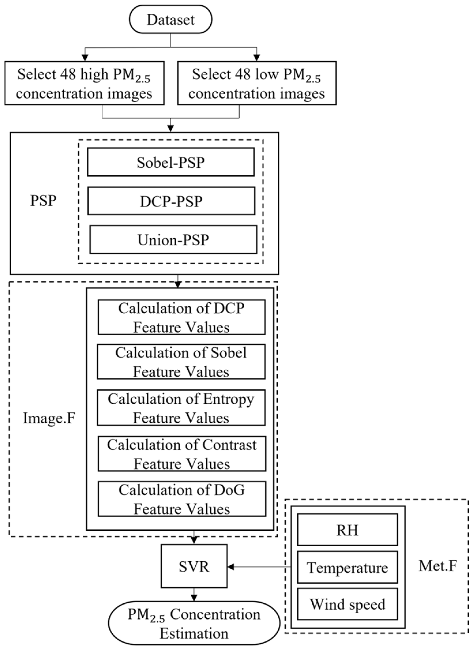
We adopted the ${\mathrm{P}\mathrm{M}}_{2.5}$-sensitive pixels (PSP) method to identify regions that exhibit strong responses to variations in ${\mathrm{P}\mathrm{M}}_{2.5}$ concentration [5]. A total of 48 images, representing high and low ${\mathrm{P}\mathrm{M}}_{2.5}$ concentration levels were processed using either the Sobel filter or the dark channel prior (DCP) method (Figure 3). The resulting images are then subtracted (low–high ${\mathrm{P}\mathrm{M}}_{2.5}$) to highlight the differential regions. These sensitive regions are aggregated and normalized to generate the PSP image, from which air quality-related image features are extracted. The extracted features include DCP, Sobel, entropy, contrast, and difference of Gaussian (DoG). DoG is the additional feature employed in this study. The resulting feature values are then fed into a support vector regression (SVR) model to estimate ${\mathrm{P}\mathrm{M}}_{2.5}$ concentrations.

3.1. Image Features

To estimate PM_2.5 concentrations in the atmosphere, we extracted image features related to air pollution from monitoring station imagery, including Sobel, DCP, entropy, DoG, and contrast.

3.1.1. Sobel

The object contours are highlighted by calculating the intensity gradient of each pixel in the horizontal and vertical directions [6]. Two 3 × 3 convolution kernels are applied separately in the horizontal direction (G_x) and the vertical direction (G_γ) to extract edge information from the image. The kernel formats are as follows.

$$G_x=\left[\begin{array}{ccc}-1& 0& 1\\ -2& 0& 2\\ -1& 0& 1\end{array}\right],$$

(1)

$$G_y=\left[\begin{array}{ccc}1& 2& 1\\ 0& 0& 0\\ -1& -2& -1\end{array}\right],$$

(2)

Total gradient calculation is conducted using Equation (3).

$$G\left(i,j\right)={|G}_x\left(i,j\right)|+\left|G_y\left(i,j\right)\right|,$$

(3)

Here, $G\left(i,j\right)$ represents the overall gradient magnitude at position $\left(i,j\right)$ in the image, where $G_x\left(i,j\right)$ and $G_y\left(i,j\right)$ denote the horizontal and vertical gradient components, respectively.

3.1.2. DCP

DCP is widely used in the image dehazing method. Its core concept is based on the observation that, in natural (non-synthetic) images, excluding sky regions, at least one color channel (red, green, or blue) typically contains pixels with very low intensity values (close to zero) [7]. This phenomenon often occurs in areas with shadows or object boundaries, making it a useful feature for assessing image blurriness.

$$J^{dark}(x,y)=\underset{c\in \{r,g,b\}}{\min }\left(\underset{y\in \mathsf{\Omega }\left(x\right)}{\min }{J}^c\left(y\right)\right),$$

(4)

Here, $J^{dark}(x,y)$ denotes the dark channel value at position $(x,y)$, where $c\in \{r,g,b\}$ represents the red, green, and blue channels, and $y\in \mathsf{\Omega }\left(x\right)$ indicates a local patch centered at pixel $x$. $J^c\left(y\right)$ is the intensity value at position $y$ in channel $c$. The computation first selects the minimum intensity among the R, G, and B channels for each pixel, and then identifies the lowest intensity within the local patch to output as the dark channel value at that location.

3.1.3. Entropy

Entropy is used to measure the uncertainty and complexity of data. A higher entropy value indicates greater diversity and unpredictability (typically associated with lower PM_2.5 concentrations) [8], while a lower entropy value suggests more uniform and less variable data (often corresponding to higher PM_2.5 concentrations).

$$H=-\sum _{i=0}^L{p}_i{log}_2\left(p_i\right),$$

(5)

Here, $H$ denotes the total entropy of the image, $L$ represents the total number of grayscale levels (typically 255), and $p_i$ is the probability distribution of grayscale level $i$ across the entire image. When the distribution of grayscale values is concentrated around a small number of levels, the image entropy decreases, indicating less variation within the image. Conversely, if the grayscale values are evenly distributed, the entropy value becomes higher, reflecting greater image complexity.

3.1.4. Contrast

Contrast is used to measure variations in pixel brightness, reflecting the degree of change between illuminated and shadowed areas within an image. High-contrast images typically exhibit clearer contours and finer details, whereas low-contrast images tend to appear blurred or hazy. This feature is widely used not only for image quality assessment [9] but also as a key indicator for analyzing atmospheric visibility. The equation is as follows:

$$C=\sqrt{{\displaystyle \frac{1}{N}}\sum _{i=1}^N{(I_i-\mu )}^2},$$

(6)

Here, $C$ denotes the contrast value of the entire image, $N$ represents the total number of pixels, i is the grayscale intensity of the i-th pixel, and $\mu$ is the mean grayscale value of the image. This formula calculates the standard deviation of image brightness, which describes the degree of variation between bright and dark regions. A larger standard deviation indicates more pronounced differences in brightness and thus higher contrast, while a standard deviation close to zero suggests uniform brightness across most areas of the image, resulting in a more blurred appearance.

3.1.5. DoG

DoG is used to extract image features by subtracting two Gaussian-blurred images with different standard deviations [10].

$$DoG\left(x,y\right)=G\left(x,y,{\sigma }_1\right)-G\left(x,y,{\sigma }_2\right),$$

(7)

Here, $DoG\left(x,y\right)$ represents the difference between two Gaussian-blurred images. $G\left(x,y,{\sigma }_1\right)$ denotes the result of applying Gaussian filtering with standard deviation ${\sigma }_1$ to the original image, where $\left(x,y\right)$ is the pixel position and $\sigma$ is the standard deviation of the Gaussian kernel. A smaller ${\sigma }_1$ results in less blur, while a larger ${\sigma }_2$ in $G\left(x,y,{\sigma }_2\right)$ produces a more heavily blurred image.

3.2. Meteorological Features

Meteorological features play a critical role in the variation of ${\mathrm{P}\mathrm{M}}_{2.5}$ concentrations. In addition to influencing the transport and dispersion of particulate matter, they may also promote or inhibit the formation and transformation of particulate pollutants.

3.2.1. Relative Humidity

Relative humidity represents the ratio of the actual amount of water vapor in the air to the maximum amount the air can hold at a given temperature, expressed as a percentage [11]. This meteorological feature is highly correlated with ${\mathrm{P}\mathrm{M}}_{2.5}$ concentration levels. As humidity increases, moisture tends to adhere to the surface of suspended particles, causing them to expand in volume and increase in mass, which in turn affects visibility and image clarity. Under certain conditions, high humidity accelerates particle deposition, thereby reducing ambient ${\mathrm{P}\mathrm{M}}_{2.5}$ concentrations [12]. Therefore, incorporating relative humidity as one of the features in image-based estimation models can help improve both the accuracy and stability of predictions.

3.2.2. Temperature

Temperature is one of the key meteorological factors influencing atmospheric dispersion and particulate formation. Higher temperatures promote atmospheric convection, facilitating the vertical dispersion of pollutants and thereby reducing ${\mathrm{P}\mathrm{M}}_{2.5}$ concentrations near the surface. In contrast, lower temperatures weaken convective activity, leading to the accumulation of pollutants close to the ground [13]. Additionally, temperature affects the transformation rates of gaseous pollutants. Under high-temperature conditions, the conversion of sulfur dioxide and nitrogen oxides into sulfate and nitrate particles is accelerated, which can further increase ${\mathrm{P}\mathrm{M}}_{2.5}$ concentrations [14]. Therefore, incorporating temperature into the estimation model enhances its adaptability under varying climatic conditions.

3.2.3. Wind Speed

Wind speed is a critical meteorological factor that influences the dispersion and transport of air pollutants. Increased wind speed facilitates both horizontal and vertical diffusion of pollutants, helping to reduce ${\mathrm{P}\mathrm{M}}_{2.5}$ concentrations in certain areas. Conversely, low wind speed tends to hinder dispersion, leading to the accumulation of suspended particles and elevated ${\mathrm{P}\mathrm{M}}_{2.5}$ levels [13]. Moreover, under specific seasonal and topographic conditions, strong winds carry pollutants from other regions, resulting in short-term spikes in local concentrations. Thus, wind speed not only affects the efficiency of pollutant dilution but also reflects the impact of atmospheric movement on spatial concentration patterns. Incorporating wind speed into the model enhances its predictive capability.

4. Experiments

Results of different PSP feature extraction methods, Sobel, DCP, and a combined method, were compared across different geographic regions. Model performance was evaluated using root mean square error (RMSE) and the coefficient of determination (R²) as assessment metrics. We examined how different feature combinations and PSP extraction techniques affect the accuracy of ${\mathrm{P}\mathrm{M}}_{2.5}$ concentration predictions.

4.1. Dataset

We utilized image and meteorological data from the Xitun Air Quality Monitoring Station. The images were obtained from the Environmental Data Open Platform provided by the Ministry of Environment [15]. The data covers the period from August 2018 to September 2019, with six images captured per hour between 07:00 and 17:00 each day. Each image is paired with the corresponding hourly ${\mathrm{P}\mathrm{M}}_{2.5}$ concentration value and three meteorological variables—relative humidity, temperature, and wind speed—serving as inputs for model training and testing.

4.2. Evaluation Metrics

To evaluate the performance of the model in estimating ${\mathrm{P}\mathrm{M}}_{2.5}$ concentrations, $R^2$ and RMSE were used. $R^2$ is used to measure the accuracy of the predictions, while RMSE quantifies the magnitude of estimation errors.

4.2.1. R²

R² is used to assess how well a model’s predicted results align with actual observed data. Its value ranges from 0 to 1, where an R² closer to 1 indicates higher predictive accuracy, while an R² approaching 0 reflects poor predictive performance. R² is calculated as follows.

$$R^2=1-{\displaystyle \frac{{\sum }_{i=1}^n{\left(y_i-{\widehat{y}}_i\right)}^2}{{\sum }_{i=1}^n{\left(y_i-\widehat{y}\right)}^2}},$$

(8)

Here, $n$ is the number of data samples, $y_i$ is the actual value, ${\widehat{y}}_i$ is the predicted value from the model, and $\widehat{y}$ is the mean of the actual values. The numerator represents the residual sum of squares (RSS), while the denominator denotes the total sum of squares (TSS).

4.2.2. RMSE

RMSE is used for evaluating the magnitude of errors between predicted and actual values [16]. It is calculated by squaring the prediction errors for all data points, taking their average, and then computing the square root. This metric provides a measure of how far the predicted values deviate from the true values. RMSE is calculated as follows.

$$RMSE=\sqrt{{\displaystyle \frac{1}{n}}\sum _{i=1}^n{(y_i-{\widehat{y}}_i)}^2},$$

(9)

Here, $n$ is the number of data points, $y_i$ is the actual value of the i-th data sample, and ${\widehat{y}}_i$ is the predicted value produced by the model. A smaller RMSE value indicates a smaller difference between the predicted and actual values, signifying better predictive performance.

4.3. Comparison of Estimation Results

To investigate the impact of image features and PSP extraction methods on ${\mathrm{P}\mathrm{M}}_{2.5}$ concentration estimation. We experimented with the data from the Xitun Monitoring Station.

Table 1. Estimation performance comparison using single image features. (✓indicates that the corresponding feature is included.).

Experiment	Meteorological Feature	Sobel	DCP	Entropy	Contrast	DoG	Model	${\mathit{R}}^2$	RMSE
1	✓	✓					Sobel–PSP	0.9296	3.5209
	✓	✓					DCP–PSP	0.9521	3.6767
	✓	✓					Union–PSP	0.9519	3.6451
2	✓		✓				Sobel–PSP	0.9364	3.3557
	✓		✓				DCP–PSP	0.9543	3.6304
	✓		✓				Union–PSP	0.9533	3.6264
3	✓			✓			Sobel–PSP	0.9017	4.0948
	✓			✓			DCP–PSP	0.9170	4.8330
	✓			✓			Union–PSP	0.9176	4.8198
4	✓				✓		Sobel–PSP	0.9224	3.6383
	✓				✓		DCP–PSP	0.8845	5.6421
	✓				✓		Union–PSP	0.8800	5.8257
5	✓					✓	Sobel–PSP	0.9308	3.5047
	✓					✓	DCP–PSP	0.9526	3.6836
	✓					✓	Union–PSP	0.9515	3.6756

and

Table 2. Estimation performance comparison using multiple image features. (✓indicates that the corresponding feature is included.).

Exp	Meteorological Feature	Sobel	DCP	DoG	Model	${\mathit{R}}^2$	RMSE
1	✓	✓	✓		Sobel–PSP	0.9377	3.2671
	✓	✓	✓		DCP–PSP	0.9619	3.3336
	✓	✓	✓		Union–PSP	0.9631	3.2604
2	✓	✓		✓	Sobel–PSP	0.9254	3.5733
	✓	✓		✓	DCP–PSP	0.9571	3.4763
	✓	✓		✓	Union–PSP	0.9562	3.5144
3	✓		✓	✓	Sobel–PSP	0.9414	3.2649
	✓		✓	✓	DCP–PSP	0.9605	3.3619
	✓		✓	✓	Union–PSP	0.9616	3.3410
4		✓	✓	✓	Sobel–PSP	0.9302	3.4756
		✓	✓	✓	DCP–PSP	0.9600	3.3921
		✓	✓	✓	Union–PSP	0.9621	3.3485

show the results.

5. Conclusions

We estimate PM_2.5 concentrations by combining image features with meteorological variables based on the PM_2.5-sensitive pixel (PSP) approach. Five image features, Sobel, DCP, entropy, contrast, and DoG, were evaluated under three PSP extraction methods: Sobel–PSP, DCP–PSP, and Union–PSP. Among the single-feature experiments, DCP and DoG showed accurate estimation capabilities, while the combination of multiple features using the union–PSP method achieved the highest overall accuracy. This highlights the importance of integrating diverse feature types to enhance the robustness and adaptability of air pollution estimation models. The results provide a basis for the development of cost-effective, image-based air quality monitoring systems.

References

1. World Health Organization. Billions of People Still Breathe Unhealthy Air: New WHO Data. Available online: https://www.who.int/zh/news/item/04-04-2022-billions-of-people-still-breathe-unhealthy-air-new-who-data (accessed on 20 May 2025).
2. World Health Organization. Ambient (Outdoor) Air Pollution. Available online: https://www.who.int/news-room/fact-sheets/detail/ambient-(outdoor)-air-quality-and-health (accessed on 20 May 2025).
3. Su, S.Y.; Liaw, Y.P.; Jhuang, J.R.; Hsu, S.Y.; Chiang, C.J.; Yang, Y.W.; Lee, W.C. Associations between ambient air pollution and cancer incidence in Taiwan: An ecological study of geographical variations. BMC Public Health 2019, 19, 1496. [Google Scholar] [CrossRef] [PubMed]
4. Lin, D.-C. Estimation of Urban PM2.5 Concentration Based on Digital Image Processing Technology. Master’s Thesis, Department of Information and Communication, Chaoyang University of Technology, Taichung, Taiwan, 2019. Available online: https://www.airitilibrary.com/Article/Detail/U0078-0510202013412581 (accessed on 10 April 2025).
5. Jiang, M.-Y. Using PM2.5-Sensitive Pixels Combined with Weather Features to Improve the Estimation Performance of PM2.5 Concentration in Cities. Master’s Thesis, Department of Information and Communication, Chaoyang University of Technology, Taichung, Taiwan, July 2022. Available online: https://ir.lib.cyut.edu.tw/bitstream/310901800/41262/1/110CYUT0652013-002.pdf (accessed on 10 April 2025).
6. Gonzalez, R.C.; Woods, R.E. Digital Image Processing, 4th ed.; Pearson: London, UK, 2018. [Google Scholar]
7. He, K.; Sun, J.; Tang, X. Single image haze removal using dark channel prior. In Proceedings of the 2009 IEEE Conference on Computer Vision and Pattern Recognition, Miami, FL, USA, 20–25 June 2009; pp. 1956–1963. [Google Scholar]
8. Shannon, C.E. A mathematical theory of communication. Bell Syst. Tech. J. 1948, 27, 379–423. [Google Scholar] [CrossRef]
9. Gu, K.; Zhai, G.; Lin, W.; Liu, M. The analysis of image contrast: From quality assessment to automatic enhancement. IEEE Trans. Cybern. 2015, 46, 284–297. [Google Scholar] [CrossRef] [PubMed]
10. Marr, D.; Hildreth, E. Theory of edge detection. Proc. R. Soc. Lond. Ser. B Biol. Sci. 1980, 207, 187–217. [Google Scholar] [CrossRef] [PubMed]
11. Wang, J.; Ogawa, S. Effects of meteorological conditions on PM2.5 concentrations in Nagasaki, Japan. Int. J. Environ. Res. Public Health 2015, 12, 9089–9101. [Google Scholar] [CrossRef] [PubMed]
12. Swietlicki, E.; Zhou, J.; Berg, O.H.; Martinsson, B.G.; Frank, G.; Cederfelt, S.I.; Dusek, U.; Berner, A.; Birmili, W.; Wiedensohler, A.; et al. A closure study of sub-micrometer aerosol particle hygroscopic behavior. Atmos. Res. 1999, 50, 205–240. [Google Scholar] [CrossRef]
13. Zhang, H.; Wang, Y.; Hu, J.; Ying, Q.; Hu, X.-M. Relationships between meteorological parameters and criteria air pollutants in three megacities in China. Environ. Res. 2015, 140, 242–254. [Google Scholar] [CrossRef] [PubMed]
14. Jacob, D.J.; Winner, D.A. Effect of climate change on air quality. Atmos. Environ. 2009, 43, 51–63. [Google Scholar] [CrossRef]
15. Environmental Protection Administration. Open Environmental Data Platform. Available online: https://data.moenv.gov.tw/ (accessed on 20 May 2025).
16. Chicco, D.; Warrens, M.J.; Jurman, G. The coefficient of determination R-squared is more informative than SMAPE, MAE, MAPE, MSE and RMSE in regression analysis evaluation. PeerJ Comput. Sci. 2021, 7, e623. [Google Scholar] [CrossRef] [PubMed]
Figure 1. Images of high and low P M 2.5 concentrations and their high-pass filtered versions: (a) low P M 2.5 concentration image; (b) high P M 2.5 Concentration Image; (c) high-pass filtered image of low P M 2.5 concentration; (d) high-pass filtered image of high P M 2.5 concentration.
Engproc 120 00048 g001
Figure 2. Low-pass filtered images of high and low P M 2.5 concentrations: (a) low- P M 2.5 concentration low-pass filtered image; (b) high- P M 2.5 concentration low-pass filtered image.
Engproc 120 00048 g002
Figure 3. PSP process. The dashed boxes represent different functional modules in the proposed framework, including PSP extraction, image feature calculation, and meteorological feature integration.
Engproc 120 00048 g003