Noise Injection as a Structural Diagnostic Tool for Deep Model Reduction ^†

Abstract

In this study, we introduce a novel, functionally driven method for model pruning guided by sensitivity analysis. Conventional model compression techniques often rely on proxy metrics, such as weight magnitude, which may not accurately reflect a component’s true functional importance. The proposed method directly assesses this by systematically injecting controlled noise into network layers and measuring the resultant perturbation on inference output. Components exhibiting low sensitivity to this noise are identified as functionally redundant and are pruned. We validated the method on EEGNet, a compact convolutional neural network, using the MNE Sample Event-Related Potential (ERP) dataset, a widely used benchmark for electroencephalography classification. After training the baseline model, we generated a sensitivity profile by quantifying how noise injection at different layers impacts predictive accuracy. This profile then guided targeted pruning of less influential convolutional kernels and weights. Experimental results demonstrate the method’s efficacy, achieving a significant reduction in both parameter count and computational complexity. Crucially, the pruned model retains classification accuracy nearly identical to the original, heavyweight EEGNet. This confirms that sensitivity-guided pruning effectively removes redundancy without degrading performance. In conclusion, our noise injection framework provides a more direct and interpretable criterion for neural network simplification. By linking component pruning to functional impact, our method enables a more precise and efficient model reduction than traditional heuristic-based approaches. The method developed presents a practical pathway toward developing lightweight, accurate, and low-latency models essential for real-world neuro-computational applications. Future work will focus on automating the pruning pipeline and extending the framework’s applicability to diverse neural architectures.

1. Introduction

Simplifying deep learning models has become increasingly important for deploying AI systems in resource-constrained environments such as wearable devices, mobile applications, and edge computing platforms. These applications demand lightweight models that can function under strict limitations in memory, computation, and energy consumption, without significantly compromising accuracy. To address these constraints, researchers have proposed various simplification strategies that generally fall into two broad categories.

The first approach, model compression [1,2], focuses on reducing the internal complexity of neural networks while preserving predictive accuracy. Common techniques include structured pruning [3,4], quantization [5,6], knowledge distillation [7,8], and low-rank factorization [9,10]. These methods eliminate redundant parameters, lower numerical precision, or transfer knowledge from a larger network to a smaller one, thereby reducing parameter count, computation load, and storage requirements. The second approach, model reduction, targets simplification of the model’s overall architecture or functional representation. This strategy aims to speed up inference, enhance interpretability, or enable deployment on limited hardware. While it shares similar objectives with model compression, model reduction tends to involve more structural modifications to the network.

In this study, we introduce a novel model reduction technique that leverages noise injection during inference to guide the simplification process. By injecting controlled noise into various layers and analyzing its impact on output predictions, we infer the relative importance of each layer. The underlying hypothesis is that layers more tolerant to perturbations are less essential to the model’s final performance and are therefore suitable candidates for pruning or simplification. The method developed in this study is iterative and data-driven. By systematically perturbing layers and observing resulting changes in the output, we build a sensitivity profile that indicates the importance of each layer. This profile then informs decisions on which components can be reduced or removed with minimal effect on accuracy. While traditional pruning methods rely on heuristics, including weight magnitude or backpropagation gradients, the method directly ties layer importance to output robustness under perturbation, offering a more task-relevant reduction metric.

We evaluated the developed method on standard benchmarks in brain–computer interface (BCI) applications. Experimental results demonstrate that the method performs competitively with existing compression and reduction methods. More notably, we show that significant portions of the network can be removed with only minor degradation in output quality, confirming the effectiveness of noise-guided sensitivity analysis as a model reduction strategy.

2. Background Knowledge

In the previous study [11], we addressed the issue of high-dimensional electroencephalography (EEG) data in the BCI system by proposing a channel selection algorithm based on noise injection—localization and selection using training with noise injection (LSvT-NI). The high dimensionality of EEG data not only increases model size and computational complexity but also affects user comfort and system performance. Therefore, reducing the number of channels while maintaining classification accuracy is a critical challenge.

The core idea of LSvT-NI is that EEG channels containing essential features are more sensitive to noise. During training, the algorithm injects either white or pink noise into each EEG channel and observes the resulting degradation in classification accuracy to evaluate the importance of each channel. In each iteration, the channel that causes the most significant drop in performance is selected and added to a candidate set. This process continues until the model meets a predefined accuracy threshold. In this strategy, LSvT-NI effectively identifies the most critical channels for classification.

In the experiments, EEGNet [12] was used as the baseline model, and the BCI Competition IV 2a dataset was employed, which includes motor imagery EEG data from nine subjects across four classes, recorded using 22 channels. The model was evaluated under various signal-to-noise ratio (SNR) conditions (0, 5, 10, and 15 dB). Results show that under 5 dB white noise, LSvT-NI reduces the number of channels from 22 to 5 (a 77.3% reduction), while maintaining classification accuracy and reducing computational complexity (MACs) by 86.9%. Similar outcomes were observed with pink noise.

Compared to other channel selection methods—such as attention mechanisms or heuristic approaches—LSvT-NI achieves higher channel reduction and better efficiency, owing to its iterative training strategy based on noise sensitivity. LSvT-NI provides an effective EEG channel selection framework that significantly reduces input dimensionality and computation, making it highly suitable for wearable and edge AI BCI systems. Future work will explore its generalization capabilities across diverse datasets and subject-independent settings.

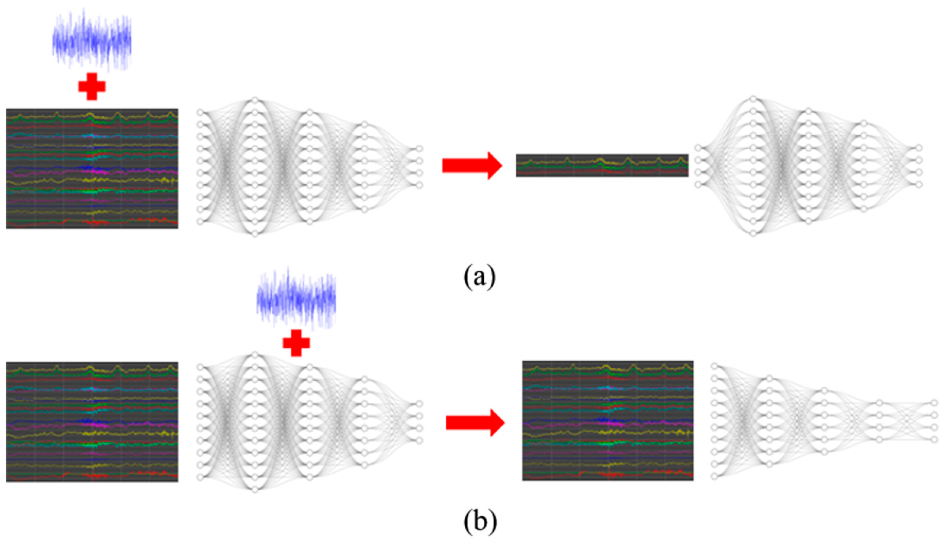
Such findings enable the extension of the use of noise injection beyond EEG channel reduction to explore its potential for simplifying the model architecture itself. Figure 1 illustrates the system concept of both the LSvT-NI algorithm and the developed method. In Figure 1a, noise is injected into the input EEG signals, and the LSvT-NI algorithm identifies and selects the most critical channels, allowing input dimensionality to be reduced without compromising classification accuracy. In Figure 1b, we inject noise into components of the EEGNet architecture and observe its impact to identify redundant structures and guide network simplification.

3. Method

EEGNet is a compact convolutional neural network (CNN) specifically designed for processing EEG data. Developed by Lawhern et al., EEGNet is notable for its low parameter count, strong interpretability, and broad applicability across various BCI paradigms [12]. The model integrates essential components of traditional EEG signal processing—namely, temporal filtering, spatial filtering, and feature integration—into a single end-to-end deep learning framework.

The EEGNet architecture comprises three computational blocks. The first block is the temporal convolutional layer (Conv2D), which performs 1D convolution along the time axis to simulate a bank of bandpass filters. This layer is governed by the hyperparameter F1, which specifies the number of temporal filters to be learned. For instance, setting F1 to 8 enables the model to learn eight distinct filters that can correspond to canonical EEG rhythms, such as alpha, beta, or gamma bands. These filters extract frequency-specific temporal patterns and offer physiologically meaningful representations commonly used in EEG analysis. The second block is the depthwise spatial convolutional layer (DepthwiseConv2D), which learns spatial features across EEG channels. In contrast to standard convolution, EEGNet applies D separate spatial filters per temporal filter output, where D is the depth multiplier hyperparameter. This configuration allows the network to explore diverse spatial configurations for each temporal feature. For example, with F1 = 8 and D = 2, the model produces 16 output feature maps (8 × 2), each reflecting a unique spatial projection across all EEG channels. This design supports the extraction of distinct spatial patterns associated with neural activity. The third block is the separable convolutional layer (SeparableConv2D), consisting of two operations: a depthwise temporal convolution and a pointwise (1 × 1) convolution. The former summarizes temporal information using a kernel size of 1 × 16, while the latter integrates information across feature maps. This two-step process enables expressive and computationally efficient feature extraction. Subsequent layers—including average pooling, batch normalization, and dropout—are used to reduce dimensionality, normalize activation statistics, and prevent overfitting, respectively.

Final classification is conducted using a fully connected (dense) layer followed by a softmax activation function. The input to the dense layer is determined by the number of feature maps (F1 × D) and the downsampled temporal length after pooling. For instance, with F1 = 64, D = 8, and T = 128 time points, assuming two pooling layers (each halving the temporal dimension), the final input to the dense layer would be a feature vector of size 512 × 4 = 2048.

Overall, EEGNet enables efficient and interpretable feature learning with a minimal number of parameters—typically ranging from several thousand to tens of thousands—making it well-suited for real-time and resource-constrained BCI applications, such as wearable EEG devices and edge AI systems. Its architectural simplicity and flexibility have led to widespread adoption in modern EEG-based deep learning research. 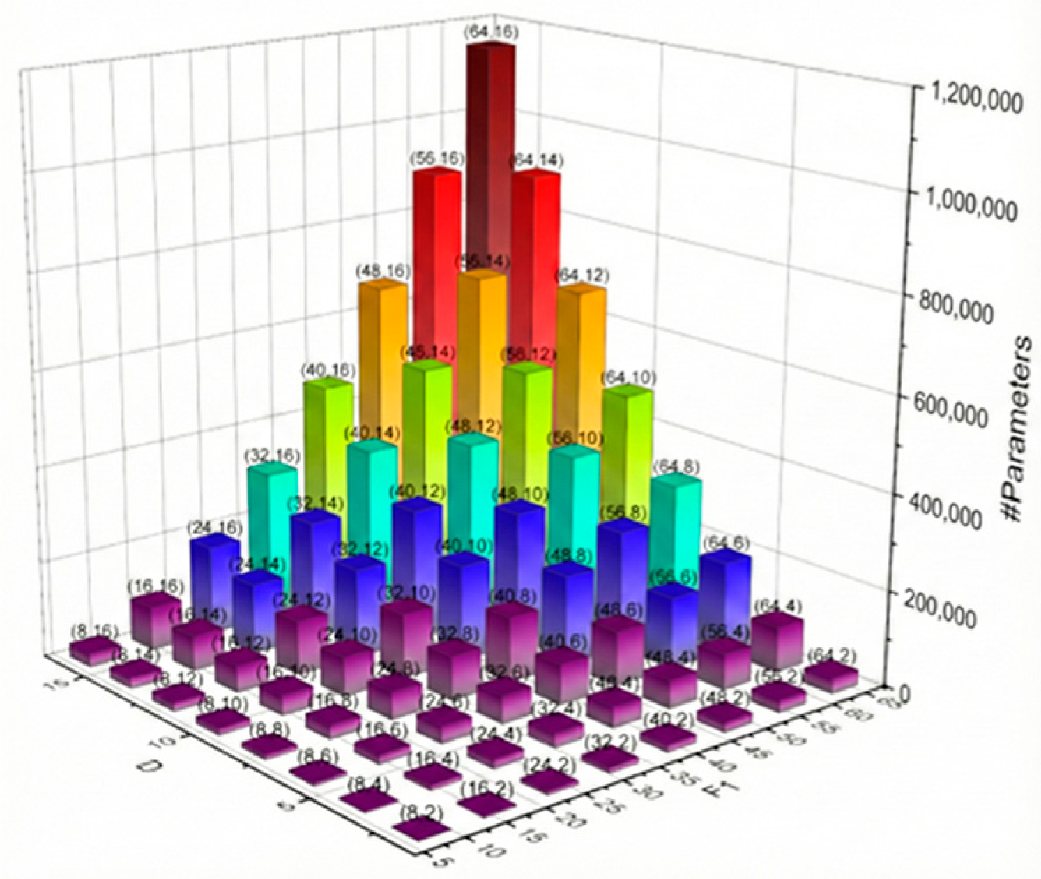Figure 2 illustrates the total number of trainable parameters in EEGNet under varying values of F1 (from 8 to 64) and D (from 2 to 16), highlighting the trade-off between model complexity and representational capacity.

We created the following algorithm (Algorithm 1) for reducing Conv2D temporal filters through noise injection.

Algorithm 1. A noise-injection–based filter importance analysis and model reduction procedure for EEGNet. The algorithm ranks temporal convolutional filters by their robustness to controlled noise perturbations, identifies a critical subset whose removal minimally degrades performance, and retrains a compact EEGNet with reduced filters while preserving classification accuracy

Step-1. Model Initialization ● Build and train EEGNet with F temporal filters and depth multiplier D. ● Record the baseline classification accuracy Abaseline. Step-2. Single Filter Noise Injection ● For each filter i in 0 to F − 1: ■ Replace the weights of filter i with white noise of SNR dB. ■ Evaluate the model and record the resulting accuracy Ai. Step-3. Filter Ranking ● Sort all F filters based on Ai in descending order. ● This produces a ranked list R, where filters that affect accuracy the least are ranked higher. Step-4. Progressive Noise Injection Analysis ● For each k from 1 to F: ■ Inject noise into the top-k filters in R. ■ Measure the new inference accuracy Ak. ● Find the critical value k* where Ak* drops below a desired threshold or begins to significantly degrade. Step-5. Model Reduction ● Set Freduced = F − k* (i.e., retain the top Freduced filters). ● Rebuild and retrain EEGNet with Freduced filters and D as before. ● Evaluate the retrained model and obtain Areduced. (F: Initial number of temporal Conv2D filters in EEGNet D: Depth multiplier used in EEGNet SNR: Signal-to-noise ratio (in dB) for injected noise Abaseline: Accuracy of the original EEGNet model with F filters Ai: Accuracy after injecting noise into the i-th Conv2D filter R: List of filters ranked by descending Ai k: Number of filters injected with noise during cumulative analysis Ak: Accuracy after injecting noise into the top-k filters in R Freduced: Number of temporal filters retained in the reduced model Areduced: Accuracy of the simplified (retrained) model using Freduced filters)

If A_reduced is close to or acceptable compared to A_baseline, the reduction is considered successful. This algorithm identifies unimportant temporal filters in EEGNet by injecting noise and monitoring accuracy degradation. It ranks filters based on robustness and enables targeted pruning to reduce model complexity while maintaining classification performance.

4. Result and Discussion

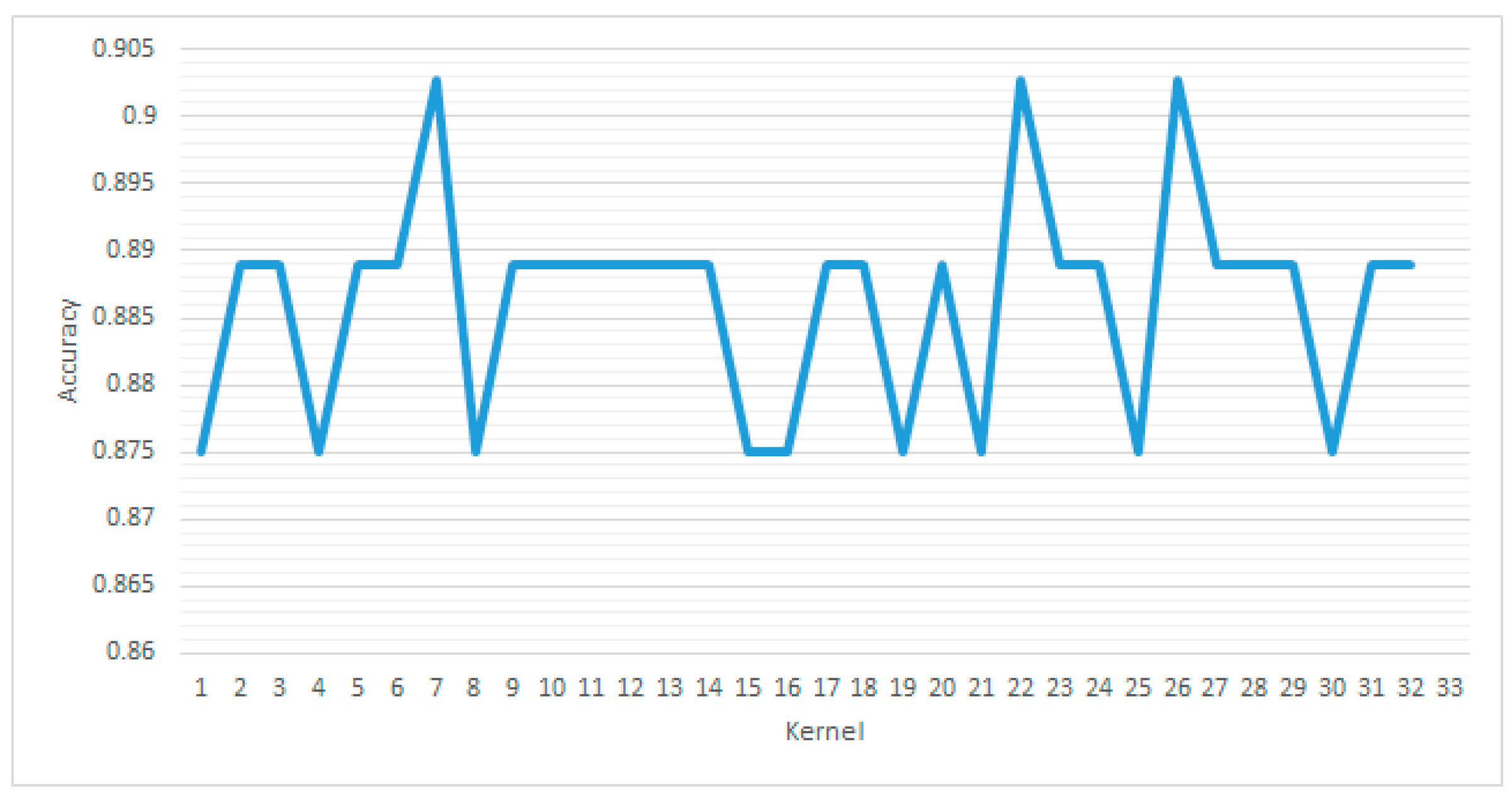
In this study, we used the MNE Sample Dataset [13] as the source of input EEG signals. The EEGNet architecture was configured with F1 = 32 temporal filters and a depth multiplier D = 8, and trained to establish a baseline performance. The resulting baseline accuracy was 0.889. To investigate the robustness of individual filters, we subsequently injected noise into each of the 32 Conv2D kernels (temporal filters) one at a time. Specifically, we replaced the weights of each kernel with 3 dB white noise and evaluated the resulting inference performance. This procedure enables the assessment of the impact of noise on model accuracy at a per-filter level. Figure 3 presents the experimental results, showing how each kernel contributes to the model’s robustness and performance degradation under noisy conditions.

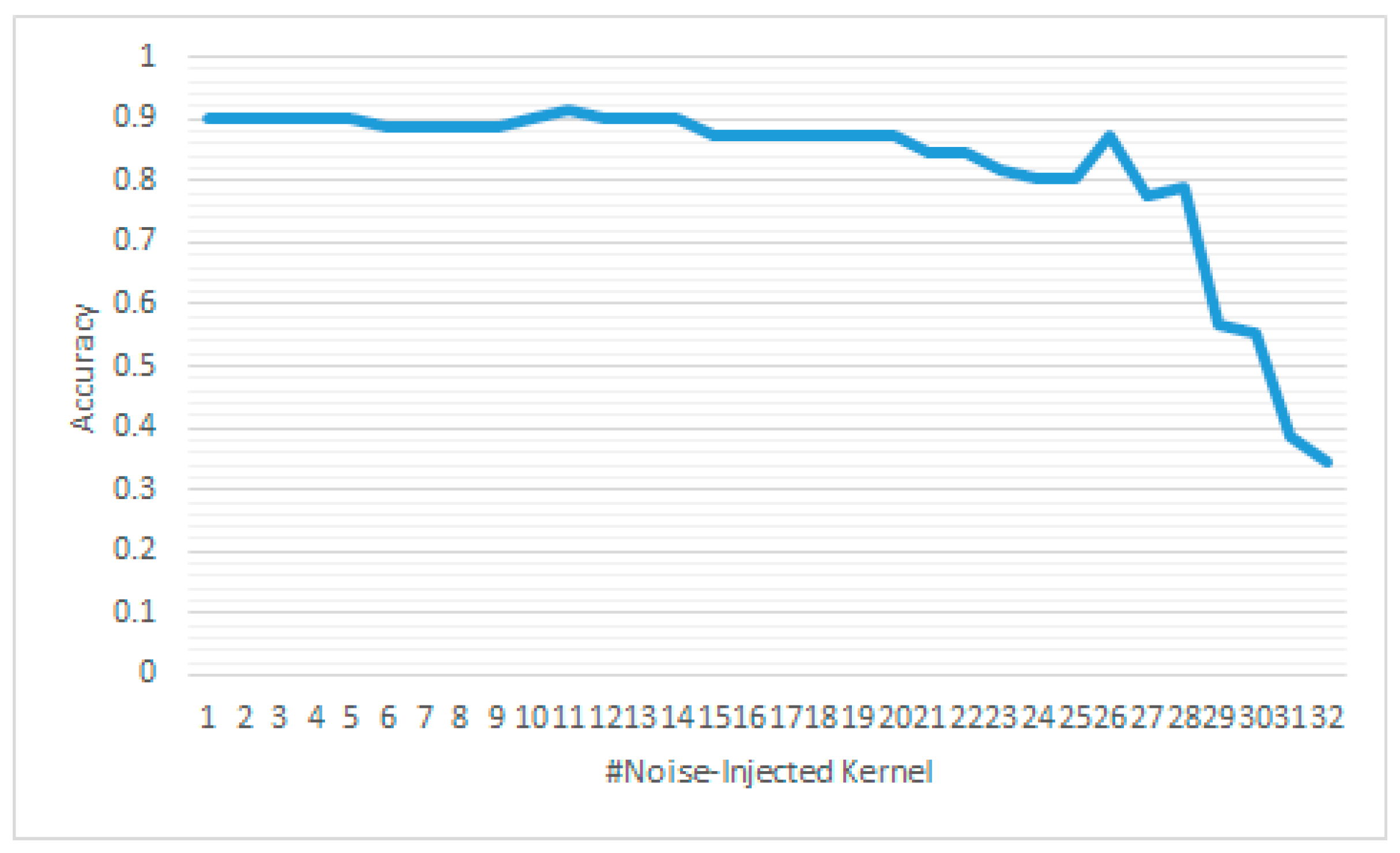
After obtaining the inference results for individual kernel noise injection, we ranked all Conv2D kernels based on the corresponding classification accuracy, with the highest accuracy placed at the top of the list. Then, we gradually increased the number of kernels subjected to noise injection, following this ranked order, and recorded the resulting inference accuracy at each step. Figure 4 presents the experimental results, where the x-axis represents the number of Conv2D kernels injected with noise, and the y-axis indicates the corresponding inference accuracy.

When noise is injected into the 15th Conv2D kernel, the inference accuracy drops from 0.903 (which is higher than the baseline accuracy) to 0.875. This suggests that removing 14 of the 32 Conv2D kernels preserves comparable inference performance. Based on this observation, we modified the EEGNet model by reducing the number of temporal filters to F1 = 18 (with D = 8) and retrained the model. The simplified model achieved an inference accuracy of 0.875, which is consistent with our expectation.

5. Conclusions

We investigated the effect of injecting noise into individual Conv2D kernels in the EEGNet architecture. By ranking kernels based on their sensitivity to noise, we identified a subset of filters that have minimal impact on inference accuracy. The results demonstrate that it is possible to reduce the number of temporal filters from 32 to 18 while maintaining comparable classification performance. The simplified model not only reduces computational complexity but also maintains an inference accuracy of 0.875, closely matching that of the original full model. These findings suggest a practical strategy for kernel-level pruning and model compression in EEG-based deep learning applications. While the current results demonstrate that kernel-level noise injection can be used as an effective strategy for identifying redundant filters and simplifying EEGNet, future exploration is still required.

First, the method developed can be extended to other layers of the network, such as depthwise or separable convolutions, to evaluate the broader impact of noise on spatial and temporal feature representations. Second, more advanced noise-based pruning strategies, such as adaptive thresholding or gradient-guided perturbations, need to be tested for enhanced model compression without compromising performance. Additionally, it is necessary to validate the developed method across multiple EEG datasets and BCI paradigms to assess its generalizability. Finally, implementing this technique in real-time or on embedded hardware platforms may lead to practical applications in mobile or wearable BCI systems with strict computational constraints.