Sensor Fusion of Doppler Microwave and Multizone ToF for Short-Range Dynamic Object Tracking ^†

Abstract

We present a low-cost sensor-fusion system combining a 10.525 GHz CW Doppler microwave sensor with an 8 × 8 Time-of-Flight (ToF) infrared sensor for short-range object tracking. Data are acquired and processed in a sequential fusion pipeline: ToF-based Convolutional Neural Networks (CNNs) estimate object presence, coordinates, and cross-section, while Doppler histograms yield radial velocity; outputs are then fused at the decision level. A dataset of 31,367 frames was collected. The system tracks objects (≥35 cm²) at speeds up to 10 m/s within 5–250 cm, achieving 98% detection and 84% positioning accuracy. This approach offers radar-like capabilities at a reduced cost, enabling applications in industrial, and consumer-electronics domains.

1. Introduction

Tracking and positioning fast-moving objects in a short range is of particular importance in industrial applications. With the growing demands of manufacturing, robotics, and security systems, there has been increasing interest in short-range systems capable of detecting and characterizing fast-moving objects [1]. In robotics, in particular, rising production volumes and the resulting price pressure have driven the need for lower-cost sensing solutions [2].

However, ultra-low-cost single sensors struggle to meet these requirements on their own. Continuous-wave (CW) microwave Doppler sensors can reliably provide radial velocity information, yet they cannot offer spatial positioning of the object [3,4,5]. Multi-zone Time-of-Flight (ToF) sensors, on the other hand, enable spatial analysis but are limited by low frame rates, very low resolution, and susceptibility to environmental conditions, making them insufficient as a standalone solution [6,7,8].

In this study, we developed a low-cost, easily integrable sensor system capable of determining not only the three-dimensional coordinates of the tracked object but also its radial velocity and cross-sectional area. By interpreting and fusing the outputs of two different sensor types using artificial intelligence models, our system can fulfill requirements typically met only by far more expensive radar sensor systems [9,10].

1.1. Microwave Doppler Sensing

Microwave Doppler sensors are a type of device that detect the velocity of target objects by utilizing the Doppler principle [3,4]. These sensors are equipped with both transmitting and receiving antennas that operate at high frequencies. In the type used in our study, the continuous wave transmitter typically operates at frequencies around 10 GHz. On the receiving side, the reflected signal is mixed in an oscillator to obtain the in-phase (I) and quadrature (Q) components [11,12]. This enables the capture of both amplitude-time envelopes and phase information, allowing the instantaneous phase difference to be used to determine the sign of the velocity through arctangent demodulation. The Doppler frequency shift can be calculated as shown in Equation (1) [13].

$$f_d={\displaystyle \frac{2\nu }{\lambda }}\cos \left(\theta \right); \lambda \approx 2.85 \mathrm{cm}$$

(1)

Based on the applied formula, an object with a radial velocity of 1 m/s produces a Doppler frequency shift of approximately 70 Hz [13]. However, CW Doppler systems are sensitive only to radial velocities; during purely lateral movements (θ = 90°), no frequency shift is observed. Moreover, they provide no information about the absolute range or physical properties of the target. Reflections caused by vibrations can introduce noise, and frequency shifts from other moving objects in the environment may also be detected. Therefore, strong filtering techniques should be applied in practical implementations, and the transmitter beam should be mechanically directed toward the target object to improve measurement reliability [14,15].

1.2. Multizone Time-of-Flight Sensors

Infrared (IR) Time-of-Flight sensors are specialized distance measurement devices equipped with an emitter IR LED and a corresponding receiver photodiode [16]. They operate by calculating the time it takes for IR light emitted from the LED to reflect off a target object and return to the photodiode. In addition to one-dimensional measurements, modern sensors can integrate multiple emitter LEDs placed at different angles, enabling two-dimensional distance measurements. Sensors capable of operating in 3 × 3, 4 × 4, and 8 × 8 matrix configurations can measure in the IR band with integrated electronics sensitive enough to calculate delays at the speed of light, while still being accessible for low-cost applications [17,18].

Multi-zone ToF sensors can provide object distance measurements with sub-centimeter precision and, despite their low resolution, can also contribute to determining the spatial coordinates of objects [18]. However, these sensors generally suffer from both low spatial resolution and low frame rates. Compared to radar systems, the significantly lower frame rate makes it difficult to track fast-moving objects, and calculating velocity is not possible for objects that pass through the field of view faster than a few acquisition windows. Therefore, these sensors are typically used for detecting or locating stationary or slow-moving objects [19,20].

In this study, ToF sensors and CW Doppler microwave sensors were positioned on the same plane to enable synchronized data acquisition. This arrangement allowed the high-accuracy position information from the ToF sensor to be complemented by the high temporal resolution and velocity measurement capability of the Doppler sensor [21,22]. The strengths of both sensors were integrated into a single fusion model via a machine learning pipeline.

This work presents an artificial intelligence-based fusion architecture that adaptively combines CW Doppler and 8 × 8 ToF sensors for low-cost, short-range applications. The main innovations can be summarized as: (1) synchronized hardware setup, (2) a unified CNN+MLP-based estimation model, and (3) a multi-class dataset containing 70,000 labeled entries.

2. Materials and Methods

In this study, a 10.525 GHz CW Doppler microwave sensor and an 8 × 8 ToF sensor (STMicroelectronics, Geneva, Switzerland) were placed on the same plane. An analog signal conditioning circuit was employed to digitize the Doppler sensor output, and a microwave shielding cage was constructed around the sensor to reduce unwanted microwave transmission. The ToF sensor was positioned next to the microwave sensor cage to ensure operation within the same field of view [4].

Sensor data was collected using an STM32F407 (STMicroelectronics, Geneva, Switzerland) microcontroller, where software-based filters were applied. The processed data was then transferred to a computer via a serial port. Manual labeling was performed using a custom graphical user interface (GUI) developed in Python 3.10.12. A total of 411 distinct object measurements resulted in the creation of 31,367 ToF measurement matrices and 8220 Doppler frequency histograms [23].

Using the recorded dataset, a multi-layer machine learning pipeline was developed. The pipeline first checks for the presence of an object. If an object is detected, it subsequently predicts the spatial coordinates (X, Y, and depth), the instantaneous radial velocity relative to the sensor, and the object’s cross-sectional area. These outputs enabled the positioning and tracking of objects at distances up to 250 cm and speeds up to 10 m/s.

2.1. Microwave Doppler

In our research, we used an HB100-type CW Doppler sensor module capable of providing a frequency output. Operating at 10.525 GHz, the sensor consists of a Dielectric Resonator Oscillator (DRO), a microwave mixer, and a patch antenna. It directly outputs the Doppler frequency shift through its Intermediate Frequency (IF) pin [4,9].

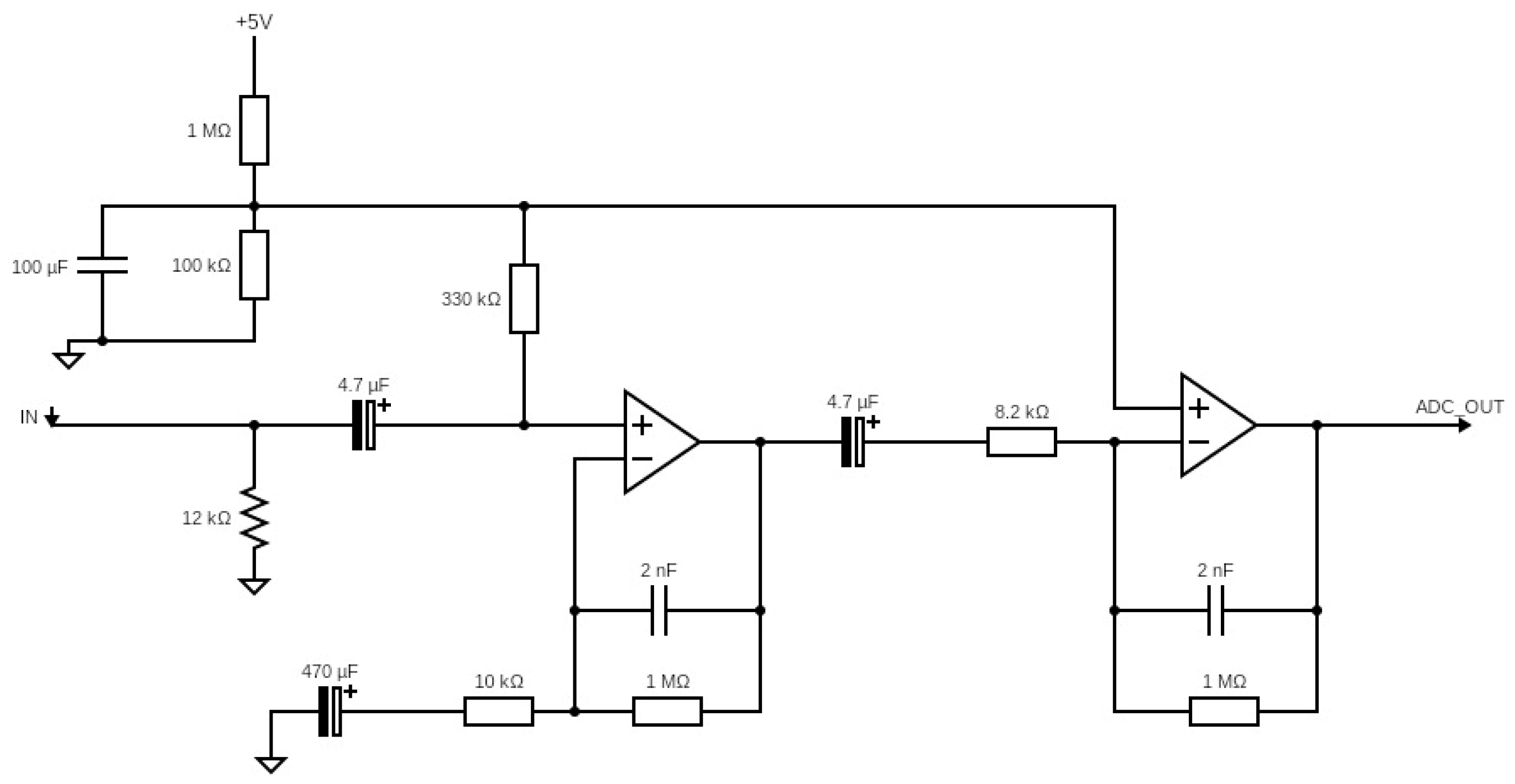
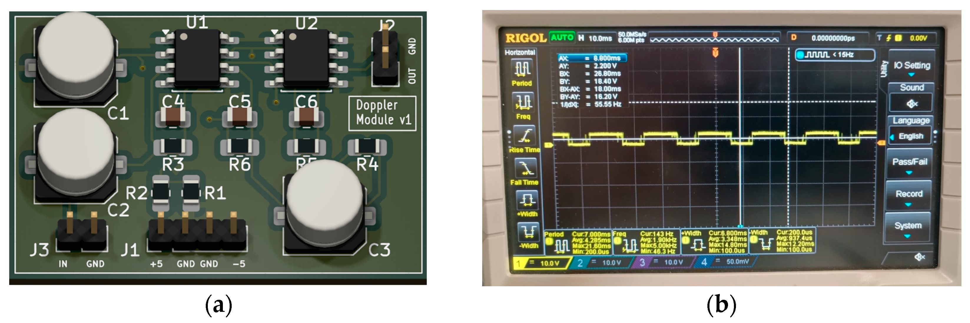
To digitize the signal coming from the IF pin of the microwave sensor, it must first be amplified, rectified, and converted into a square wave. For this purpose, an analog signal conditioning circuit whose schematic is shown in Figure 1. Printed board circuit (PCB) design shown in Figure 2a. Figure 2b shows the square-wave output of this analog circuit. Since the frequency of the resulting square wave is directly equal to the Doppler frequency, the velocity of objects can be calculated by applying the frequency–velocity relationship [3].

The output from the microwave signal processing circuit is captured and digitized by the microcontroller. At this stage, a 1.2 kHz digital low-pass filter is applied. As shown in Equation (2), 1.2 kHz corresponds to a velocity of 17.1 m/s, which is above the research target of 10 m/s; therefore, filtering was implemented [3].

$$f_{d,max}={\displaystyle \frac{2{\nu }_{max}}{2.85 \mathrm{c}\mathrm{m}}}\times 1\to {\nu }_{max}\approx 17.1 \mathrm{m}/\mathrm{s}$$

(2)

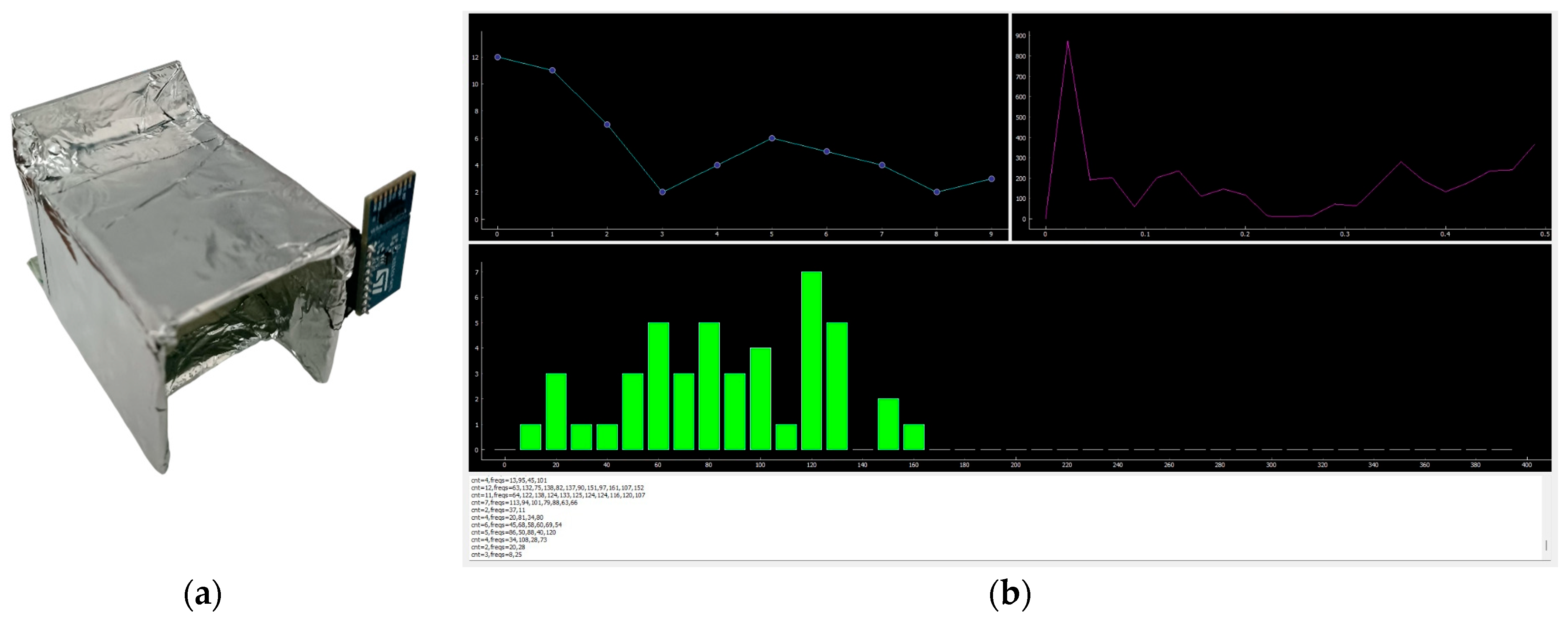
Additionally, the microwave sensor emits in all directions, which may result in noise from movements or vibrations of non-target objects being recorded. To limit detection to the target direction only, five sides of the sensor were covered with FR4 copper plates and thin aluminum foil, creating a directional microwave enclosure. The constructed microwave cage is shown in Figure 3.

2.2. Multizone ToF Sensor

In this study, the VL53L5CX-SATEL (STMicroelectronics, Geneva, Switzerland) sensor module was used for distance measurement and spatial position determination. The sensor’s control and data acquisition were carried out via an STM microcontroller, allowing the ToF data to be read directly from the microcontroller and synchronized to the same time axis as the Doppler sensor. Figure 3a shows the ToF sensor positioned next to the Doppler sensor.

The system was operated in an 8 × 8 matrix mode, collecting data from a total of 64 independent zones. For each pixel, the following information was obtained: ambient light intensity (Kcps/spads), target presence estimated by the sensor’s internal histogram-based algorithm, target distance (in mm), and target pixel status. In this mode, the sensor recorded measurements at 10 Hz. The collected multidimensional ToF data were structured to include the 8 × 8 distance matrix for each frame, along with pixel-based target status and ambient light information.

The microcontroller transmitted the raw 64-zone ToF data to a computer, where a Python-based interface application was used for manual labeling with corresponding X, Y, and cross-section information. In total, 256 features were stored for each measurement.

2.3. Dataset Preperation

In line with the study objectives, measurements of objects from multiple classes, at different speeds and positions, were conducted using two different sensors. For the ToF sensor, spatial coordinates and cross-section information were labeled. Using four different objects with varying cross-sections, the X and Y coordinates were determined either manually through labeling or by positioning according to the data. A total of 31,367 unique data entries were collected, of which 25,092 were labeled as containing objects, and ~6000 were labeled as empty class. Care was taken to ensure a balanced distribution of different object classes and coordinate values during dataset creation.

For cross-section data, four different experimental balls with diameters of 7, 10, 15, and 17 cm were selected. The actual cross-section areas correspond to approximately 38 cm², 78 cm², 132 cm², and 176 cm², respectively. These values were classified numerically from 1 to 4 in the cross-section dataset.

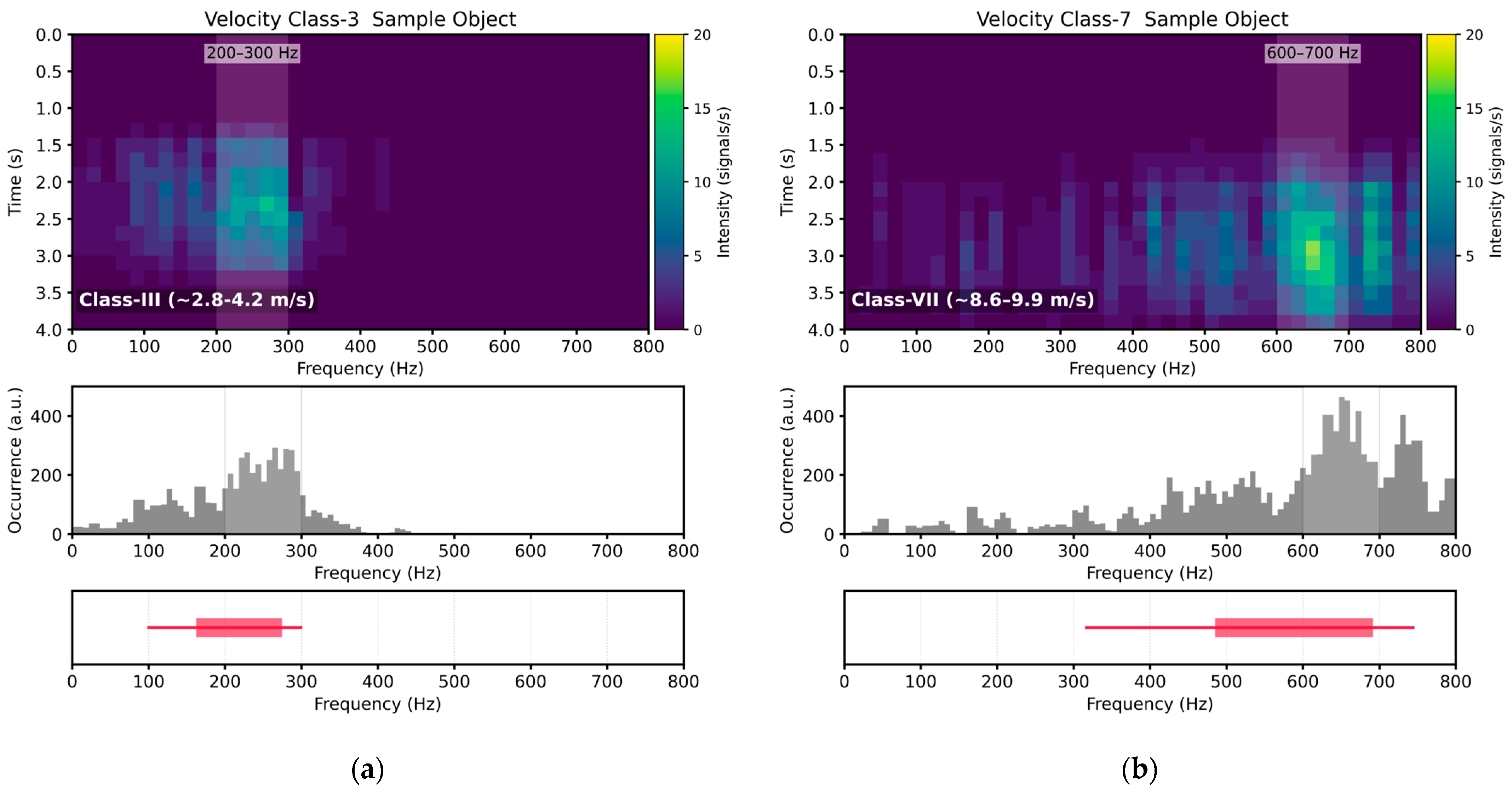
For the microwave sensor, one of eight different velocity classes was manually selected for each test. Since the sensor cannot clearly measure objects moving with acceleration directly in front of it, the sensor data were approximately labeled and classified according to the ranges shown in

Table 1. Doppler Microwave Class Ranges.

Class	Doppler Freq. Range (Hz)	Velocity (m/s)
Velocity Class-1	~0–100 Hz	~0.0–1.4 m/s
Velocity Class-2	~100–200 Hz	~1.4–2.8 m/s
Velocity Class-3	~200–300 Hz	~2.8–4.2 m/s
Velocity Class-4	~300–400 Hz	~4.2–5.7 m/s
Velocity Class-5	~400–500 Hz	~5.7–7.1 m/s
Velocity Class-6	~500–600 Hz	~7.1–8.6 m/s
Velocity Class-7	~600–700 Hz	~8.6–9.9 m/s
Velocity Class-8	~700–800 Hz	~9.9+ m/s

.

Figure 4 presents Doppler measurement results in the frequency–time domain for three different velocity classes, illustrating the shift of the dominant frequency point in the histogram as velocity increases.

In total, 8220 Doppler frequency histograms were obtained from moving objects. Since 411 distinct object passages were recorded, the complete dataset was divided to produce 411 images. Each image was generated at a resolution of 40 × 20 pixels, representing the time–frequency histogram plane, and constructed from histograms of frequencies within the 0–800 Hz band.

2.4. Model Development

The developed model is a three-stage supervised learning pipeline. In the first stage, the model performs binary classification to determine the presence or absence of an object. If an object is detected, spatial coordinates (X,Y), and the class of its cross-sectional area is determined. All training and testing procedures were implemented in Python.

Object detection, coordinate prediction, and cross-section prediction modules were trained independently. A total of 31,367 data samples were used. Of these, 25,092 samples were allocated for model development, with an 80–20% split between training and testing subsets. The remaining data samples were used to simultaneously evaluate the performance of all three trained models in a single testing procedure.

2.4.1. Object Detection Architecture

For object detection, we used the matrix data obtained from the ToF sensor. We employed a customized convolutional neural network (CNN) model, which begins with two convolutional layers, each using a 3 × 3 kernel followed by a ReLU activation function. The first convolutional layer maps the single input channel to 16 feature maps, and the second maps these 16 features into 32 features. The resulting feature maps are flattened and passed through a fully connected layer with 32 × H × W units and 128 output features, followed by a ReLU activation. Finally, the resulting layer maps 128 features into a single output neuron as a raw logit value. A threshold value of 0.5 was applied to determine the binary classification output. The model was trained with a learning rate of 1 × 10⁻³ for 50 epochs [24].

2.4.2. Cross-Section Prediction Architecture

The cross-section classification module employed the same CNN architecture used for object detection, with the output layer adapted to predict discrete cross-section classes ranging from 1 to 4. The model was trained using a learning rate of 1 × 10⁻³ for 80 epochs.

2.4.3. Coordinate Prediction Architecture

The coordinate prediction module used the same CNN architecture as the object detection model, except the final fully connected layer mapped 128 features into two output neurons, corresponding to the X and Y coordinates in ToF matrix. Both coordinates could take integer values from 1 to 8, representing positions within the 8 × 8 ToF grid. The model was trained with a learning rate of 1 × 10⁻³ for 70 epochs to enable accurate spatial localization.

2.4.4. Radial Velocity Prediction Architecture

The radial velocity prediction stage uses frequency–intensity versus time heatmaps, generated from the histograms of the Doppler microwave sensor, at a resolution of 40 × 20 pixels. To estimate speed from these heatmap images, a pretrained ResNet18 model was employed. The network was fine-tuned using a dataset of 411 images, split into 80% for training and 20% for testing. Training was performed with a learning rate of 1 × 10⁻⁴ over 20 epochs.

2.4.5. Model Fusion

The model fusion pipeline operates sequentially, with each stage building on the outputs of the previous one. The process begins with the object detection model; if an object is detected, the coordinate prediction and cross-section classification modules are executed.

Finally, the radial velocity estimation stage is performed using Doppler microwave sensor data. Through this layered approach, all necessary parameters of the tracked target are obtained. Since both spatial location and velocity are available, additional orientation tracking can be implemented through software algorithms [25].

3. Results

In the results, Doppler microwave sensor data were processed by selecting the 0–800 Hz frequency range and constructing histograms to represent the distribution of Doppler shifts over time, can be seen on Figure 4. Similarly, the multizone ToF sensor produced 8 × 8 depth matrices for each frame, capturing spatial distance information across 64 zones.

3.1. Model Results

The developed multi-stage supervised learning framework was evaluated across all sub-modules, both individually and in the integrated fusion pipeline.

3.1.1. Object Detection

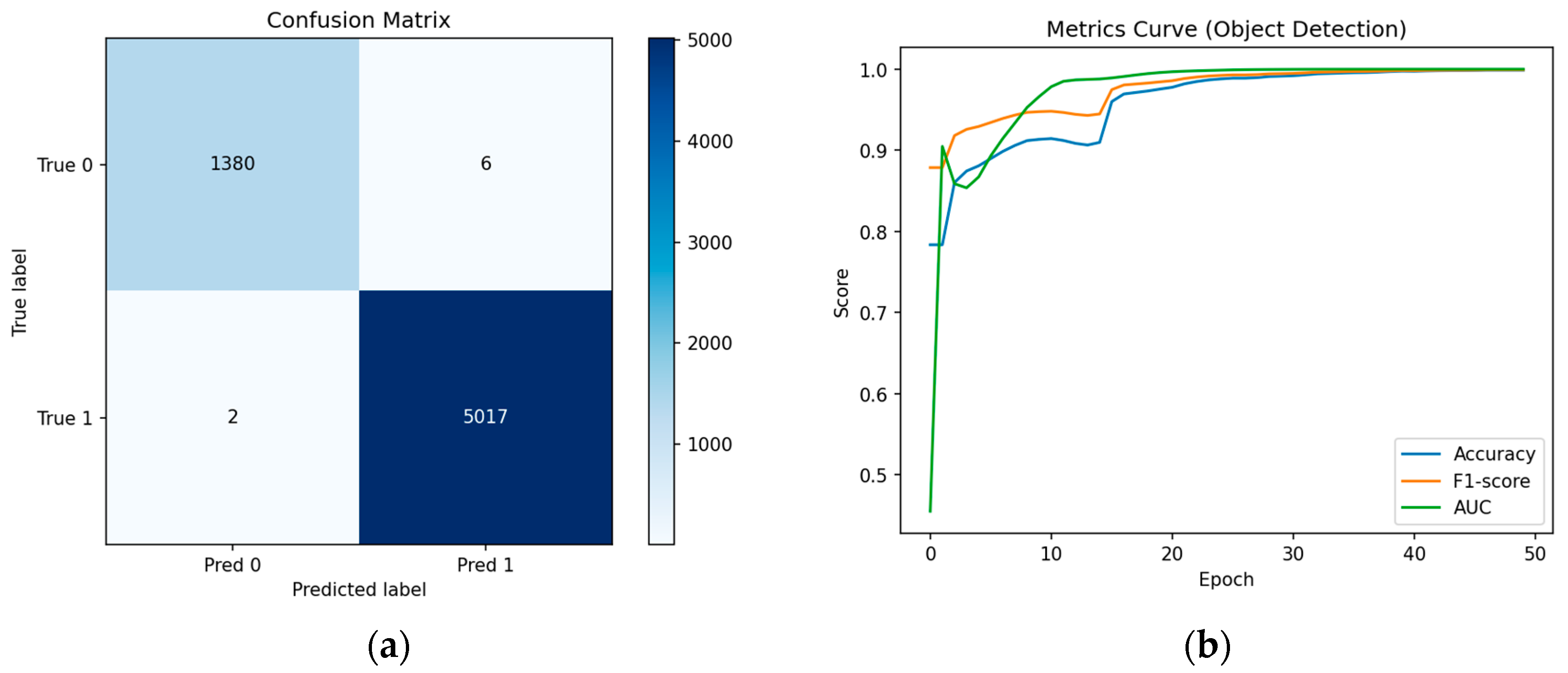
The customized CNN-based object detection module achieved near perfect results on the test set, with a validation loss of 0.0093, an accuracy of 99.88%, and an F1-score of 0.9992. The mean absolute error (MAE) was 0.0012, and the root mean squared error (RMSE) was 0.0353, indicating near-perfect binary classification performance for object presence. The confusion matrix for classification is shown in Figure 5a, while the training metrics versus epoch results are presented in Figure 5b.

3.1.2. Cross-Section Prediction

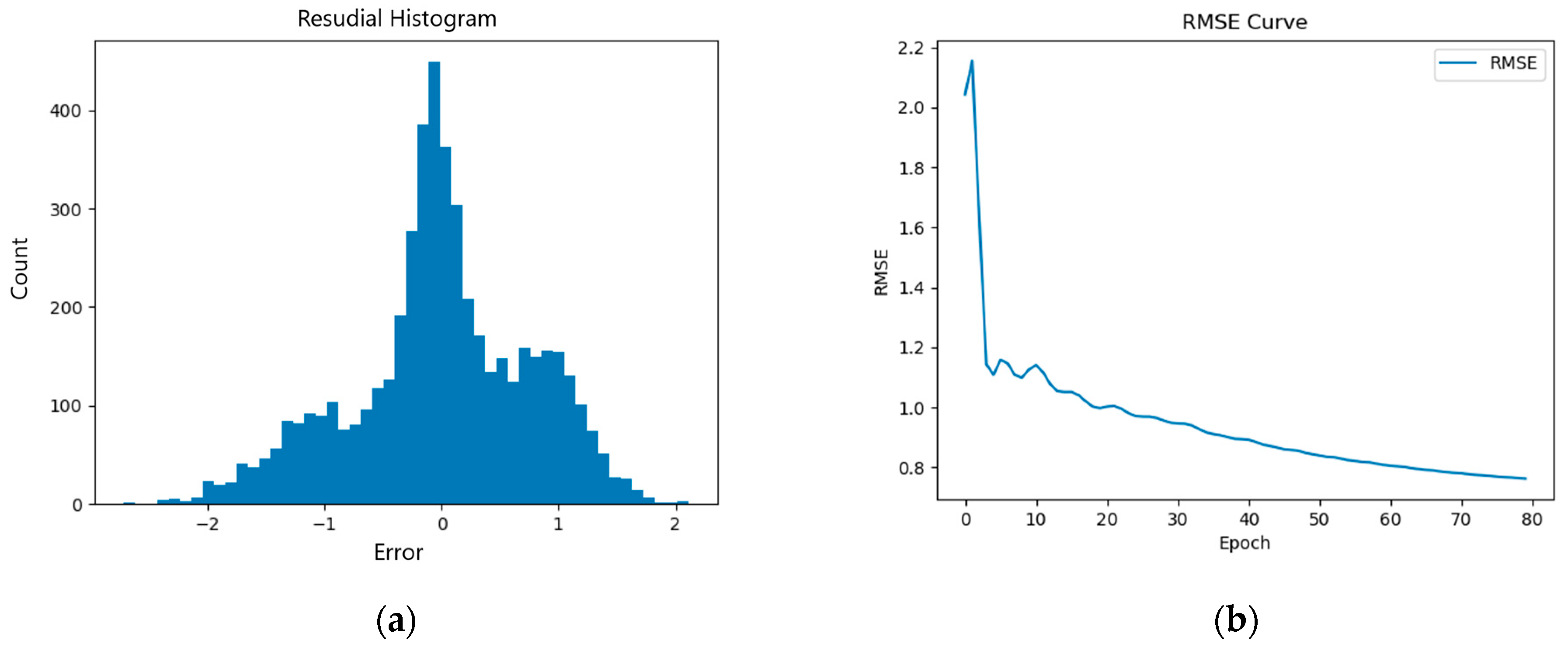
The cross-section classification module employed reached a validation loss of 0.5814, RMSE of 0.7625, and MAE of 0.5833. The coefficient of determination (R²) was 0.4940, showing moderate correlation between predictions and ground truth in this regression-style classification task. Figure 6a, while the RMSE versus epoch plot during training is presented in Figure 6b.

3.1.3. Coordinate Prediction

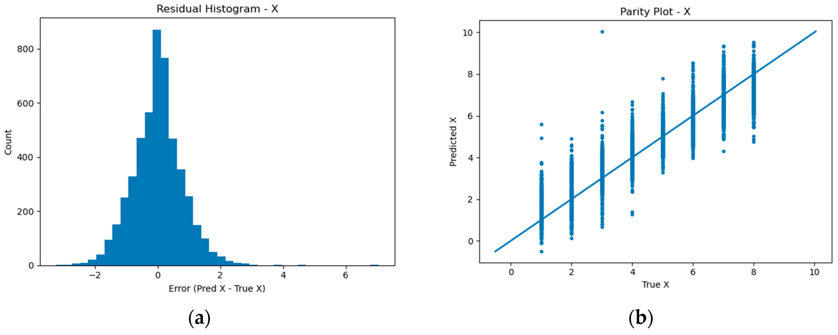
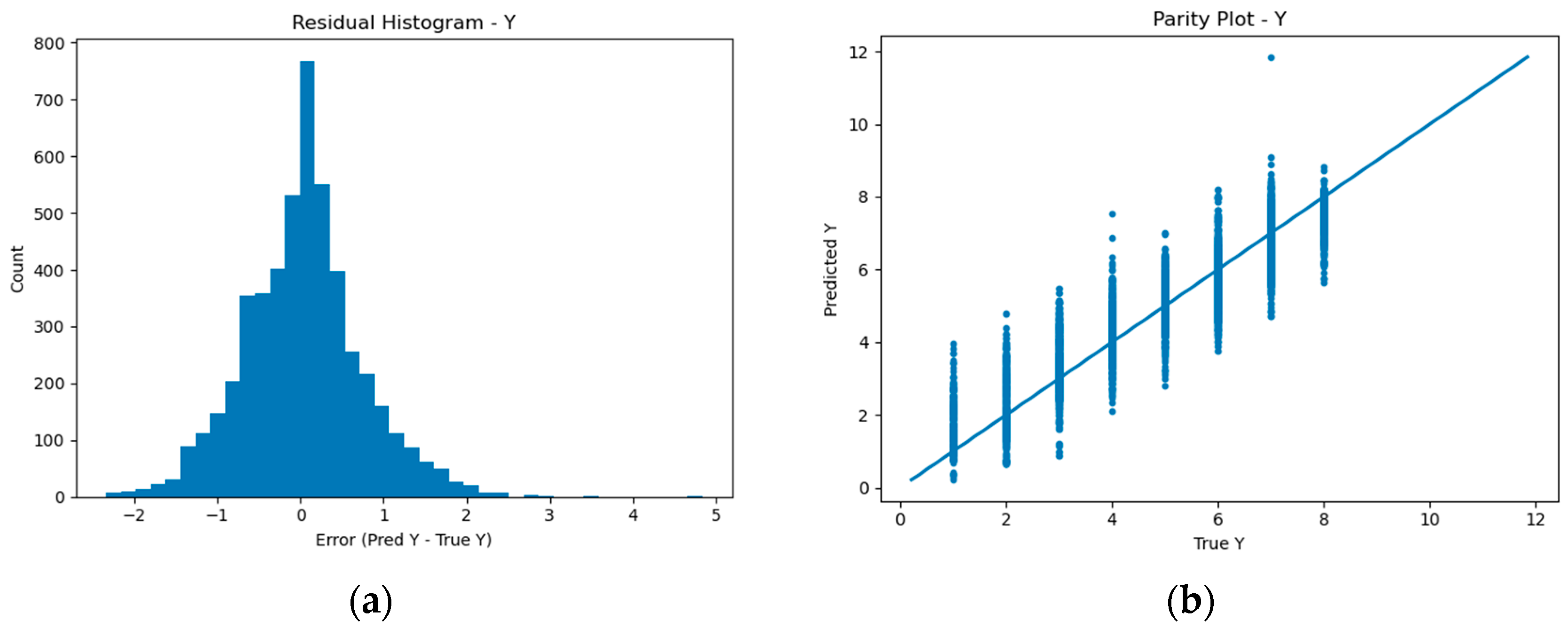
The results of the prediction model are shown for the X-axis in Figure 7a,b, and for the Y-axis in Figure 8a,b.

3.1.4. Radial Velocity Prediction

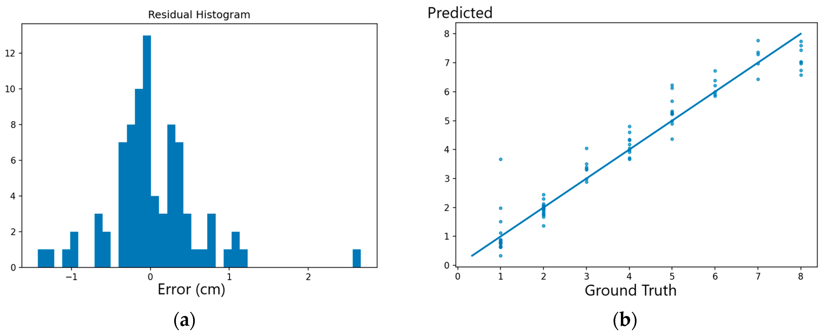
The radial velocity prediction results showed that the model performed best in the lower speed range, with higher accuracy and lower error values. In the lower velocity range (class 1 to 5), it achieved an MAE of 0.3422 and RMSE of 0.5287, corresponding to 79.69% accuracy within 93.75% within ±1 unit. Performance decreased in the higher (class 6 to 8) range, where the MAE rose to 0.5505 and RMSE to 0.6873, with accuracies of and 84.21% (±1). Details can be found in Figure 9a,b.

Overall, for all 83 test samples, the model recorded an MAE of 0.3899, RMSE of 0.5690, 91.57% accuracy at ±1 unit of the ground truth value. Results can be seen in

Table 2. Performance results of radial velocity prediction.

Class Range	Velocity Range	MAE	RMSE	Acc@ ± 1
Class 1 to 5	0.0–7.1 m/s	0.34	0.53	93.7%
Class 6 to 8	+7.1 m/s	0.55	0.69	84.2%

.

3.1.5. Model Evolution

In the final integrated testing procedure, the object detection model was executed first; upon detecting an object, the coordinate prediction and cross-section estimation modules were run sequentially.

The combined results were as follows:

• Object detection MAE = 0.0027 with an accuracy of 99.67%
• X coordinate prediction MAE = 0.6255 with ±1 unit accuracy of 77.93%,
• Y coordinate prediction MAE = 0.5626 with ±1 unit accuracy of 81.94%
• Cross MAE = 0.7598 with ±1.41 unit accuracy of 84.06%.
• Radial velocity prediction gives 91.57% accuracy at ±1 unit of the ground truth value.

The slightly higher MAE values compared to individual model evaluations are likely due to distributional differences between the datasets used for standalone training/testing and the final combined evaluation. The ±1 unit accuracy threshold for X and Y coordinates reflects the smallest measurable positional change in the hardware, while the ±1.4 unit threshold for cross-section size corresponds to the Euclidean displacement of 1 unit in both X and Y directions.

4. Discussion

In this study, we demonstrated a low-cost method that fuses ToF and Doppler sensors to obtain both the radial velocity and spatial position of a target. By combining the high spatial accuracy of the ToF sensor with the high temporal resolution of the Doppler sensor, the proposed system provides an effective solution for short-range, high-speed object tracking. The modular architecture allowed each component to be independently optimized, resulting in high accuracy for both position and velocity estimation.

The results indicate that low-cost sensors, when paired with effective data fusion techniques, can deliver high performance in fields such as industrial automation, robotics, and security. However, performance may be affected by varying environmental conditions, target sizes, and velocity ranges. Future work could focus on increasing sensor resolution, training models on larger and more diverse datasets, and integrating the system into real-time applications to expand its practical usability.

References

1. Kalsoom, T.; Ramzan, N.; Ahmed, S.; Ur-Rehman, M. Advances in Sensor Technologies in the Era of Smart Factory and Industry 4.0. Sensors 2020, 20, 6783. [Google Scholar] [CrossRef] [Scilit] [PubMed]
2. Folgado, F.J.; Calderón, D.; González, I.; Calderón, A.J. Review of Industry 4.0 from the Perspective of Automation and Supervision Systems: Definitions, Architectures and Recent Trends. Electronics 2024, 13, 782. [Google Scholar] [CrossRef] [Scilit]
3. Mandal, P.; Roy, L.P.; Das, S.K. Flying Objects Classification Based on Micro–Doppler Signature Data from UAV Borne Radar. IEEE Geosci. Remote Sens. Lett. 2024, 21, 3501605. [Google Scholar] [CrossRef] [Scilit]
4. Thiel, D.V.; Cabrita, J.; Fickenscher, T.; Espinosa, H.G. Low-Cost X-Band Doppler Radar for Nadir Velocity Detection. In Proceedings of the 2025 6th Australian Microwave Symposium (AMS), Gold Coast, Australia, 10–11 February 2025; pp. 1–2. [Google Scholar] [CrossRef] [Scilit]
5. Soumya, A.; Krishna Mohan, C.; Cenkeramaddi, L.R. Recent Advances in MmWave-Radar-Based Sensing, Its Applications, and Machine Learning Techniques: A Review. Sensors 2023, 23, 8901. [Google Scholar] [CrossRef] [Scilit]
6. Senel, N.; Kefferpütz, K.; Doycheva, K.; Elger, G. Multi-Sensor Data Fusion for Real-Time Multi-Object Tracking. Processes 2023, 11, 501. [Google Scholar] [CrossRef] [Scilit]
7. Khaleghi, B.; Khamis, A.; Karray, F.O.; Razavi, S.N. Multisensor Data Fusion: A Review of the State-of-The-Art. Inf. Fusion 2013, 14, 28–44. [Google Scholar] [CrossRef] [Scilit]
8. Kim, D.K.; Kim, Y. Quadrature Frequency-Group Radar and Its Center Estimation Algorithms for Small Vibrational Displacement. Sci. Rep. 2019, 9, 6763. [Google Scholar] [CrossRef] [Scilit]
9. Kong, H.; Huang, C.; Yu, J.; Shen, X. A Survey of MmWave Radar-Based Sensing in Autonomous Vehicles, Smart Homes and Industry. IEEE Commun. Surv. Tutor. 2024, 27, 463–508. [Google Scholar] [CrossRef] [Scilit]
10. Lv, W.; He, W.; Lin, X.; Miao, J. Non-Contact Monitoring of Human Vital Signs Using FMCW Millimeter Wave Radar in the 120 GHz Band. Sensors 2021, 21, 2732. [Google Scholar] [CrossRef] [Scilit]
11. Pour Ebrahim, M.; Sarvi, M.; Yuce, M. A Doppler Radar System for Sensing Physiological Parameters in Walking and Standing Positions. Sensors 2017, 17, 485. [Google Scholar] [CrossRef] [Scilit]
12. Li, C.; Lubecke, V.M.; Boric-Lubecke, O.; Lin, J. A Review on Recent Advances in Doppler Radar Sensors for Noncontact Healthcare Monitoring. IEEE Trans. Microw. Theory Tech. 2013, 61, 2046–2060. [Google Scholar] [CrossRef] [Scilit]
13. Islam, S.M.M.; Fioranelli, F.; Lubecke, V.M. Can Radar Remote Life Sensing Technology Help Combat COVID-19? Front. Commun. Netw. 2021, 2, 648181. [Google Scholar] [CrossRef] [Scilit]
14. Kim, H.; Jeong, J. Non-Contact Measurement of Human Respiration and Heartbeat Using W-Band Doppler Radar Sensor. Sensors 2020, 20, 5209. [Google Scholar] [CrossRef] [Scilit] [PubMed]
15. Wang, Y.; Wang, W.; Zhou, M.; Ren, A.; Tian, Z. Remote Monitoring of Human Vital Signs Based on 77-GHz Mm-Wave FMCW Radar. Sensors 2020, 20, 2999. [Google Scholar] [CrossRef] [Scilit]
16. Kolb, A.; Barth, E.; Koch, R.; Larsen, R. Time-of-Flight Cameras in Computer Graphics. Comput. Graph. Forum 2010, 29, 141–159. [Google Scholar] [CrossRef] [Scilit]
17. Gokturk, S.B.; Yalcin, H.; Bamji, C. A Time-Of-Flight Depth Sensor-System Description, Issues and Solutions. Available online: https://ieeexplore.ieee.org/abstract/document/1384826 (accessed on 19 July 2021).
18. Foix, S.; Alenya, G.; Torras, C. Lock-in Time-of-Flight (ToF) Cameras: A Survey. IEEE Sens. J. 2011, 11, 1917–1926. [Google Scholar] [CrossRef] [Scilit]
19. He, Y.; Liang, B.; Zou, Y.; He, J.; Yang, J. Depth Errors Analysis and Correction for Time-of-Flight (ToF) Cameras. Sensors 2017, 17, 92. [Google Scholar] [CrossRef] [Scilit] [PubMed]
20. Zoghlami, F.; Sen, O.K.; Heinrich, H.; Schneider, G.; Ercelik, E.; Knoll, A.; Villmann, T. ToF/Radar Early Feature-Based Fusion System for Human Detection and Tracking. In Proceedings of the 2021 22nd IEEE International Conference on Industrial Technology (ICIT), Valencia, Spain, 10–12 March 2021. [Google Scholar] [CrossRef] [Scilit]
21. Kaul, C.; Mitchell, K.J.; Kassem, K.; Tragakis, A.; Kapitany, V.; Starshynov, I.; Villa, F.; Murray-Smith, R.; Faccio, D. AI-Enabled Sensor Fusion of Time-of-Flight Imaging and MmWave for Concealed Metal Detection. Sensors 2024, 24, 5865. [Google Scholar] [CrossRef] [Scilit]
22. Qi, C.; Song, C.; Zhang, N.; Song, S.; Wang, X.; Xiao, F. Millimeter-Wave Radar and Vision Fusion Target Detection Algorithm Based on an Extended Network. Machines 2022, 10, 675. [Google Scholar] [CrossRef] [Scilit]
23. McGuire, K.; de Croon, G.; De Wagter, C.; Tuyls, K.; Kappen, H. Efficient Optical Flow and Stereo Vision for Velocity Estimation and Obstacle Avoidance on an Autonomous Pocket Drone. IEEE Robot. Autom. Lett. 2017, 2, 1070–1076. [Google Scholar] [CrossRef] [Scilit]
24. O’Shea, K.; Nash, R. An Introduction to Convolutional Neural Networks. arXiv 2015, arXiv:1511.08458. [Google Scholar] [CrossRef] [Scilit]
25. He, K.; Zhang, X.; Ren, S.; Sun, J. Deep Residual Learning for Image Recognition. arXiv 2015, arXiv:1512.03385. [Google Scholar] [CrossRef] [Scilit]
Figure 1. Schematic of Microwave Doppler signal conditioner circuit.
Engproc 118 00099 g001
Figure 2. Microwave signal conditioning circuit: (a) Printed circuit board of the circuit, (b) oscilloscope screen capture of the square-wave output from the circuit with the HB100 and our prototype circuit module connected.
Engproc 118 00099 g002
Figure 3. Doppler microwave: (a) External view of the copper plate–aluminum cage, (b) circuit outputs displayed in the Python interface used for recording real time microwave Doppler sensor data: top left: frequency intensity over the last 10 s, top right: FFT results, and bottom: histogram view.
Engproc 118 00099 g003
Figure 4. In the top plot, the microwave frequency histogram–time plots show frequency increasing toward the right, with higher values indicating stronger intensity. The middle plot displays the frequency histogram. In the bottom candlestick chart, dominant frequencies are shown as thick red candles, while weaker repeating frequencies are represented as thin red candles. (a) presents the heatmap of a low-speed object, and (b) shows the heatmap of a high-speed object.
Engproc 118 00099 g004
Figure 5. (a) Confusion matrix of the classification model. (b) Training metrics (Accuracy, F1-score, and AUC) versus epoch.
Engproc 118 00099 g005
Figure 6. (a) Residual histogram of the cross-section classification model training results. (b) RMSE versus epoch plot recorded during training.
Engproc 118 00099 g006
Figure 7. Performance results of X-coordinate prediction: (a) residual histogram, and (b) scatter plot of predicted versus true values.
Engproc 118 00099 g007
Figure 8. Performance results of Y-coordinate prediction: (a) residual histogram, and (b) scatter plot of predicted versus true values.
Engproc 118 00099 g008
Figure 9. Performance results of radial velocity prediction: (a) residual histogram, and (b) scatter plot of predicted versus true values.
Engproc 118 00099 g009