Validation of a 1D Thermodynamic Simulation of a 4-Cylinder Turbocharged DI Engine with Testbench Measurements ^†

Abstract

This paper presents a one-dimensional (1-D) thermodynamic engine simulation validated through testbench measurements. The objective was to evaluate the accuracy of the 1-D model by comparing simulated results with experimental data from a modern 2-L turbocharged gasoline direct injection (DI) internal combustion engine featuring variable valve timing. Key parameters such as engine speed, air–fuel ratio, temperature, and pressure were measured under controlled conditions. Using AVL BOOST, simulation modeled combustion, valve timing, and thermodynamic processes across intake and exhaust systems. Simulation results were compared with experimental data across various steady-state operating points. The model demonstrated strong agreement with experimental results in steady-state operation. A few differences highlight the need for further refinement of the model. The study confirms the effectiveness of 1-D simulations as a reliable and cost-efficient tool for engine analysis and optimization. Future work will focus on enhancing the accuracy of the simulation.

1. Introduction

The transportation sector is a significant emitter of greenhouse gases (GHG) and CO₂. Globally, the road passenger transport sector (passenger cars, motorcycles) accounts for 15% of total CO₂ emissions [1]. The Paris Agreement was established to mitigate emissions, and various targets have been set by countries and regions to reduce greenhouse gases. In alignment with these targets, different strategies have been defined by countries to reduce their emissions in multiple stages. In the European Union, RED II outlines proposals aimed at reducing greenhouse gases. The objectives include the widespread adoption of electric vehicles (BEVs) and increasing the share of renewable fuels in vehicles with internal combustion engines [2]. This is particularly important because, in 2024, the majority of newly sold passenger cars in the European Union were hybrids and internal combustion engine-driven. The share of purely electric passenger cars in new registrations is approximately 15% [3].

The validity of various simulation techniques is supported by numerous scientific articles. Simulation techniques can be effectively applied both in pre-development and in validating various alternative fuels. Numerous scientific articles have been published on the topic, presenting various examples of both engine optimization and the examination of different fuels.

Due to the diversity of renewable fuels, various engine tests need to be conducted on vehicles for their broader adoption. These tests are not only time-consuming but also extremely costly. The number and duration of such tests can be reduced using various simulation techniques. The development of simulation techniques and increasing computational capacities have made engine simulation an increasingly important tool in engine development. In practice, both 3-D and simplified 1-D simulations are often used. The great advantage of 3-D simulations lies in their detail, but due to their complexity, they require extremely high computational capacities. However, since certain processes can yield adequate results using 1-D simulation models with much lower computational capacity, 1-D simulations continue to be used for modeling certain processes. The completed 1-D simulation results can be excellently used to complement 3-D simulations, thus combining the advantages of both techniques. An excellent example of using both simulation techniques is the article by De Belliis et al. [4], who determined the normalized turbulence intensity fields in the cylinder using 3D CFD simulation, while fuel consumption, performance, and combustion characteristics were determined using 1D simulation.

Margot et al. [5] used an integrated 1D and 3D simulation model in their experiments, where the gas flow properties were calculated with the 1D model and used as boundary conditions for the 3D thermal model.

Benajes et al. [6] examined the so-called Turbulent Jet Ignition (TJI) concept in their experiments, conducting tests with different sizes of pre-chambers. Their goal was to increase engine efficiency and reduce harmful emissions. Their experiments proved that efficiency can be increased mainly with lean mixtures and EGR recirculation using the pre-chamber. They were able to prove their results with both measurements and the built 1D simulation model.

In his article, Iliev [7] built a 1D simulation model using the AVL Boost program. Using the built model, they compared different ethanol and methanol blends. The research excellently demonstrates how different alternative fuels can be compared using a 1D simulation model. In contrast, Kiani et al. [8] predicted exhaust gas emissions of ethanol–gasoline blends using Artificial Neural Networks (ANN). They ran their simulations using the Matlab R2006a program. Baêta et al. [9] examined a turbocharged 3-cylinder engine with E100 fuel and water injection in their experiments. The goal of the simulation, conducted with the GT-Power program, was to determine how much a new turbocharger could increase engine efficiency. They validated the numerical model of the engine with measured values during their experiments.

Jungkeun and Song [10] examined the effect of different hydrogen ratios on the properties of internal combustion engines. They conducted their calculations using GT Power 2022 software. Their calculated results closely followed the data measured during the experiments. In contrast, Misul et al. [11] also used the GTPower 2022 software in their simulations, creating simulation models of engines operating on natural gas and hydrogen, but they did not verify the achieved results in a real engine environment.

2. Materials and Methods

2.1. Engine Specifications and Dynamometer Testing

The engine investigated and simulated is an inline four-cylinder, turbocharged spark-ignition engine equipped with direct fuel injection. The fundamental specifications of the engine are presented in

Table 1. Engine parameters.

Engine Parameter	Value	Unit
Bore	82.5	mm
Stroke	92.8	mm
Compression ratio	12.2	-
Max. torque (1500–4100 1/min)	320	Nm
Max. power (4200–6000 1/min)	150	kW
Number of cylinders	4	-
Number of valves	16	-

. Engine dynamometer tests were conducted across the whole engine speed range under full load conditions. The operating points obtained from these tests are used as a basis for comparison with the results of the one-dimensional (1-D) simulations.

2.2. Environmental Conditions and Measurement Techniques

The power measurement on the engine test bench was carried out according to ISO 1585:2020 [12].

Table 2. Test environment.

Engine Parameter	Value	Unit
Temperature	20	°C
Pressure	990	mbar
Humidity	50	%
Fuel temperature	20	°C

shows the environmental data of the engine test bench.

For temperature measurement, IFM PT100 and K-type calibrated temperature sensors (IFM, Essen, Germany) are installed before the air filter, at the inlet and outlet side of the turbocharger compressor, before and after the charge air cooler and upstream of the intake manifold. On the exhaust side, the temperatures before and after the catalytic converter are also measured. In addition, pressure sensors are installed at the same locations. Cylinder pressure measurements were performed using a calibrated Kistler 6045B pressure sensor (Kistler, Wien, Austria), in conjunction with a high-resolution crankshaft encoder to ensure precise crank angle referencing.

2.3. Data Collection and Simulation Parameters

In addition to the measurement sensors, data provided by the engine control unit (ECU) is also utilized in the evaluation process. These data include ignition timing, air–fuel equivalence ratio, intake air temperature and pressure, oil temperature, among others. Furthermore, the selection of camshaft phasing and cam profiles appropriate for the target operating condition is of particular importance, as these serve as essential input parameters for the simulation.

2.4. Simulation Environment and Model

For the one-dimensional (1-D) simulation, the AVL BOOST 2023 R1 software was utilized, which enables the thermodynamic simulation of internal combustion engines. The constructed model is depicted in Figure 1. The intake and exhaust systems are represented by pipe segments (e.g., 1, 2, 3, etc.) connected to the cylinders (C1–C4). These segments simulate the flow paths from the air filter (CL1) to the end of the exhaust system.

To obtain reliable results from the simulation, it is imperative to use accurate input parameters, as they directly influence the reliability and credibility of the simulation outcomes. Precise input data also facilitate the solver’s convergence process, thereby reducing the number of iterations required to achieve a steady-state solution. Each operating point within the simulation necessitates a distinct set of initial conditions across various subsystems of the model. For instance, the pressure downstream of the turbocharger compressor wheel varies significantly depending on engine speed and load. This pressure will differ considerably between an operating point at 1000 rpm (1265 mbar) and at 6000 rpm (2400 mbar). A crucial input parameter for the simulation is the fuel itself, which was analyzed in accordance with the EN 228:2012+A1:2017 [12] standard. The tested gasoline exhibited a lower heating value of 42.02 MJ/kg and a stoichiometric air–fuel ratio of 14.02. The combustion process was defined using the Vibe (Wiebe) function. From the experimental data, the mass fraction burned (MFB) values at 10%, 50%, and 90%, along with the combustion duration and ignition timing, were extracted. These parameters were employed to calculate the shape and burn rate coefficients for the Vibe function, which characterizes the rate and amount of heat release during fuel combustion. Simulations were executed at full load for each scenario, with engine speed increments of 1000 rpm.

Table 3. Simulation operating points.

N°	Engine Speed [1/min]
1	1000
3	2000
5	3000
7	4000
9	5000
11	6000

shows the engine speeds along with the corresponding simulation identifiers. In the subsequent chapter, these identifiers will be used to reference simulations.

3. Results

The results of the 1-D simulations were compared with the data obtained from engine test bench measurements. The validation was based on the following key parameters: engine power, torque, brake mean effective pressure (BMEP), peak firing pressure, air–fuel equivalence ratio and fuel consumption. The power–torque curve is shown in Figure 2, where the measured data are represented in black and the simulated data in red. In all subsequent figures, measured data are represented in black, while simulated data are shown in red. For statistical evaluation, the measured values were used as reference, and the relative deviations of the simulated results were calculated accordingly.

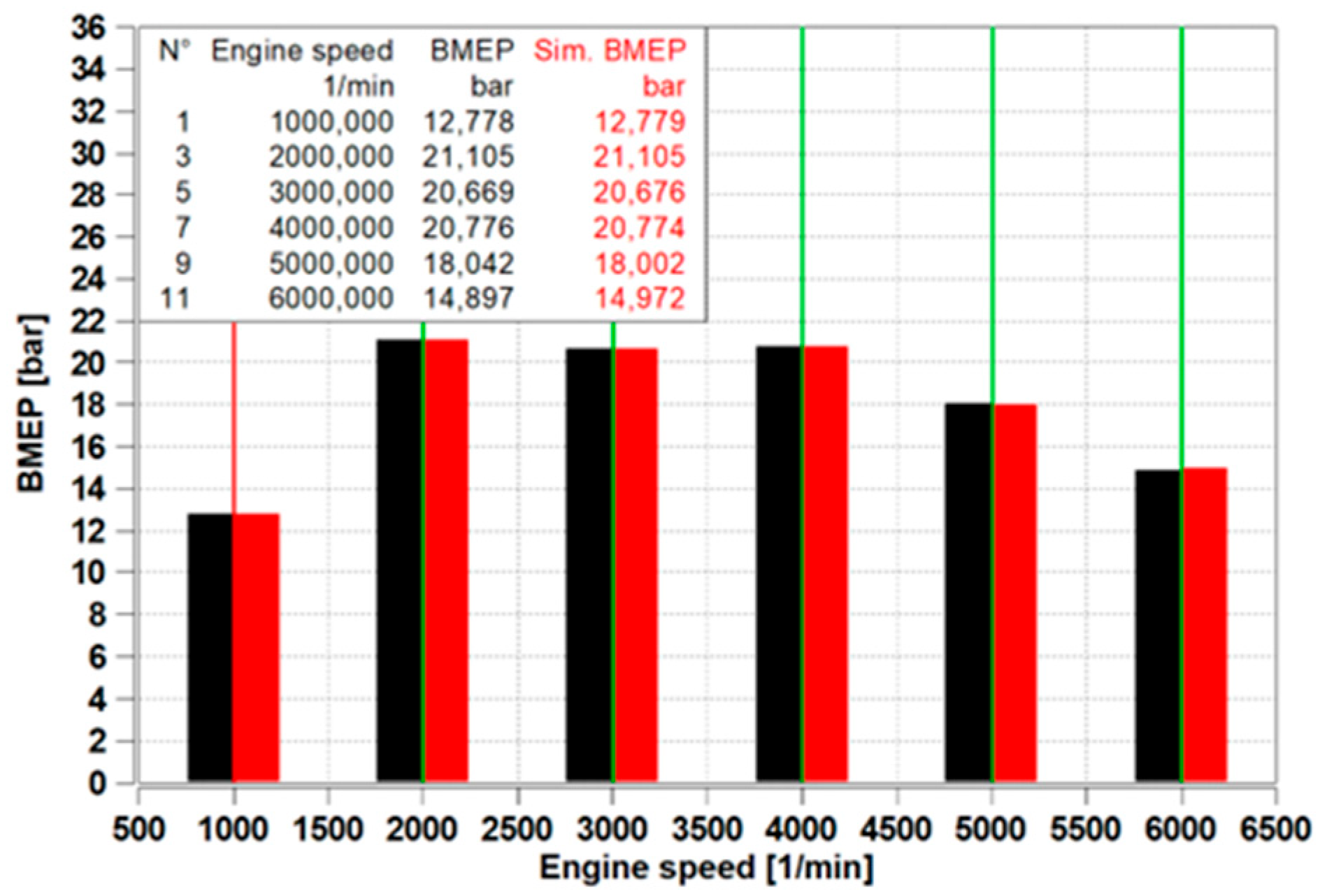
The values of the BMEP can be seen in Figure 3. The average absolute deviation was calculated to be 0.130%, indicating a high level of convergence between the simulation results and the experimental measurements.

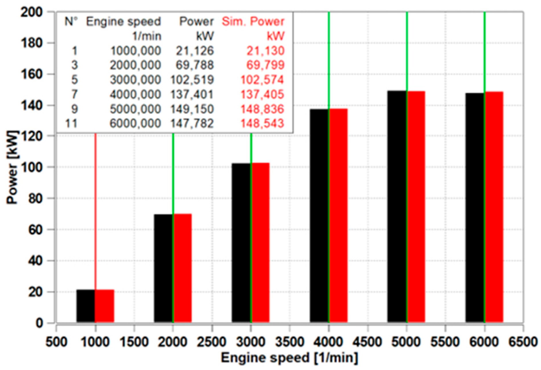
The measured and simulated engine power values are presented in Figure 4. The maximum deviation between the measured and simulated data is 0.515%, while the minimum deviation is 0.003%. The average deviation across all operating points is 0.136%, indicating a high level of agreement between the simulation results and experimental measurements.

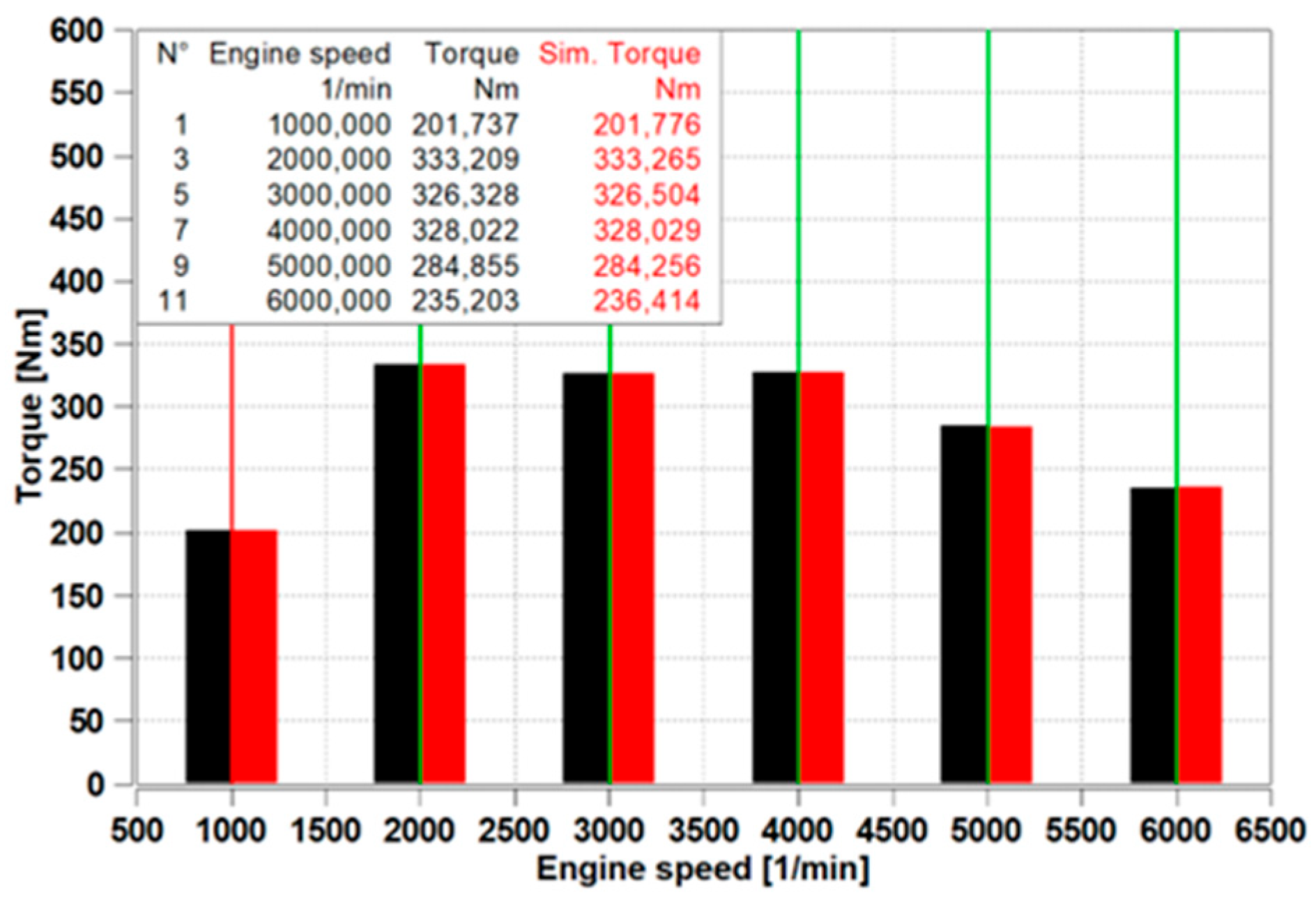
The torque values are shown in Figure 5 below. The maximum deviation is 0.515%, the minimum deviation is 0.002%, and the average deviation is 0.136%.

Power, torque, and BMEP are closely interrelated characteristics of internal combustion engines. There is a direct proportional relationship between torque and power—an increase in either torque or engine speed results in a higher power output [13]:

$$P=M_d·2\pi ·n$$

(1)

where

P = power [W];

M_d = torque [Nm];

n = engine speed [1/min].

BMEP (Brake Mean Effective Pressure) is a calculated parameter that represents the average pressure required within the engine cylinders to produce a given torque output. It serves as an indicator of how effectively the engine converts combustion pressure into mechanical work [13].

$$P_{me}={\displaystyle \frac{M_d·2\pi ·n}{V_{h}h·i}}$$

(2)

where

P_me = BMEP [Pa];

M_d = torque [Nm];

n = engine speed [1/min];

V_h = total swept volume of the engine [m³];

i = working cycles per revolution.

Due to the close interrelation of the parameters, the average deviation between simulation and measurement will be calculated by treating BMEP, power, and torque as single combined data.

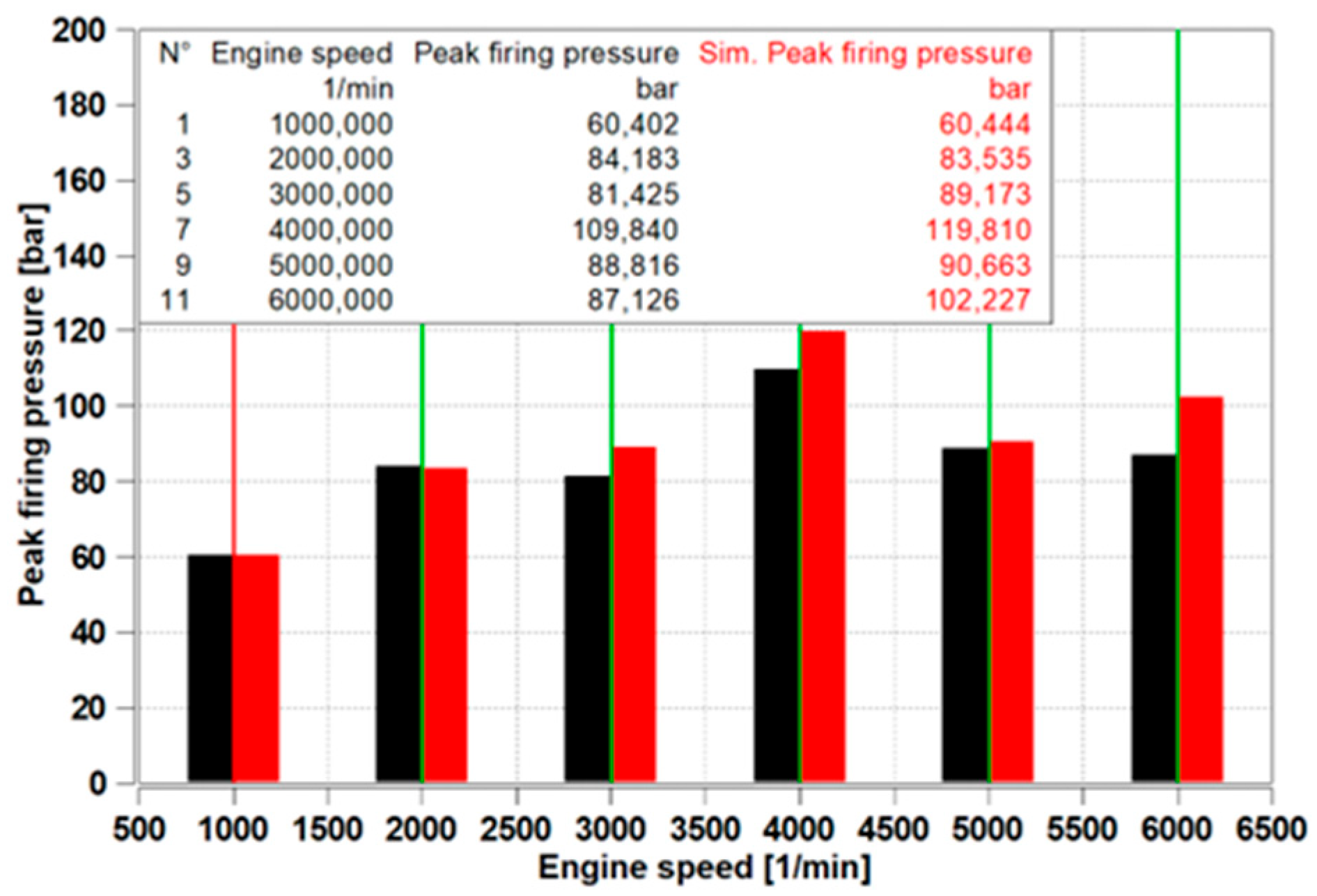
Figure 6 shows the peak firing pressures, measured with Kistler 6045B pressure sensor. The maximum deviation is 17.339%, and the minimum is 0.070%. The average deviation of the simulated peak firing pressure compared to the measured data is 6.475%.

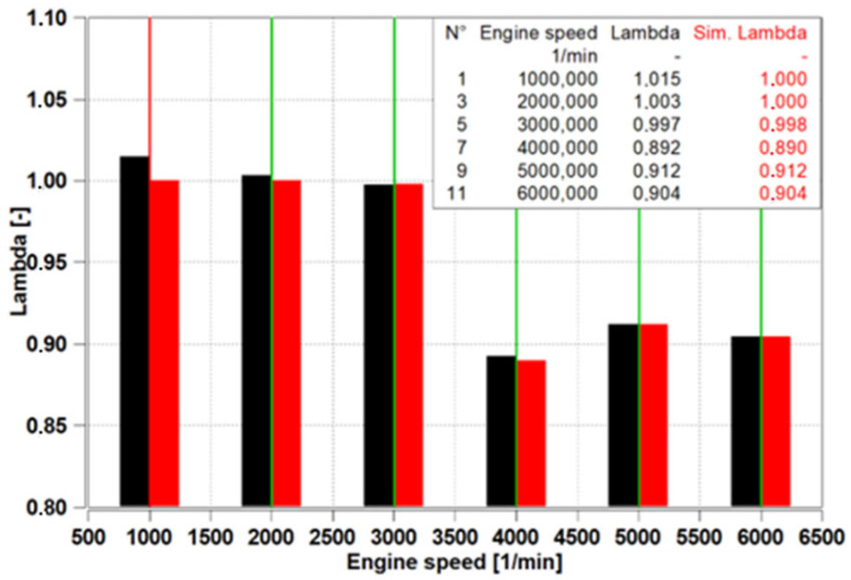
The air–fuel equivalence ratio can be seen in Figure 7. The maximum deviation observed is 1.479%, while the minimum is 0.000%. The average deviation across all operating points is 0.350%, indicating a high level of consistency between the simulation results and experimental measurements.

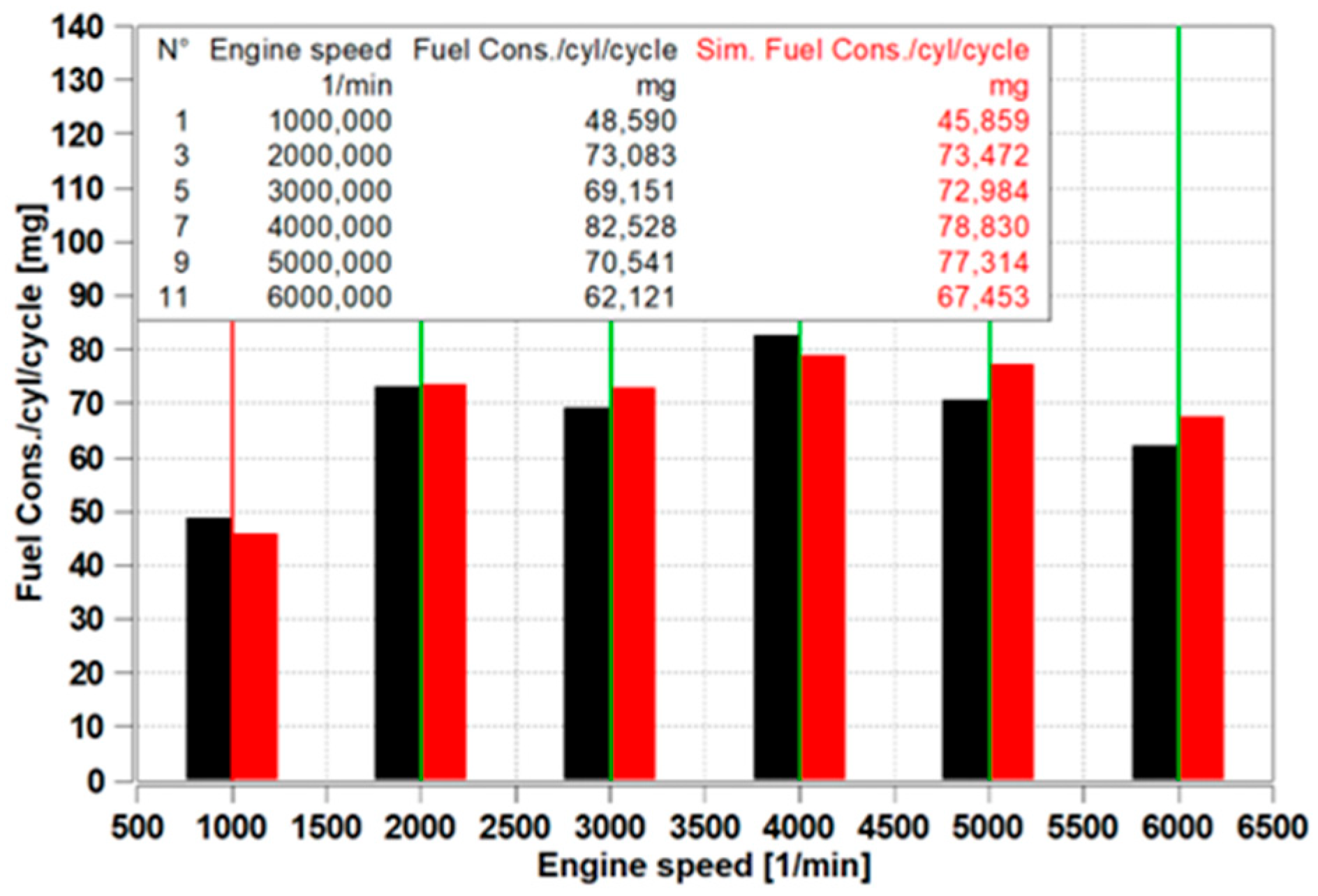
The fuel consumption trends across the operating points are illustrated in Figure 8. The maximum deviation between simulated and measured fuel consumption is 9.599%, while the minimum is 0.532%. The average deviation across all operating points is 5.730%, reflecting a moderate level of agreement between simulation and experimental results.

4. Conclusions

In the simulations conducted across six operating points, four out of the six evaluated parameters closely match the values measured on the engine test bench. Specifically, BMEP, power, torque, and the air–fuel equivalence ratio show deviations below 1%, indicating high accuracy. In contrast, peak combustion pressure and fuel consumption exhibit higher average deviations of 6.475% and 5.730%, respectively. The overall average deviation across all parameters is 3.173%, suggesting that the simulation model demonstrates sufficient accuracy for the evaluation of alternative fuels. However, additional simulation refinement is recommended to improve the accuracy of fuel consumption and peak firing pressure predictions.