Urban Mobility Modeling: Application to Seoul Bike-Sharing Data ^†

Abstract

This study applies a model from the normal variance–mean mixture family to capture daily demand in urban bike sharing. We fit both a mixture-based model and a standard Gaussian model to the logarithmic returns of total daily rental counts from the Seoul Bike-Sharing Demand dataset. Parameter estimation is performed, and model performance is assessed using mean squared error (MSE). Using one year of hourly rental data aggregated to daily counts from the Seoul Bike dataset, we find that the mixture-based model substantially outperforms the Gaussian counterpart, achieving a lower MSE. These results suggest that models from the normal variance–mean mixture family are more effective at capturing the large fluctuations and outliers inherent in bike-sharing demand data compared to models assuming normally distributed returns.

1. Introduction

Bike-sharing systems have been widely implemented across many countries as part of urban strategies to encourage sustainable transportation. In South Korea, the capital city of Seoul introduced its public bike-sharing program locally named Ddareungi and commonly referred to as Seoul Bike in 2015. The initiative aimed to alleviate urban issues such as increasing fuel costs, traffic congestion, and environmental pollution, while also encouraging a more active and healthier lifestyle for citizens. Initially launched along the Han River in October 2015, the program quickly expanded, with approximately 150 stations and 1500 bikes in operation within the first few months. By 2016, the system experienced substantial growth, eventually offering more than 20,000 bikes across Seoul. Today, with the aid of digital infrastructure, over 1500 rental stations operate city-wide, accessible 24/7 via mobile apps and internet-connected devices that provide real-time bike availability. Cycling has become a key urban transport mode due to safety concerns with public transit, changing travel patterns, and remote work. It supports sustainability by cutting emissions, improving health, and enhancing public transport integration [1,2]. Predicting cycling demand is crucial for effective planning and resource allocation, ensuring these systems meet urban mobility goals efficiently.

Given the scale and dynamic nature of Seoul’s bike-sharing program, accurate modeling of rental demand is essential for operational efficiency and policy planning. In this study, we apply a flexible probabilistic framework to model the daily variability in bike rental demand. Specifically, we focus on the logarithmic returns of daily rental counts, aggregated from hourly usage data in the Seoul Bike-Sharing Demand dataset. To capture the heavy tails and irregular fluctuations often observed in such demand patterns due to factors like weather, holidays, and local events, we employ a model from the normal variance–mean mixture family. This class of distributions generalizes the normal model by allowing for skewness and heavy tails, which are common in real-world data but inadequately captured by Gaussian assumptions [3].

We estimate the parameters of the mixture model using regression on quantiles, which provides a data-driven approach to identifying the structure of variability across different points in the distribution. Model performance is assessed by comparing the fitted series to a Gaussian benchmark using mean squared error (MSE). The results indicate that the mixture-based model yields a considerably better fit, effectively reflecting the variation and extremes observed in the daily demand series. These findings highlight the relevance of flexible, non-Gaussian modeling frameworks in transportation analytic, particularly those enhanced by machine learning and deep learning, as demonstrated in recent lead time prediction models developed for industrial systems [4], and deep anomaly detection methods using spatio-temporal clustering and congestion pattern analysis in urban mobility contexts [5].

The paper is divided into sections, with Section 2 providing an overview of the concepts of the variance–mean mixture framework and its statistical properties. Section 3 describes the dataset, preprocessing methods, estimation procedures, and empirical results. Finally, Section 4 concludes with a discussion of our findings and directions for future research.

2. The Normal Variance–Mean Mixture Model

Normal variance–mean mixture models provide a flexible framework for modeling data with skewness and heavy tails, extending the normal distribution by allowing its mean and variance to vary according to a latent mixing distribution. A prominent example within this class is the Normal Tempered Stable (NTS) model, introduced by [6]. The NTS model arises when the normal distribution is mixed with a tempered stable distribution, yielding a rich structure that can capture both asymmetry and heavy-tailed behavior. From a stochastic process perspective, it is equivalent to a Brownian motion modified by a tempered stable subordinator (for more details on tempered stable distributions (see [7,8,9,10,11,12]). Due to its flexibility and mathematical tractability, the NTS distribution has been successfully applied in a range of financial modeling tasks, as shown in the works of [3,13,14,15].

In essence, the tempered stable distribution is a variant of the stable distribution, adjusted through an exponential transformation, a concept presented by [6], page 3. Let us consider a tempered $\alpha$-stable random variable denoted as T, with $\alpha$ being the stability index in the range of (0,1). The Laplace transform of T is given for all values of $\theta$ less than ${\displaystyle \frac{{\gamma }^{\frac{1}{\alpha }}}{2}}$, as follows:

$$\mathbb{E}\left(e^{\theta T}\right)=exp\left[\delta \gamma \left(1-{\left(1-2{\gamma }^{-{\displaystyle \frac{1}{\alpha }}}\theta \right)}^{\alpha }\right)\right],$$

where $\delta >0$ and $\gamma >0$ (see [6] page 6). Without loss of generality, we take $\delta \gamma =1$ and we set $\lambda =2{\gamma }^{-{\displaystyle \frac{1}{\alpha }}}$. In what follows, we denote by ${\pi }_{\alpha ,\lambda }$ the distribution of T. Consider now a standard normal random variable $Z\sim N(0,1)$ independent of T. The normal tempered stable model describes the distribution of the random variable Y, which can be represented as $Y\stackrel{\mathbf{d}}{=}\sqrt{T}Z$, where $\stackrel{\mathbf{d}}{=}$ signifies equality in distribution. You can refer to [6] for further details on this concept, as mentioned on page 7 of their work. We denote by $f_{\alpha ,\lambda }$ the density function of Y. Please note that when y tends to $+\infty$, the density function $f_{\alpha ,\lambda }\left(y\right)$ has the following approximation:

$$f_{\alpha ,\lambda }\left(y\right)={\displaystyle \frac{e}{\sqrt{2\pi }}}{\int }_0^{+\infty }{\displaystyle \frac{e^{-\frac{y^2}{2x}}}{\sqrt{x}}}{\pi }_{\alpha ,\lambda }\left(dx\right)\sim c_{\alpha ,\lambda }{y}^{-\alpha -1}{e}^{-\sqrt{{\displaystyle \frac{2}{\lambda }}}y},$$

(1)

where ${\displaystyle c_{\alpha ,\lambda }=2^{\alpha +1}e{\left(2/\lambda \right)}^{-\frac{\alpha }{2}+\frac{1}{4}}\frac{\mathsf{\Gamma }(\alpha +1)}{\mathsf{\Gamma }\left(\alpha \right)\mathsf{\Gamma }(1-\alpha )}}$ (For more detail, we refer to [6] pages 7 and 8).

2.1. Estimation

In this section, we employ a novel parameter estimation method, which we have termed “the tail regression method”, for parameter estimation of $\alpha$ and $\lambda$ of the normal tempered stable model. This is achieved through the tail regression method, which is based on an approximation of the cumulative distribution of the response variable. This approximation establishes a linear relationship between certain transformations of the quantiles and the cumulative distribution function. The unknown parameters are then estimated using the least squares method.

We need first to approximate the Normal Tempered Stable distribution’s cumulative function, expressed as

$$F_Y\left(z\right)=\mathbf{P}(Y\le z)={\int }_{-\infty }^z{f}_{\alpha ,\lambda }\left(y\right)dy,\forall z\in \mathbf{R}.$$

The Equation (1) and the Hôpital’s rule imply that the survival function

$${\displaystyle {\overline{F}}_Y\left(z\right)=1-F_Y\left(z\right)\sim {\int }_z^{+\infty }{c}_{\alpha ,\lambda }{y}^{-\alpha -1}{e}^{-\sqrt{\frac{2}{\lambda }}y}dy,}$$

(2)

when $z\to +\infty$. By applying integration by parts, we obtain

$${\int }_z^{+\infty }{c}_{\alpha ,\lambda }{y}^{-\alpha -1}{e}^{-\sqrt{{\displaystyle \frac{2}{\lambda }}}y}dy=c_{\alpha ,\lambda }{z}^{-\alpha -1}\sqrt{{\displaystyle \frac{\lambda }{2}}}{e}^{-\sqrt{{\displaystyle \frac{2}{\lambda }}}z}-c_{\alpha ,\lambda }(\alpha +1)\sqrt{{\displaystyle \frac{\lambda }{2}}}{\int }_z^{+\infty }{y}^{-\alpha -2}{e}^{-\sqrt{{\displaystyle \frac{2}{\lambda }}}y}dy.$$

Let ${\displaystyle K\left(z\right)=\frac{(\alpha +1){\int }_z^{+\infty }{y}^{-\alpha -2}{e}^{-\sqrt{\frac{2}{\lambda }}y}dy}{z^{-\alpha -1}{e}^{-\sqrt{\frac{2}{\lambda }}z}}.}$ Since

$${\displaystyle 0\le {\int }_z^{+\infty }\frac{e^{-\sqrt{\frac{2}{\lambda }}y}}{y^{\alpha +2}}dy\le {\int }_z^{+\infty }\frac{e^{-\sqrt{\frac{2}{\lambda }}y}}{z^{\alpha +2}}dy=\frac{\sqrt{\frac{\lambda }{2}}{e}^{-\sqrt{\frac{2}{\lambda }}z}}{z^{\alpha +2}},}$$

then we obtain ${\displaystyle 0\le K\left(z\right)\le \sqrt{\frac{\lambda }{2}}{z}^{-1}.}$ This implies that ${\displaystyle K\left(z\right)⟶0, \mathrm{when} z\to +\infty .}$ Hence ${\displaystyle {\int }_z^{+\infty }{c}_{\alpha ,\lambda }{y}^{-\alpha -1}{e}^{-\sqrt{\frac{2}{\lambda }}y}dy\sim c_{\alpha ,\lambda }{z}^{-\alpha -1}\sqrt{\frac{\lambda }{2}}{e}^{-\sqrt{\frac{2}{\lambda }}z},}$ when $z\to +\infty .$ This, with (2), gives us the following approximation of the normal tempered stable cumulative function

$$F_Y\left(z\right)\sim 1-c_{\alpha ,\lambda }{z}^{-\alpha -1}\sqrt{{\displaystyle \frac{\lambda }{2}}}{e}^{-\sqrt{{\displaystyle \frac{2}{\lambda }}}z}, \mathrm{when} z\to +\infty .$$

(3)

Let $Y_1,Y_2,\dots ,Y_k$ be k copies of the normal tempered stable random variable Y and let $z_1,z_2,\dots ,z_n$ be n points on the tail of the empirical cumulative function. According to the law of large numbers, for k large enough, we have the following approximation ${\displaystyle f_i=\frac{1}{k}\sum _{j=1}^k{\mathbf{1}}_{\{Y_j>z_i\}}\sim {\overline{F}}_Y\left(z_i\right).}$ This together with (3) imply that for all $i\in \{1,2,\dots ,n\},$

$$ln\left(f_i\right)=ln\left(c_{\alpha ,\lambda }\sqrt{{\displaystyle \frac{\lambda }{2}}}\right)-\sqrt{{\displaystyle \frac{2}{\lambda }}}{z}_i-(\alpha +1)ln\left(z_i\right)+{\epsilon }_i,$$

where ${\epsilon }_i$ is a random error variable. This implies that the empirical mean of ${(ln\left(f_i\right))}_{1\le i\le n}$ is given by

$$\overline{ln\left(f\right)}=ln\left(c_{\alpha ,\lambda }\sqrt{{\displaystyle \frac{\lambda }{2}}}\right)-\sqrt{{\displaystyle \frac{2}{\lambda }}}\overline{z}-(\alpha +1)\overline{ln\left(z\right)}+\overline{\epsilon },$$

where ${\displaystyle \overline{ln\left(f\right)}=\frac{1}{n}\sum _{i=1}^{n}ln\left(f_i\right)}$, ${\displaystyle \overline{z}=\frac{1}{n}\sum _{i=1}^n{z}_i}$, ${\displaystyle \overline{ln\left(z\right)}=\frac{1}{n}\sum _{i=1}^{n}ln\left(z_i\right)}$ and ${\displaystyle \overline{\epsilon }=\frac{1}{n}\sum _{i=1}^n{\epsilon }_i.}$ Therefore

$$ln\left(f_i\right)-\overline{ln\left(f\right)}=-\sqrt{{\displaystyle \frac{2}{\lambda }}}(z_i-\overline{z})-(\alpha +1)(ln\left(z_i\right)-\overline{ln\left(z\right)})+({\epsilon }_i-\overline{\epsilon }),$$

for all $i\in \{1,2,\dots ,n\}.$ Let $\mathbf{X}=\left(\begin{array}{cc}ln\left(z_1\right)-\overline{ln\left(z\right)}& z_1-\overline{z}\\ ln\left(z_2\right)-\overline{ln\left(z\right)}& z_2-\overline{z}\\ ⋮& ⋮\\ ln\left(z_n\right)-\overline{ln\left(z\right)}& z_n-\overline{z}\end{array}\right)$, $\mathbf{Y}=\left(\begin{array}{c}ln\left(f_1\right)-\overline{ln\left(f\right)}\\ ⋮\\ ln\left(f_n\right)-\overline{ln\left(f\right)}\end{array}\right)$, $ϵ=\left(\begin{array}{c}{\epsilon }_1-\overline{\epsilon }\\ ⋮\\ {\epsilon }_n-\overline{\epsilon }\end{array}\right)$ and $\theta =\left(\begin{array}{c}-\alpha -1\\ -\sqrt{2/\lambda }\end{array}\right)$, we obtain the following linear regression model

$$\mathbf{Y}=\mathbf{X}\theta +ϵ.$$

Using the least squares method (For more details about this method, please see [12], Page 155), we deduce that the estimator ${\displaystyle \widehat{\theta }={\left({\mathbf{X}}^T\mathbf{X}\right)}^{-1}{\mathbf{X}}^T\mathbf{Y},}$ where ${\mathbf{X}}^T$ is the transpose matrix of $\mathbf{X}.$ Since $\theta =\left(\begin{array}{c}-\alpha -1\\ -\sqrt{2/\lambda }\end{array}\right)$, then by projecting $\theta$ on the canonical basis $e_1=(1,0)$ and $e_2=(0,1)$ of ${\mathbf{R}}^2$, we obtain $\langle \theta ,e_1\rangle =-\alpha -1$ and $\langle \theta ,e_2\rangle =-\sqrt{2/\lambda }$. It follows that the estimators $\widehat{\alpha }$ and $\widehat{\lambda }$ of $\alpha$ and $\lambda$ are given by

$${\displaystyle \widehat{\alpha }=-\langle \widehat{\theta },e_1\rangle -1, \mathrm{and} \widehat{\lambda }=\frac{2}{{\langle \widehat{\theta },e_2\rangle }^2}.}$$

2.2. Numerical Illustration

In this section, we present an algorithm for simulating the normal tempered stable model and provide a numerical demonstration of the estimated parameters $\alpha$ and $\lambda$.

Our approach begins with simulating the standard stable distribution, as outlined by [16], page 20, which allows us to approximate the density of the standard stable model. Given that the tempered stable distribution can be viewed as a stable distribution altered through exponential tempering (as indicated in the work of [6], page 3), we proceed to approximate the density of the tempered stable model. Using this approximation, we derive an estimate of the cumulative distribution function for the tempered stable distribution. By employing the inverse transform sampling method, we generate simulations of the tempered stable model. Figure 1 provides a visual depiction of the tempered stable distribution curves, showcasing various values of $\alpha$ and $\lambda$.

Suppose we have a set of n independent observations from the tempered stable distribution, denoted as $x_1,x_2,\dots ,x_n$. Utilizing the Monte Carlo integration technique (for a comprehensive understanding of this method, refer to [17]) and the expression for the normal tempered stable density provided in Equation (1), we obtain the following result:

$$f_{\alpha ,\lambda }\left(y\right)=\underset{n\to +\infty }{lim}{\displaystyle \frac{1}{n}}\sum _{i=1}^n{\displaystyle \frac{e}{\sqrt{2\pi x_i}}}{e}^{-{\displaystyle \frac{y^2}{2x_i}}}.$$

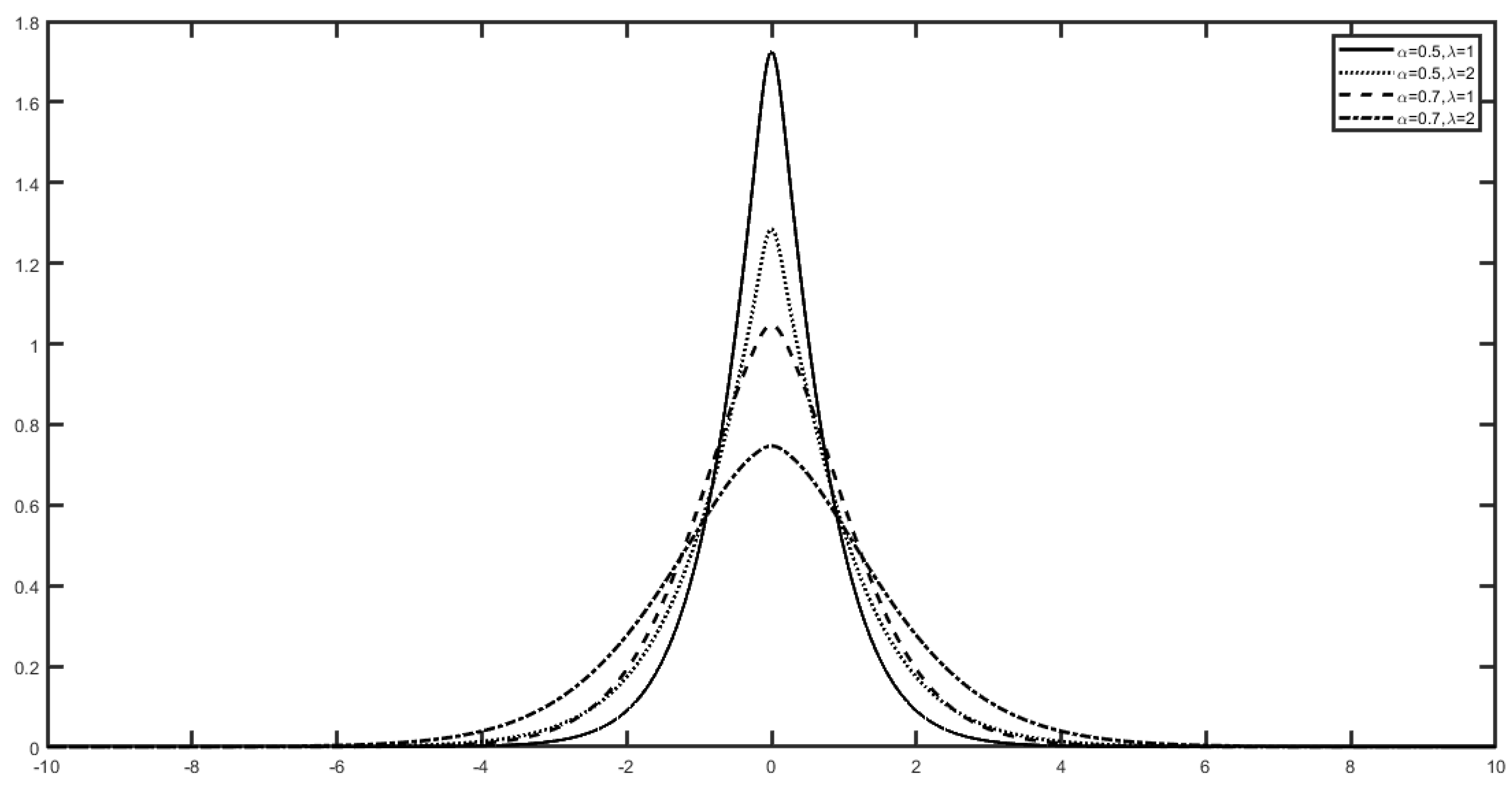
As a result, the application of the method of the inverse transform sampling enables us to generate simulations as desired. Figure 2 illustrates the curves of the normal tempered stable distribution, showcasing various combinations of $\alpha$ and $\lambda$ values.

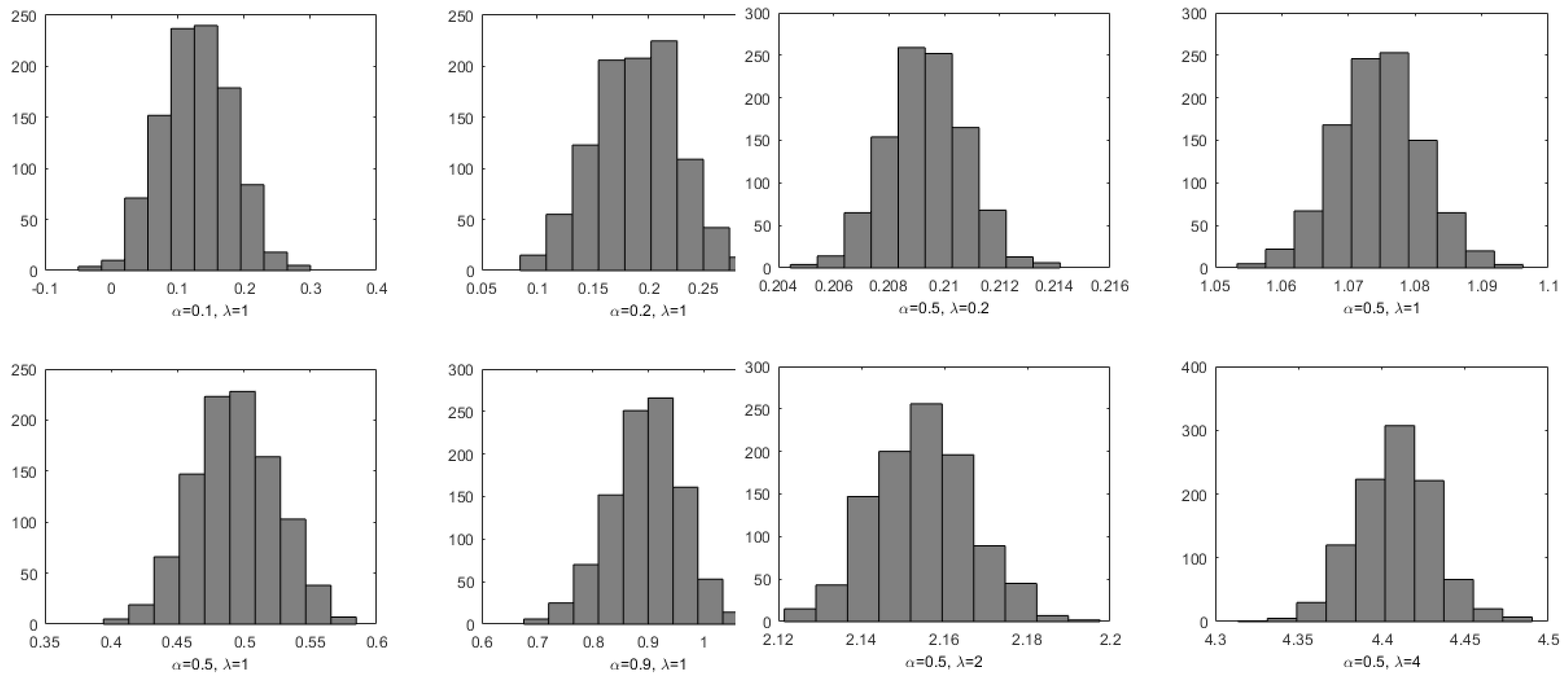
Next, we proceed to generate a dataset of 1000 observations from the normal tempered stable distribution. Subsequently, we select 1000 data points from the upper tail of the empirical cumulative distribution function, ensuring that they satisfy the condition $F_Y\left(z_i\right)>0.8$, where i ranges from 1 to 1000. The estimation of $\widehat{\theta }$ leads us to determine the ones of $\widehat{\alpha }$ and $\widehat{\lambda }$. Then, we compute the estimators $\widehat{\alpha }$ and $\widehat{\lambda }$, and we consider 1000 samples of these estimators. Figure 3 represents the histograms of the estimators $\widehat{\alpha }$ and $\widehat{\lambda }$.

It is worth noting that the histograms of the estimators, $\widehat{\alpha }$ and $\widehat{\lambda }$, exhibit a normal distribution-like shape. To assess the performance of the estimated parameters, $\widehat{\alpha }$ and $\widehat{\lambda }$, we employ the mean squared error (MSE), defined as: ${\displaystyle MSE\left(\widehat{\alpha }\right)=\frac{1}{K}\sum _{i=1}^K{({\widehat{\alpha }}_i-\alpha )}^2}$ and ${\displaystyle MSE\left(\widehat{\lambda }\right)=\frac{1}{K}\sum _{i=1}^K{({\widehat{\lambda }}_i-\lambda )}^2,}$ We also calculate their coefficients of variation (CV), defined as:

$${\displaystyle CV\left(\widehat{\alpha }\right)=\frac{\sqrt{MSE\left(\widehat{\alpha }\right)}}{mean\left(\widehat{\alpha }\right)} \mathrm{and} CV\left(\widehat{\lambda }\right)=\frac{\sqrt{MSE\left(\widehat{\lambda }\right)}}{mean\left(\widehat{\lambda }\right)},}$$

where ${\displaystyle mean\left(\widehat{\alpha }\right)=\frac{1}{K}\sum _{i=1}^K{\widehat{\alpha }}_i}$ and ${\displaystyle mean\left(\widehat{\lambda }\right)=\frac{1}{K}\sum _{i=1}^K{\widehat{\lambda }}_i.}$ The results of our simulations are given in

Table 1. An examination of the estimators $\widehat{\alpha }$ and $\widehat{\lambda }$, along with their mean squared errors (MSEs) and coefficient of variations (CVs).

$\mathit{\alpha }$	$\mathit{\lambda }$	$\widehat{\mathit{\alpha }}$	$\widehat{\mathit{\lambda }}$	$\mathit{MSE}\left(\widehat{\mathit{\alpha }}\right)$	$\mathit{MSE}\left(\widehat{\mathit{\lambda }}\right)$	$\mathit{CV}\left(\widehat{\mathit{\alpha }}\right)$	$\mathit{CV}\left(\widehat{\mathit{\lambda }}\right)$
$0.2$	1	$0.1875$	$1.0699$	$0.0016$	$0.0049$	$0.2147$	$0.0653$
$0.2$	2	$0.1468$	$2.1259$	$0.0041$	$0.0162$	$0.4412$	$0.0598$
$0.5$	1	$0.4951$	$1.0745$	$0.0010$	$0.0056$	$0.0630$	$0.0698$
$0.5$	2	$0.4626$	$2.1551$	$0.0022$	$0.0240$	$0.1031$	$0.0719$
$0.7$	1	$0.6876$	$1.0340$	$0.0015$	$0.0012$	$0.0534$	$0.0336$
$0.7$	2	$0.6707$	$2.0912$	$0.0018$	$0.0086$	$0.0638$	$0.0440$

.

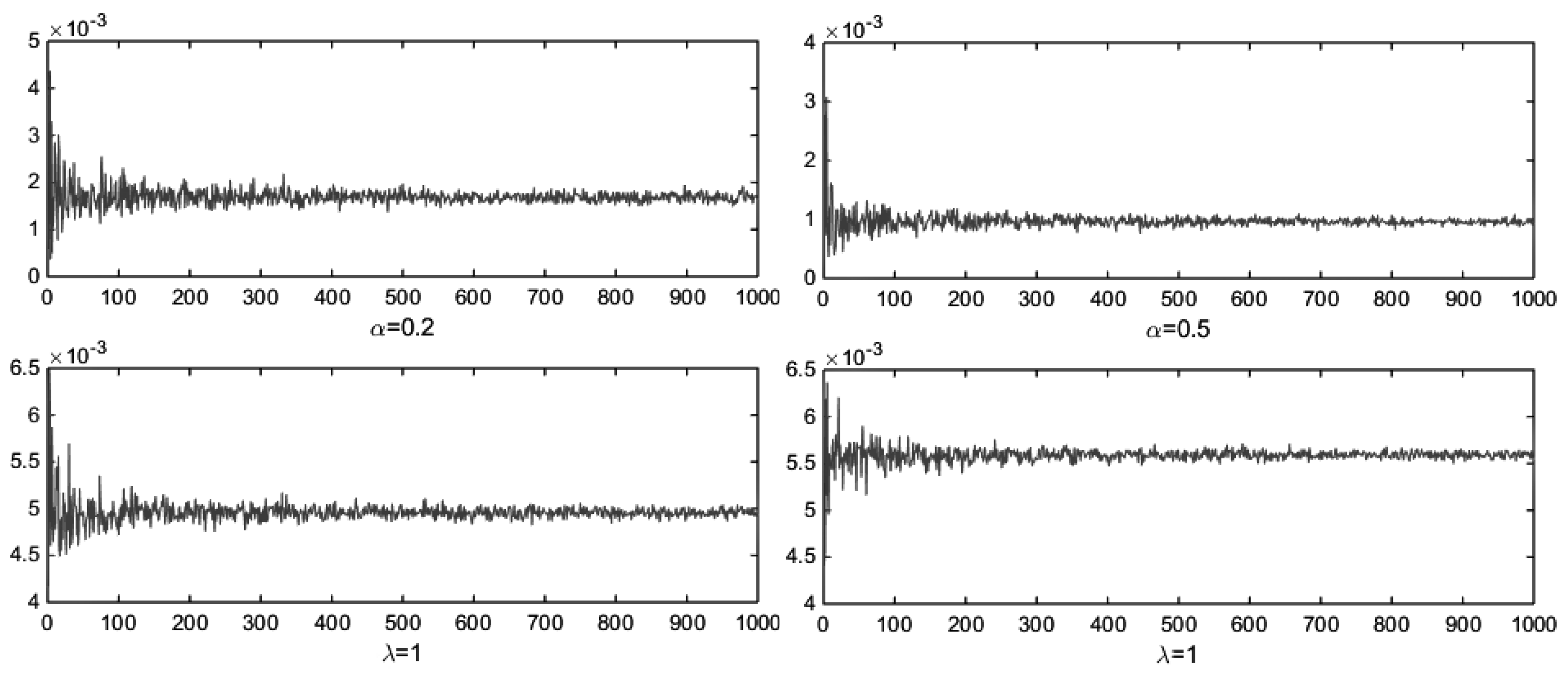
Subsequently, we present the plots depicting the mean squared errors (MSEs) of $\widehat{\alpha }$ and $\widehat{\lambda }$ under two scenarios: one with $\alpha =0.2$ and $\lambda =1$, and the other with $\alpha =0.5$ and $\lambda =1$.

From the data presented in Figure 4, we observe that the mean squared error for $\alpha$ remains below $5\times {10}^{-3}$ for the case of $\alpha =0.2; \lambda =1$, and below $4\times {10}^{-3}$ for $\alpha =0.5; \lambda =1$. Additionally, the mean squared error for $\lambda$ is less than $6.5\times {10}^{-3}$.

3. Modeling Bike-Sharing Data

The dataset comprises the count of total rental bikes in Seoul [18]. To facilitate our analysis, we introduce this Log Return transformation

$${\displaystyle S_i=log(R_i/R_{i-1}),}$$

where $R_i$ is the count of total rental bikes in day i Based on the data $S_i$, we utilize the tailed regression model to estimate the parameters $\alpha$ and $\lambda$ of the normal tempered stable law. Additionally, to facilitate a comparison with the normal distribution, we perform parameter estimation for the normal distribution, namely the mean $\mu$ and the variance ${\sigma }^2$, using the same dataset. The results of our estimations are summarized in

Table 2. Estimating the parameters for the Log Return data by utilizing both the normal and normal tempered stable models.

$\mathbf{Parameters}$	$\widehat{\mathit{\mu }}$	$\widehat{{\mathit{\sigma }}^2}$	$\widehat{\mathit{\alpha }}$	$\widehat{\mathit{\lambda }}$
$\mathrm{Normal}\mathrm{model}$	$-1.1504\times {10}^{-4}$	$0.4253$	−	−
$\mathrm{Normal}\mathrm{tempered}\mathrm{stable}\mathrm{model}$	−	−	$0.4558$	$0.3968$

:

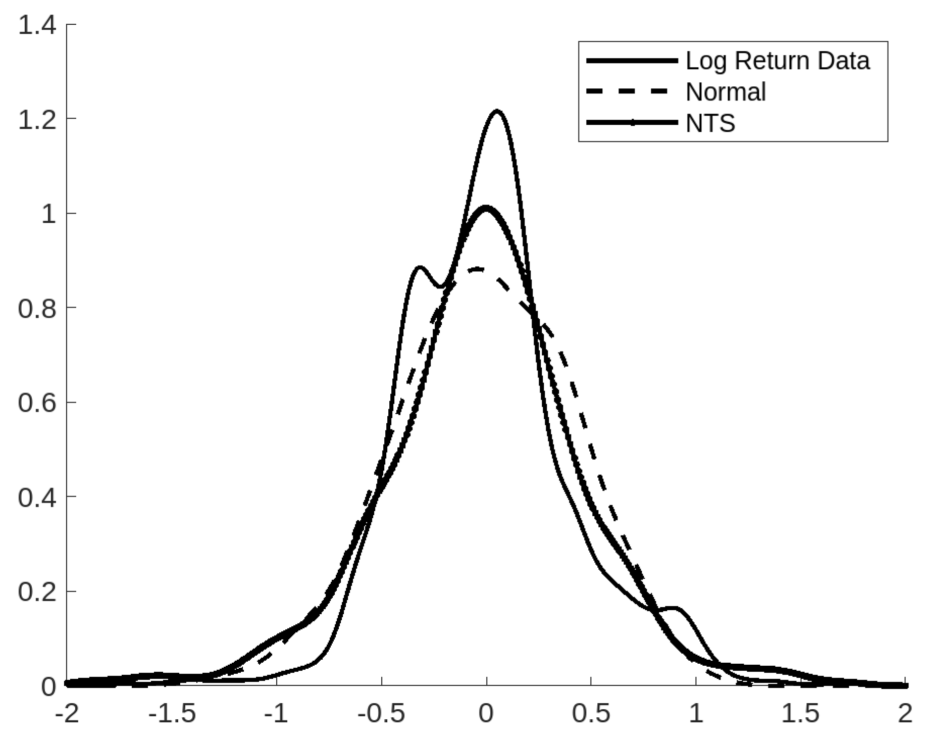
To enable a meaningful comparison between the dataset and the simulated normal distribution (characterized by estimated parameters $\widehat{\mu }$ and $\widehat{{\sigma }^2}$), as well as the simulated normal tempered stable distribution (with estimated parameters $\widehat{\alpha }$ and $\widehat{\lambda }$), we provide the following visual representation. This Figure 5 illustrates the curves corresponding to the dataset, the simulated normal tempered stable distribution, and the simulated normal distribution.

In order to compute the errors between the simulated models and the data, we calculate the Mean Squared Error (MSE) in

Table 3. MSE between the Log return data and the normal distribution, and the normal tempered stable distribution.

	Normal Model	Normal Tempered Stable Model
MSE	0.013002	0.0076658

to quantify the errors between the simulations and the actual data:

Based on the analysis of Table 3, it can be inferred that the normal tempered stable (NTS) model outperforms the normal distribution in handling the Log Return data. Therefore, by employing a simulation of the NTS distribution denoted as $S_{NTS}$, we can substitute the Log Return values with the simulated values from $S_{NTS}$. This presents us with the chance to establish the relationship between $R_i$ and $R_{i-1}$ in both directions. Specifically, we have the following relations:

$$R_i=R_{i-1}exp\left(S_i\right)\approx R_{i-1}exp\left(S_{NTS}\right)$$

4. Conclusions

This paper introduces the Normal Tempered Stable (NTS) distribution for modeling daily bike-sharing demand, offering a robust alternative to Gaussian models by capturing heavy-tailed fluctuations and volatility. We derive its theoretical properties for demand log-returns and propose a novel tail-regression estimation method. Empirical tests on Seoul Bike-Sharing data show the NTS model outperforms Gaussian models in forecasting accuracy, particularly for extreme demand spikes. Key advantages include improved mean squared error (MSE) and better volatility prediction. Future work may extend the model to hourly demand, integrate weather/demographic factors, and test it across other cities and transport modes to enhance generalizability.

References

1. El Amrani, A.M.; Fri, M.; Benmoussa, O.; Rouky, N. The integration of urban freight in public transportation: A systematic literature review. Sustainability 2024, 16, 5286. [Google Scholar] [CrossRef]
2. Benjdiya, O.; Rouky, N.; Benmoussa, O.; Fri, M. On the use of machine learning techniques and discrete choice models in mode choice analysis. LogForum 2023, 19, 321–336. [Google Scholar] [CrossRef]
3. Charfi, S.; Mselmi, F. Modeling exchange rate volatility: Application of GARCH models with a Normal Tempered Stable distribution. Quant. Financ. Econ. 2022, 6, 206–222. [Google Scholar] [CrossRef]
4. Fri, M. Lead time prediction using advanced deep learning approaches: A case study in the textile industry. LogForum 2024, 20, 145–155. [Google Scholar] [CrossRef]
5. Oucheikh, R.; Fri, M.; Fedouaki, F.; Hain, M. Deep anomaly detector based on spatio-temporal clustering for connected autonomous vehicles. In Proceedings of the International Conference on Ad Hoc Networks, Paris, France, 17 November 2020; pp. 201–212. [Google Scholar]
6. Barndorff-Nielsen, O.E.; Shephard, N. Normal modified stable processes. Theor. Probab. Math. Stat. 2001, 65, 1–19. [Google Scholar]
7. Bianchi, M.L.; Tassinari, G.L. Estimation for multivariate normal rapidly decreasing tempered stable distributions. J. Stat. Comput. Simul. 2024, 94, 103–125. [Google Scholar] [CrossRef]
8. Xia, Y.; Grabchak, M. Estimation and simulation for multivariate tempered stable distributions. J. Stat. Comput. Simul. 2022, 92, 451–475. [Google Scholar] [CrossRef]
9. Baeumer, B.; Kovács, M. Approximating multivariate tempered stable processes. J. Appl. Probab. 2012, 49, 167–183. [Google Scholar] [CrossRef]
10. Mselmi, F. Lévy processes time-changed by the first-exit time of the inverse Gaussian subordinator. Filomat 2018, 32, 2545–2552. [Google Scholar] [CrossRef]
11. Mselmi, F. Characterization of the inverse stable subordinator. Stat. Probab. Lett. 2018, 140, 37–43. [Google Scholar] [CrossRef]
12. Rencher, A.C.; Christensen, W.F. Methods of Multivariate Analysis; John Wiley & Sons: Hoboken, NJ, USA, 2012. [Google Scholar]
13. Bianchi, M.L.; Tassinari, G.L.; Fabozzi, F.J. Riding with the four horsemen and the multivariate normal tempered stable model. Int. J. Theor. Appl. Financ. 2016, 19, 1650027. [Google Scholar] [CrossRef]
14. Sabino, P. Normal tempered stable processes and the pricing of energy derivatives. SIAM J. Financ. Math. 2023, 14, 99–126. [Google Scholar] [CrossRef]
15. Sabino, P. Exact simulation of normal tempered stable processes of OU type with applications. Stat. Comput. 2022, 32, 81. [Google Scholar] [CrossRef]
16. Nolan, J.P. Stable Distributions: Models for Heavy Tailed Data; Birkhäuser: Boston, MA, USA, 2008. [Google Scholar]
17. Geweke, J. Monte Carlo simulation and numerical integration. Handb. Comput. Econ. 1996, 1, 731–800. [Google Scholar]
18. UCI Machine Learning Repository. Bike Sharing. Available online: https://archive.ics.uci.edu/dataset/275/bike+sharing+dataset (accessed on 25 June 2025).
Figure 1. Curves of the tempered stable distribution for different values of α and λ .
Engproc 112 00051 g001
Figure 2. Curves of the normal tempered stable distribution for different values of α and λ .
Engproc 112 00051 g002
Figure 3. Histograms of α ^ and λ ^ .
Engproc 112 00051 g003
Figure 4. Curves of the M S E ( α ^ ) and M S E ( λ ^ ) when { α = 0.2 ,   λ = 1 } and { α = 0.5 ,   λ = 1 } .
Engproc 112 00051 g004
Figure 5. The curve of the Log Return data compared with the simulated normal tempered stable distribution, and the simulated normal distribution.
Engproc 112 00051 g005