Fire Detection Using CCTV Images with 1-Dimensional Convolutional Neural Network Based on GUI ^†

Abstract

Fire is a phenomenon that causes physical and material losses to humans. Fires are difficult to predict based on causes and location. Therefore, early detection of fires is necessary to reduce the impact. With these issues, this research aims to detect fires based on CCTV images. So far, there has been no research on fire detection based on CCTV images using a 1D CNN. The detection of fires based on CCTV images will be carried out by creating an algorithm model with a 1D convolutional neural network. This research uses a dataset of fire images based on CCTV that is already pre-processed. An interface display is created for inputting data using the Tkinter library to show a graphical user interface (GUI). The result of the algorithm model process using the 1D convolutional neural network based on accuracy, precision, and recall is 88.43%. The understanding of the actual input data is still low in terms of detecting fires based on CCTV images and requires further processing of CCTV image data.

1. Introduction

Fire is a non-natural disaster that can occur in various places, such as forests, land, or buildings in densely populated residential areas. According to DKI Regional Regulation Number 3 of 1992, a fire is an event or occurrence of fire that cannot be controlled, which is dangerous and threatens the safety of life and property. The general definition of fire according to the National Disaster Management Agency (BNPB) is a situation where houses, buildings, etc., are hit by a fire that can have a number of victims and/or cause significant losses. Then, in general, it can be known and concluded that this fire is a phenomenon of the emergence of hotspots in a particular building that cannot be controlled and causes a number of significant losses for the victims.

Fires that occur cannot be predicted in advance with regard to where and exactly when they will occur. Fires can appear suddenly in places that are difficult to predict due to the many supporting factors that can cause a fire to occur. One of the common factors that cause a fire to occur in a building is an electrical short circuit, which triggers the appearance of sparks that hit a flammable object [1]. Electrical short circuits occur due to poor electrical installation and the use of inappropriate electrical equipment. Apart from electrical short circuits, cooking equipment that is often used is also a main factor causing fires due to low vigilance and negligence in its use. Apart from that, there is a lack of proper education regarding fire prevention measures in the community so that if there is a potential fire, the community can handle it with appropriate steps.

Having appropriate treatment and prevention to reduce the impact of the occurrence of a fire is an important action. Applying technology to reduce the risk of fire can also help reduce the impact of and the potential for a fire to occur. A closed-circuit television (CCTV) camera is a surveillance system that is connected to a device to monitor and record certain activities and certain locations. CCTV cameras can record and monitor what happens as long as the cameras are active.

Research regarding processing an image to predict the presence of fire in the image was carried out by Zaky Farhan Abror in 2019. In this research, image processing used a CNN (convolutional neural network) algorithm, which was processed in two dimensions. In the image processing carried out, the researcher did not change the color levels in the image and continued to use the original RGB (Red, Green, Blue) image values with a pixel size of 150 × 150 pixels. The results obtained in this research can be said to be good, with an accuracy of 98.8% in predicting a fire image [2].

Apart from that, other previous research was carried out by Muh Amin Faiz Nur Ridho and coworkers. The research focused on predicting fire areas based on temperature levels in an area using a linear regression algorithm. This research produced an RMSE (Root Mean Squared Error) metric score level of 63%, which indicates that the linear regression model is not good enough in the process of predicting area results [3].

There are a number of other modeling algorithm methods that can be used in creating image-based fire prediction programs. The level of effectiveness of a modeling algorithm in detecting and predicting an existing pattern depends on using the right data and processing it well. The model will learn from the data to become intelligent so that it can find the best patterns in detecting existing input data. One of the popular algorithms in image detection is CNN (convolutional neural network), which can easily understand data patterns by performing a small amount of processing on the image object [4]. However, CNNs not only carry out the learning process with two-dimensional data but also with tabular input data in one dimension. This is because a CNN is a neural-based deep learning algorithm or artificial neural network that has a number of layers to detect and learn input data.

Therefore, this research will focus on using the one-dimensional CNN algorithm to carry out a tabular-based classification process for input data. The reason for changing the dimensions of the CNN, which was originally two-dimensional, to one-dimensional is that in the image data feature extraction process, the results obtained will be in the form of one-dimensional tabular data after going through a number of extraction calculation processes. The learning process of the CNN model is expected to be able to classify fire image data based on CCTV images well.

2. Methods

2.1. Research Process Stages

To achieve a research objective, the researcher provides a general description of the flow from the preparation of this research to completion. A general overview of the research stages can be seen in Figure 1.

2.2. Data Pre-Processing

Data pre-processing can minimize the occurrence of errors resulting from inconsistencies in the data entered into the machine learning model. From a number of existing literature reviews, researchers will use a number of methods for the required data pre-processing stages, namely image sharpening, color segmentation, feature extraction, target encoder, target balancing, and split train testing, as can be seen in Figure 2.

In the initial stage of data pre-processing, researchers sharpen the image quality of the image itself. The image sharpening process that researchers will use is the Gaussian Blur process which comes from the built-in OpenCV library. In this process, the image that previously looked blurry will be changed to be sharper in terms of color to further emphasize the colors that will be analyzed in the image segmentation process later.

Images that have undergone a sharpening process will undergo a color segmentation process. The colors that will be looked for to detect the color of fire are red, orange and also white. In the color masking process in the image, the number of values in the area detected in the existing color masking will be determined. The results of the red, orange and white color values detected in the masking will be entered into the data frame for the classification process or detection of whether there is fire in the existing input image.

Researchers carry out a feature extraction process on image datasets to obtain CCTV image data patterns that will be used in training and prediction. The purpose of this feature extraction process is that the machine learning model can find all feature information that is present in detection and prediction [5]. Researchers use the GLCM (Gray Level Co-occurrence Matrix) process to extract features in the image, which changes the image to a gray image.

Features that will be used as a reference for training and predicting data will be in string format. This value must be changed to a number format because the machine learning model cannot read targets in string format properly. This must be performed to make it easier for the model to train. This encoder can be used using the label encoder process to change the target value into a number format with a unique value according to the number of target types available [6].

The division between training data and test data must be performed to make the machine learning model easier in the training process. In general, the division of training data and test data can be performed with a composition of 80% training data and 20% test data. However, this is flexible according to the size of the data and the needs of the researcher. The machine learning model will learn with training data and the learning results will be tested with test data that has been prepared and shared previously.

2.3. Modeling 1-Dimensional CNN

Data that is clean and has been pre-processed beforehand is ready for the modeling process. The data will enter the neural network processing environment with the One-Dimensional Convolutional Neural Network algorithm for the learning process. The architectural layers of a One-Dimensional Convolutional Neural Network have convolution, pooling, and connected layers. The preparation of the convolution layer is adjusted based on a number of best experiments on the characteristics of the input fire data so that important patterns can be identified by the algorithm model for learning.

The pooling layer is placed after the convolution layer, which indicates that the results of the convolution will be searched for the largest pixels using the max pooling process. The placement of pooling after the convolution process aims to reduce the dimensions of the data so that we can better understand the important features in the input data based on the pixel values. This process can also minimize the computational process in the learning process because the dimensions of the input data are minimized without eliminating important features.

The connected layer is arranged in this research as the final layer in the architectural process before the algorithm model produces a prediction output for fire input data. The number of connected layers used in this research will be more than 1 connected layer. This is because in the process of learning and training algorithm models, there needs to be a variety of possible patterns, so that we can obtain appropriate data learning patterns with appropriate weight values.

2.4. Model Evaluation

The evaluation results of the algorithm model learning process on existing fire input data were analyzed to find out how well the model was able to carry out the prediction process and understand existing data patterns. The researchers used a classification evaluation method to measure the value of the accuracy metric. The accuracy results obtained will be compared with the actual data validation results in each running epoch so that the distribution of accuracy values of the algorithm model making predictions and detections can be known. The researchers use accuracy metrics measurement values because they want to focus on the level of suitability of existing prediction results. In addition, measurements using metric value evaluation with accuracy can be better understood in the interpretation of results. A simple example is that if the accuracy metric result is 80%, then the algorithm model only correctly predicts 80% of the total available fire data as input fire data. Moreover, by default with the TensorFlow library system, the accuracy metric is the default measurement parameter system so it can be more easily accessed.

2.5. GUI Development Process

After knowing the results of the performance of the algorithm model based on the level of values of the metrics used, the next step is to create a graphical user interface (GUI). Creating a GUI makes it easier for users to interact with and use algorithm models to carry out the detection process [7]. The algorithm model that has been prepared and evaluated previously will be exported into a modeling file format. The algorithm model file will be called and used in preparing the interface for the user.

The GUI is created based on research needs and structure. This research will use an algorithm model that functions with types of fire datasets based on CCTV images. So, the main page will be arranged containing 2 choices of button types regarding detection. After the user enters the required data, detection results will appear according to the input data entered.

3. Results and Discussion

3.1. Data Gathering

The data used is a dataset that comes from an open-source site, namely Kaggle. In this research, researchers used fire data based on CCTV images. Kaggle provides various datasets needed by users according to their needs. Fire data based on CCTV images is downloaded from the Kaggle site with a size of 341MB and has a total data sample of 841 samples in the train and test folders and has 3 classes, namely the default, fire and smoke classes (Figure 3).

3.2. Exploratory Data Analysis

In the fire dataset based on CCTV images, it is known that the images used have various conditions captured by CCTV cameras; for example, there are images captured from CCTV cameras in a house, a room, and even on a freeway. From the checking process, it is known that the size of each CCTV image is 224 × 224 pixels. It can also be seen that CCTV images have three channel layers which represent RGB (Red Green Blue) values. It can be seen that there are a number of images that do not match the type of label of the image itself, so the images that do not match can be removed from the dataset. In total, there were previously 841 images, and after deletions, there are 601 final images that will be used from the three existing types of class targets. To understand the characteristics of image data, it can be converted into gray format which has one channel so that the processes of extracting texture features and modeling in one dimension can be carried out using GLCM (Gray Level Co-occurrence Matrix), which was previously used in the color segmentation processes of the image to obtain the expected value of the color in the image.

3.3. The Result of Data Pre-Processing

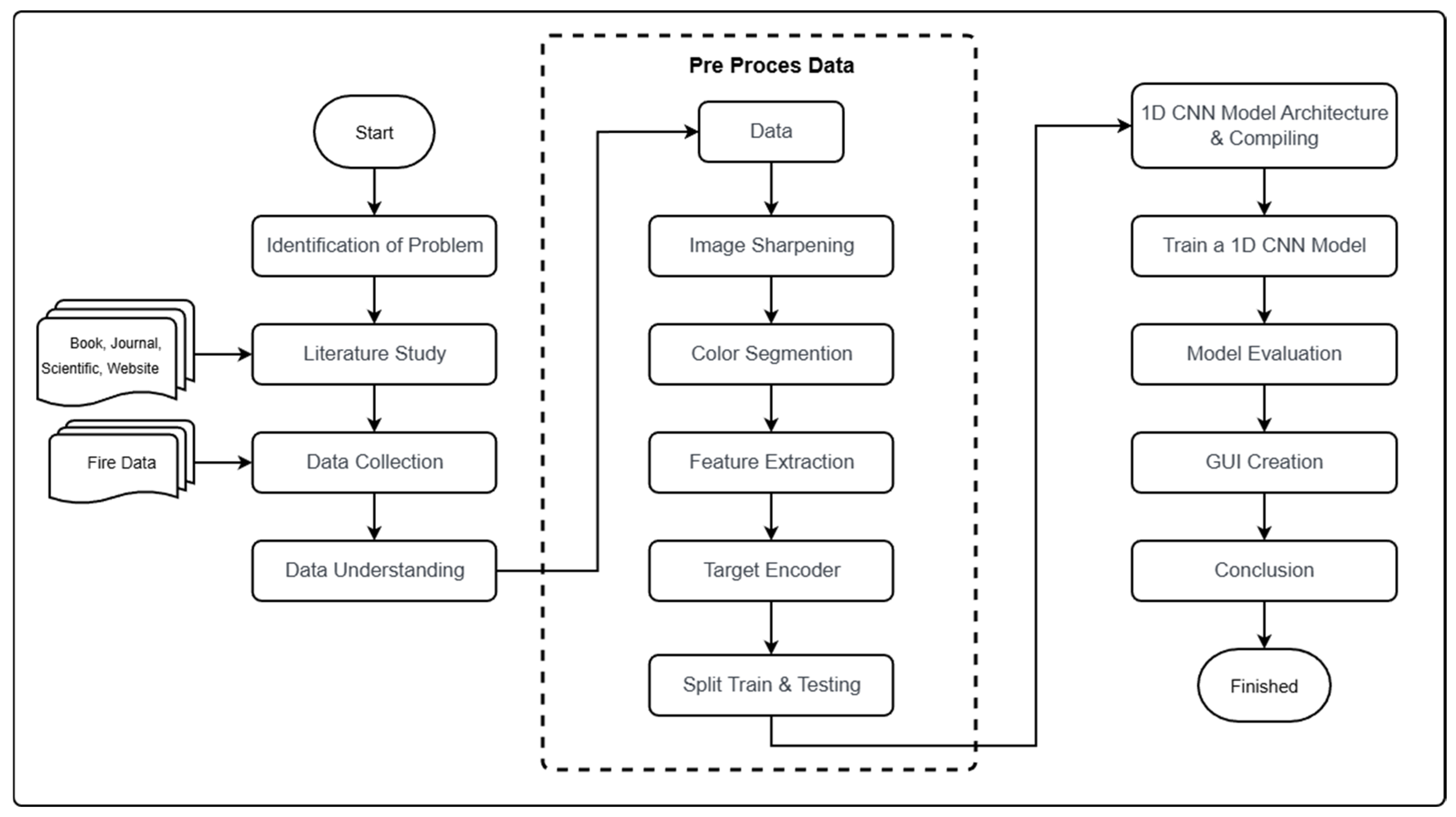
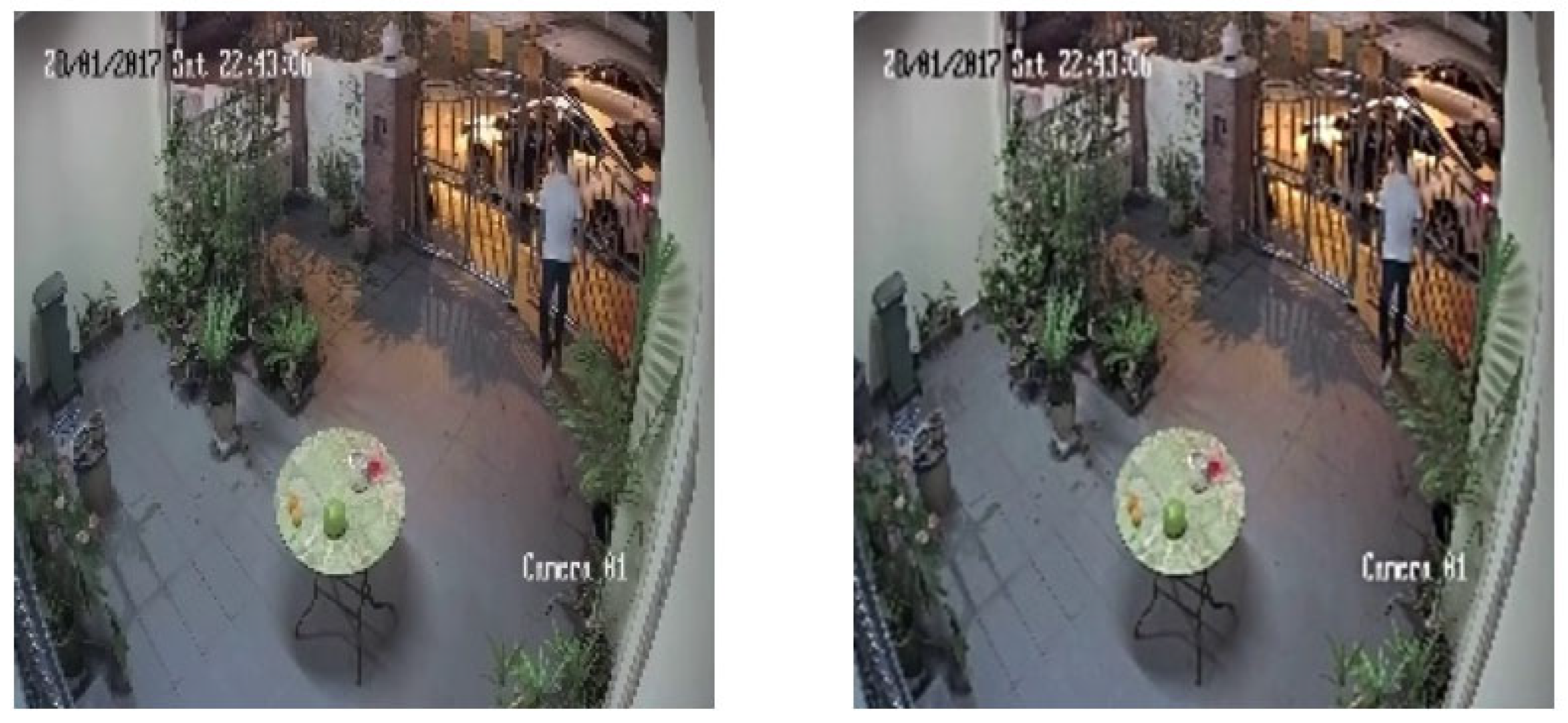
After the researcher knows a number of characteristics of the dataset that will be used, they will pre-process the data according to their observations and understanding. The data pre-processing stages that will be carried out are image sharpening, color segmentation, feature extraction, target encoder, and split train testing. Based on observations of CCTV fire images, it can be seen that the image contains noise which causes the image to become blurry. Therefore, the researchers carried out a process to increase the sharpness of CCTV images, i.e., the Gaussian Blur process was used to increase the sharpness and clarity of Figure 4.

As seen in Figure 4, there are differences in the level of image sharpness and color in various pixels, although they do not appear significant. This is because the Gaussian Blur process uses a convolution process based on the kernel size that is applied to the image after normalizing the kernel calculation itself. After the CCTV image has been observed, the image can be subjected to a color segmentation process to obtain the color values that are sought and desired from the CCTV image. In the case of fire detection, the colors that will be segmented and the values calculated are red, orange and white. This is because the fire flames are in the color range that is visible on CCTV images. So segmentation is needed for these colors in the existing image.

To carry out the color segmentation process in images, researchers can determine the lower and upper thresholds for each color that will be used in the segmentation process. The lower and upper thresholds are based on what color pixels you want to take. The RGB color arrangement for each color that will be used in the segmentation process will first be converted into HSV (Hue, Saturation, Value) color format. After determining the lower and upper thresholds, you can create a mask that searches and detects whether the color you are looking for appears in the existing CCTV image input data. The mask that will be applied to the image will be arranged based on the lower threshold and upper threshold in a predetermined HSV format. The mask that has been integrated into the image will return the capture results according to the color limitations detected in the image.

In Figure 5, it can be seen that the mask can detect previously limited colors. It can also be seen that the color areas detected by the previously created mask are dominant in orange rather than other colors. After obtaining a color area that can be detected, the next step is to carry out the process of calculating the number of colors detected based on the masking that has been performed. This number of color values will later be entered into the data frame as one of the feature parameters used in masking.

Next, the researchers pre-processed fire data based on CCTV images. It is known that CCTV images have a pixel size of 224 × 224 with three channel layers representing RGB (Red Green Blue). The researchers use the GLCM (Gray Level Co-occurrence Matrix) method for the feature extraction process; therefore, the initial stage is of course to change the CCTV image in RGB format to gray using the grayscaling process. After the CCTV image has been converted into grayscale format, the image will have the same dimensions as before with a size of 224 × 224 pixels but only one channel. After the process of converting the image to grayscale format, the next step is to carry out a binning process which divides each pixel in the image into certain binning groups. Bins are divided into several numbers, namely 0, 16, 32, 48, 64, 80, 96, 112, 128, 144, 160, 176, 192, 208, 224, 240, and 255, as shown in Figure 6

The image pixels that have been grouped into bins will be searched to determine which group appears most often in an image among these groups. The group that appears most frequently will be used as a reference level for the image. The group that appears most frequently will be searched for and its value calculated based on the pixel intensity in adjacent bins with a predetermined degree of direction reference to identify a number of features. After obtaining the value of the co-occurrence matrix based on the specified degree direction, GLCM can be used to perform statistical calculations based on various methods. These statistical calculations can be performed using contrast, homogeneity and correlation methods. With statistical calculations, it can be made easier to identify characteristics in existing images from various aspects, making it easier for learning models to understand the characteristics of image data.

Fire data based on CCTV images has target values in the form of characters. These values are default, fire, and smoke. These values must be converted into integer values because the algorithm model cannot understand the target input data in the form of characters. Therefore, it is necessary to carry out an encoder labeling process on the target data. The label encoder will change the character values in the target data into integer values based on the alphabetical order of the data. So, the default value becomes 0, fire becomes 1, and smoke becomes 2, as shown in

Table 1. Number of data test and data train.

Dataset	Kind of Data	Numbers
Fire Images From CCTV	Train Data	480
	Test Data	121

.

The final step before entering the process of creating and training an algorithm model using a 1D CNN is to divide the data into training data and test data. Fire data based on CCTV images will be divided into 80% as training data and 20% as test data. The basic reason for choosing a comparison ratio for training data of 80% and test data of 20% is the Pareto principle. In the context of dividing existing fire datasets, the Pareto principle can be applied to up to 80% of the data for training, and the evaluation results of the algorithm model can be determined with 20% of the test data. So, with 20% of the total existing data, you can determine whether the performance of the algorithm model used is good or bad.

3.4. Model 1D CNN

The results of the previous data pre-processing will be used in the model training and learning process on CCTV image data. Before carrying out the algorithm model learning process, researchers created a number of model architectures that could be used by the dataset so as to achieve the expected performance for classifying fire data based on CCTV images. The 1D CNN model architecture for fire data based on CCTV images also has three types of layers, namely convolutional layers, pooling layers, and fully connected layers. In preparing the 1D CNN architecture model for fire data based on CCTV images, it will be tested in two different architectural arrangements. Each 1D CNN model architecture for fire data based on CCTV images has two convolution layers, two pooling layers, and four connected layers.

The difference that can be seen is the addition of a dropout layer for one of the architectures. The purpose of having a dropout layer in one of the architectures is to determine the amount of performance in the algorithm model if there is a difference in the amount of network sent between existing nodes [8]. This dropout can also reduce the impact of the algorithm model experiencing overfitting. If the algorithm model experiences overfitting, then the model understands too much of the training data provided and does not understand the test data provided [9]. So, the algorithm model becomes more unstable and ineffective to use, as shown in Figure 7.

In the experimental architecture arrangement for the 1D CNN algorithm model of fire data based on existing CCTV images, both architectures have the same number of kernel sizes for input data in the first convolution layer. The quantity taken for the kernel size parameter in the first convolution layer is 5. This is because the input data that enters the algorithm model has a total of 14 features with dimensions of 1 (14, 1). So, the first layer of convolution will calculate the magnitude of the value with the weights of the 5 features simultaneously, as shown in Figure 8.

After creating the 1D CNN model architecture for fire data based on CCTV images which have been successfully compiled, we can then carry out the training process for the 1D CNN model on fire data based on CCTV images which have previously undergone feature extraction. The final dataset results that will be used are a combination of the final values of texture extraction and color extraction.

From the experimental results at epoch 500 and epoch 1000, it can be seen from the 1D CNN model architecture using dropout that the accuracy is quite good in the evaluation results. To evaluate the performance and description of the training process, further understanding is needed of the accuracy of plotting training data and test data.

As a result of plotting the accuracy of the training data and validation data in

Table 2. Trial epoch architecture with dropout.

Epoch	Accuracy Train	Recall Train	Precision Train	Accuracy Test	Recall Test	Precision Test
500	0.9083	0.9100	0.9062	0.8843	0.8843	0.8843
1000	0.9667	0.9667	0.9667	0.8512	0.8583	0.8512

it can be seen that at epoch 500, the algorithm model looks quite stable. Meanwhile, for the experiment at epoch 1000, it can be seen that the movement of the accuracy graph is quite the same as at epoch 500. However, it can be seen again at epoch 1000 that the more epoch experiments given, the more the algorithm model has the potential to experience overfitting. This can also be seen in the training results (Table 2), which show that at epoch 1000, there is a greater level of overfitting compared to the experiment at epoch 500. After determining the performance of the algorithm model using a dropout architecture, we can experiment with the algorithm with an architecture without dropout.

From the results of the accuracy of the training data and test data in

Table 3. Trial epoch architecture without dropout.

Epoch	Accuracy Train	Recall Train	Precision Train	Accuracy Test	Recall Test	Precision Test
500	0.9375	0.9375	0.9395	0.9008	0.9000	0.8926
1000	0.9771	0.9771	0.9771	0.9090	0.9090	0.9090

, it is known that the resulting accuracy is better than the 1D CNN architecture that uses dropout. However, it can also be seen that the results of accuracy, precision and recall on training data and test data have quite visible differences and exceed the differences of the 1D CNN architecture using dropout. So, from Table 3, it can be concluded that the 1D CNN algorithm model also experiences overfitting.

As seen in the plotting in Table 3, the accuracy pattern results given at epoch 500 and epoch 1000 with the architecture without dropout are similar to those of epoch 500 and epoch 1000 with the architecture using dropout. Each architecture is still able to increase accuracy at epoch 500 and become stable at epoch 1000 in experiments. However, the difference that can be seen between Table 2 and Table 3 is the level of overfitting. Architectures that do not use dropouts tend to have greater overfitting values compared to architectures that use dropouts, which can be seen visually in the existing plotting images. A comparison of the amount of overfitting can be seen in

Table 4. Comparison of overfitting values based on accuracy.

Architecture	Epoch	Train Data Accuracy	Test Data Accuracy	Overfitting Value
Dropout	500	0.9083	0.8843	0.0240
	1000	0.9667	0.8512	0.1155
Without Dropout	500	0.9375	0.9008	0.0367
	1000	0.9771	0.9090	0.0681

.

After knowing the accuracy performance and level of overfitting in each 1D CNN model architecture, which can be seen from Table 4 along with graphic images in Figure 8, the researcher will use the 1D CNN architecture using dropout to reduce the level of overfitting in the algorithm model. Even though researchers use dropout layers to reduce the level of overfitting in the 1D CNN algorithm model, a level of overfitting still exists in the algorithm model even though the value is below 3%. Therefore, the researchers carried out another experiment, namely by adding the kernel_regularizer parameter in one of the layers, which aims to reduce the weight value of each learning algorithm model per epoch.

It can be seen that based on the accuracy, precision and recall values in

Table 5. Trial epochs with kernel regularizer.

Epoch	Accuracy Train	Recall Train	Precision Train	Accuracy Test	Recall Test	Precision Test
500	0.7729	0.7604	0.7749	0.7273	0.7190	0.7311
1000	0.8667	0.8625	0.8679	0.8099	0.8099	0.8167

regarding the use of kernel regularizer parameters, the metric values produced in both epochs look smaller than without using kernel regularizer parameters. This is due to the use of lower weight values for the learning or training input data. This is in accordance with the aim of using the kernel regularizer itself, namely to reduce or suppress the level of overfitting that exists in the 1D CNN algorithm model [10]. This can also be observed from the existing graph, which shows clearer comparisons of architectures that use kernel regularizers and those that do not use kernel regularizers.

Based on Table 5 which contains the plotting of the algorithm model training results, it can be seen that the distance between the training data and the experimental validation data is not as far as with a dropout architecture that does not use a kernel regularizer. It can be seen that using the kernel_regularizer parameter in the layer can further reduce the level of overfitting in this one-dimensional CNN algorithm model. The results of the test data metrics for the dropout architectural model that uses a kernel regularizer and one that does not use a kernel regularizer can be seen in

Table 6. Results with and without kernel regularizer.

Epoch	Accuracy with Kernel Reg	Recall with Kernel Reg	Precision with Kernel Reg	Accuracy Without	Recall Without	Precision Without
500	0.7273	0.7190	0.7311	0.8843	0.8843	0.8843
1000	0.8099	0.8099	0.8167	0.8512	0.8583	0.8512

below.

However, when compared with the dropout architecture without using regularizer kernel parameters, it can be seen in Table 6 above that the architecture that uses dropout without regularizer kernel parameters is a better option at epoch 500 in terms of the metric value. So, we will use a dropout architecture without a kernel regularizer in 500-epoch experiments for the classification and detection of existing input data.

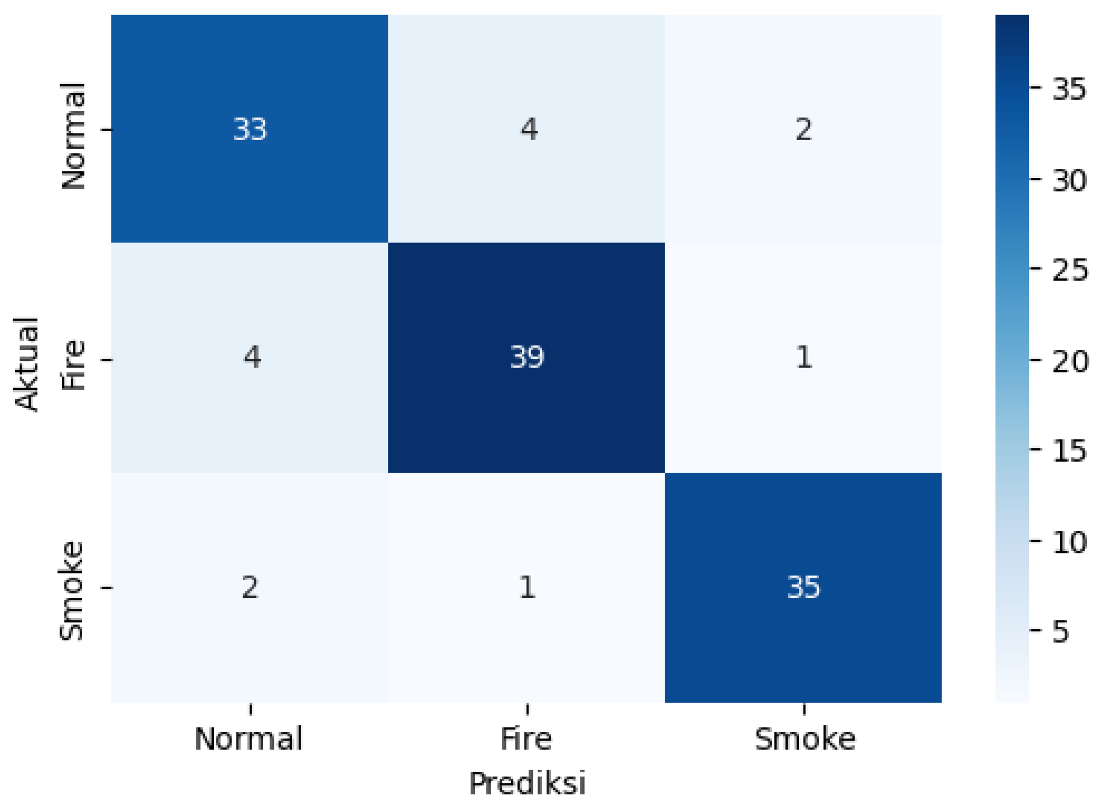
As seen in the confusion matrix (Figure 9), based on the existing training data and test data, the algorithm model can perform normal, fire and smoke detection well. A total of 107 data points were detected correctly, including 33 for normal, 39 for fire, and 35 for smoke. So, if the percentages are calculated, 84% of the normal data is detected correctly, 88% of the fire data is detected correctly, and 92% of the smoke data is detected correctly. Next, the researchers conducted fire input data experiments based on CCTV images separate from the previously determined training data and test data. This detection experiment used three images captured by CCTV—a fire CCTV image, a non-fire CCTV image and a smoky CCTV image—which were entered into the algorithm model manually.

The CCTV image input data that has been prepared has different dimensions. Therefore, in this experiment with CCTV image input data, the image dimensions will be resized to 224 × 224 pixels. After entering fire CCTV image data, the 1D CNN algorithm model is expected to be able to detect that the CCTV image is a fire image, so it returns the output “Fire!”. Meanwhile, for CCTV image input data that does not have a fire, it is hoped that it will be able to successfully detect that there is no fire in the image and return the output “Normal”. For smoky CCTV image input data, the algorithm model is expected to be able to carry out appropriate detection by returning the output “Smoke!”.

Based on the detection results using input images separate from the training data and test data in

Table 7. Result detection with manual input.

Category	Numbers	Detection Result
Fire	5	2 Fire, 2 Smoke, 1 Normal
Normal	3	1 Fire, 2 Smoke, 0 Normal
Smoke	3	1 Fire, 0 Smoke, 2 Normal

above, it can be seen that there are input images that were not detected correctly. This happens because in the process of changing the input image from dimension 2 to dimension 1, it has a number of texture value patterns or levels of color which have output results between the range of values understood by the algorithm model for certain types of classes. So, the algorithm model considers the input data to be what was studied previously and requires more complex two-dimensional to one-dimensional image data processing than texture feature extraction and color segmentation.

3.5. Result of GUI Development

After carrying out the modeling process using a 1D CNN for fire data based on CCTV images, the researchers created an interface that was easy to understand. However, before carrying out the GUI creation process further, the 1D CNN algorithm model for fire data based on CCTV images will be exported into h5 format so that the model can be used in the GUI. The interface itself was created using the default Python (Version 3.10.8, Python Software Foundation) library, namely Tkinter. The main window has two selection buttons according to our needs and uses. The first is a button to detect fires based on manual image input media, and the second button is an option to input image data in real time, as shown in Figure 10.

The next step is to create an access display to input data into the algorithm model in the two existing GUI button options. On the button that says “Browse Images from Library”, the action expected from the GUI is to select an image file. On the button with this action, the user can manually select fire image data from CCTV and it will immediately detect whether there is a fire or not from the CCTV image entered, as shown in Figure 11.

If the user chooses to experiment with input data using the “Open Camera Live Detection” button, the input data will be entered into the algorithm model in real time and an output will immediately be returned based on the detection results of the algorithm model. This real-time detection uses an external camera device which is assumed to be a CCTV camera.

4. Conclusions

In this research, an algorithm model system has been prepared and designed using 1D CNN (One-Dimensional Convolutional Neural Network) to carry out the fire detection process based on existing CCTV image datasets. So, it is known that the performance of the algorithm model using the One-Dimensional Convolutional Neural Network method produces accuracy, recall and precision metrics of 88.43% on test data with an architecture that uses dropout layers with epochs of 500. In addition, it is known that the algorithm model can run on a GUI-based application using the built-in library of the Python programming language and produces detection results using real data when real-time detection and manual input are not good enough because the One-Dimensional Convolutional Neural Network algorithm accepts values in a range known to the model. So, we need additional related image processing processes that can identify the characteristics of existing image data before the detection process is carried out.

The advice that the researchers can give to future researchers if they want to use the same themes and topics is to process image data further, rather than limiting themselves to the GLCM process or image masking to obtain certain values that represent the image entered into the data frame to carry out evaluations. The results of image color segmentation allow users to appropriately retrieve a desired object in the image based on color. Apart from that, the researchers suggest that future researchers use a two-dimensional convolutional neural network algorithm to carry out detection or classification if the data used comes from image data, and use supporting elements such as sensors to support the decision on whether there is a fire or not.