Abstract
This study analyzes air pollution time-series big data to assess stationarity, seasonal patterns, and the performance of machine learning models in forecasting PM2.5 concentrations. Fifty-two low-cost sensors (LCS) were deployed across Krakow city and its surroundings (Poland), collecting hourly air quality data and generating nearly 20,000 observations per month. The network captured both spatial and temporal variability. The Kwiatkowski–Phillips–Schmidt–Shin (KPSS) test confirmed trend-based non-stationarity, which was addressed through differencing, revealing distinct daily and 12 h cycles linked to traffic and temperature variations. Additive seasonal decomposition exhibited time-inconsistent residuals, leading to the adoption of multiplicative decomposition, which better captured pollution outliers associated with agricultural burning. Machine learning models—Ridge Regression, XGBoost, and LSTM (Long Short-Term Memory) neural networks—were evaluated under high spatial and temporal variability (winter) and low variability (summer) conditions. Ridge Regression showed the best performance, achieving the highest (0.97 in winter, 0.93 in summer) and the lowest mean squared errors. XGBoost showed strong predictive capabilities but tended to overestimate moderate pollution events, while LSTM systematically underestimated PM2.5 levels in December. The residual analysis confirmed that Ridge Regression provided the most stable predictions, capturing extreme pollution episodes effectively, whereas XGBoost exhibited larger outliers. The study proved the potential of low-cost sensor networks and machine learning in urban air quality forecasting focused on rare smog episodes (RSEs).
1. Introduction
The impact of air pollution on human health is profound with particulate matter (PM) being a major contributor to various medical conditions. PM consists of various particles with a diameter of 10 microns and less—PM10, a diameter of 2.5 microns and less—PM2.5, a diameter of 1 microns and less—PM1. Such small particles can be inhaled and later be transported with blood. Studies indicate that exposure to PM contributes to a notable percentage of global illnesses and fatalities [1]. Its effects extend much beyond typical respiratory issues [2] including lung cancer [3], coronary diseases [4], and even low birth weight and pregnancy complications [5]. What is more, research also links it to neurological disorders like Parkinson’s and Alzheimer’s [6]. This poses significant challenges for countries with aging populations, where healthcare demands are already high. It is clear that air pollution including PM is a critical global challenge with both immediate and long-term consequences for public health. Beyond human health, air pollution severely disrupts natural ecosystems. It negatively impacts biodiversity, damages forests, contaminates water supplies and reduces agricultural productivity, further destabilizing the environment [7].
It is clear that prolonged exposure to particulate matter (PM) significantly contributes to respiratory and cardiovascular diseases as well as increased mortality rates. Observations conducted in Thailand reveal a strong correlation between PM pollution and mortality with smog episodes predominantly occurring during the dry season [8]. A comparable situation is observed in Brazil, where residual heating—one of the primary contributing factors—is closely linked to elevated PM concentrations [9]. In Poland, smog episodes are primarily a winter phenomenon. During the summer, PM pollution remains at relatively low levels, except for occasional spikes caused by events such as agricultural burning, which can temporarily increase pollutant concentrations [10,11].
Krakow serves as an excellent case study for air quality research due to its stringent air pollution control measures, including a complete ban on solid fuel usage for household heating. Despite these regulations, the city continues to experience severe smog episodes during late autumn, winter, and early spring, particularly when temperatures drop below 0 °C [12]. During these periods, Krakow frequently ranks among the most polluted cities in the world. This persistent issue is largely attributed to the city’s geographic positioning in a valley, which creates unfavorable dispersion conditions, as well as specific meteorological factors that trap pollutants near the surface. Additionally, pollution from neighboring municipalities, where solid fuel combustion remains widespread, is transported into Krakow via atmospheric migration and diffusion, exacerbating local air quality degradation [13]. In response, municipal authorities actively monitor smog conditions, providing real-time public alerts and implementing emergency measures such as free public transportation and advisories against outdoor physical activity during high-pollution episodes. It is worth understanding the research area at the regional scale. The Malopolska region’s strategy outlines the geographical conditions [14], while the terrain and near-surface geological features are detailed in [15,16].
Accurate smog event prediction is crucial for effective air quality management. This study uses data from 52 LCS based on light-scattering technology to evaluate various forecasting models, including Ridge Regression [17], XGBoost [18], and Long Short-Term Memory (LSTM) networks [19]. This study utilizes data from 52 LCS based on light-scattering technology to analyze time-series data and evaluate the performance of various forecasting models. Seasonal decomposition was applied to capture the seasonal, residual, and trend components to study periodic patterns. Autocorrelation (ACF) and partial autocorrelation (PACF) plots were also used to assess time-dependencies in the data. Instead of focusing solely on traditional methods, this study explores machine learning models, including Ridge Regression, XGBoost, and Long Short-Term Memory (LSTM) networks, to assess their effectiveness in predicting PM2.5 concentrations and rare smog episodes (RSEs). A key aspect of the analysis was residual analysis, which revealed the performance of the models, particularly during high-variability smog events in December. While the LCS used in this study are less precise than reference-grade monitoring stations that use gravimetric techniques, previous studies have shown a strong correlation between LCS readings and reference data [12], validating their reliability for air quality monitoring. By leveraging both traditional statistical methods and machine learning models, this study aims to enhance the forecasting capabilities for air quality, ultimately contributing to better air quality management strategies and more informed public health decision making.
2. Materials and Methods
2.1. Data Analysis
An analysis was conducted on a measurement dataset comprising data from 52 Airly LCS (www.airly.com) located in the Krakow area. Each sensor records PM1, PM2.5, and PM10 concentrations and meteorological parameters like temperature, relative humidity, or surface pressure with 1 h time resolution. The data were collected throughout the year 2022. Almost all time-series analysis methods assume the stationarity of time series (including autocorrelation), which means that its statistical properties, such as mean and variance, remain constant over time. If a time series is non-stationary, it can lead to incorrect conclusions in statistical analysis [20]. The KPSS test (Kwiatkowski–Phillips–Schmidt–Shin) showed that the PM2.5 time series is non-stationary with respect to the trend [21]. Therefore, before proceeding with ACF and PCAF analysis, first-order differencing was applied. ACF and PACF analyses were conducted according to Equation (1):
where the following apply:
- —the change in the observation value between time t and ,
- —the observation value at time t,
- —the observation value at time .
After the ACF analysis, the PM2.5 series was effectively decomposed. Both additive and multiplicative seasonal decomposition (for time-inconsistent noise) techniques were applied to analyze the series components [22]. A time series consists of three main components representing the seasonal factor, trend, and residual part [23]. For an additive time series, the overall observation is expressed as the sum of its components, as represented in Equation (2).
where the following apply:
- —the time series,
- —seasonality in the time series,
- —trend in the time series,
- —residual values in the time series.
In the case of a multiplicative time series, the series is modeled as the product of its components. Applying a logarithmic transformation converts this model into an additive form by transforming the multiplicative relationships into additive ones. This transformed series can then be expressed as the sum of the logarithms of the individual components, as shown in Equation (3).
2.2. Data Workflow
Following the initial data analysis, a robust processing pipeline was developed using the Kedro framework [24]. This pipeline automatically generated 14 additional covariates for PM2.5, applied data scaling, and imputed missing values through linear interpolation while optimizing memory usage via the downcasting of data types. Lagged features were created using the Darts library, ensuring the prevention of data leakage [25]. The entire workflow was integrated with the GitLab platform (www.gitlab.com) and a continuous integration/continuous deployment (CI/CD) pipeline.
2.3. PM2.5 Concentrations Forecasting
In this study, three machine learning models were applied to forecast PM2.5 concentrations:
- LSTM (Long Short-Term Memory) is a type of recurrent neural network (RNN) designed to process sequential data by maintaining long-term dependencies. In the context of time-series forecasting, LSTMs learn patterns from past observations and use their memory cells to retain relevant information, allowing them to predict future values more accurately while mitigating issues like vanishing gradients [19].
- XGBoost (Extreme Gradient Boosting) is an optimized gradient boosting framework that enhances predictive performance through regularization, parallel processing, and efficiently handling missing data. In time-series forecasting, XGBoost constructs an ensemble of decision trees by iteratively minimizing the residual errors, effectively capturing complex temporal dependencies and nonlinear relationships in the data [18]. XGBoost proved strong performance in spatiotemporal tasks and consistency with prior studies [26], though LightGBM is also a strong alternative [27].
- Ridge Regression is a linear regression technique that incorporates an regularization term to prevent overfitting by penalizing large coefficient magnitudes. In time-series forecasting, Ridge Regression helps model temporal dependencies by maintaining stability in parameter estimates especially when dealing with multicollinearity or highly correlated lagged features [17].
The performance of each model was rigorously validated using a backtesting procedure, ensuring that predictions were made solely based on data available before the forecast date. Two distinct periods were analyzed: the summer period, characterized by low spatial and temporal variability in PM2.5 concentrations, and the December period, which captured the higher variability typically observed during the autumn–winter season.
The performance of LSTM, XGBoost, and Ridge Regression models was evaluated using standard error metrics. Mean Absolute Percentage Error (MAPE) is a scale-independent measure that quantifies the average percentage deviation of predictions from actual values. Mean Absolute Error (MAE) represents the average absolute difference between predicted and observed values. Mean Squared Error (MSE) penalizes larger errors more heavily by averaging the squared differences between predicted and actual values. The coefficient of determination (R2) indicates the proportion of variance in the dependent variable explained by the model. The box plots were used to analyze the distribution of residuals (differences between the actual and predicted values) for the Ridge and XGBoost models in December. A box plot is a statistical visualization tool that represents the spread and variability of a dataset by displaying the median, quartiles, and potential outliers. It provides a concise summary of the residual distribution, allowing for a visual inspection of model performance. By examining the residual box plots, patterns such as skewness, dispersion, and the presence of outliers can be identified, offering insights into the accuracy and consistency of each model.
3. Results
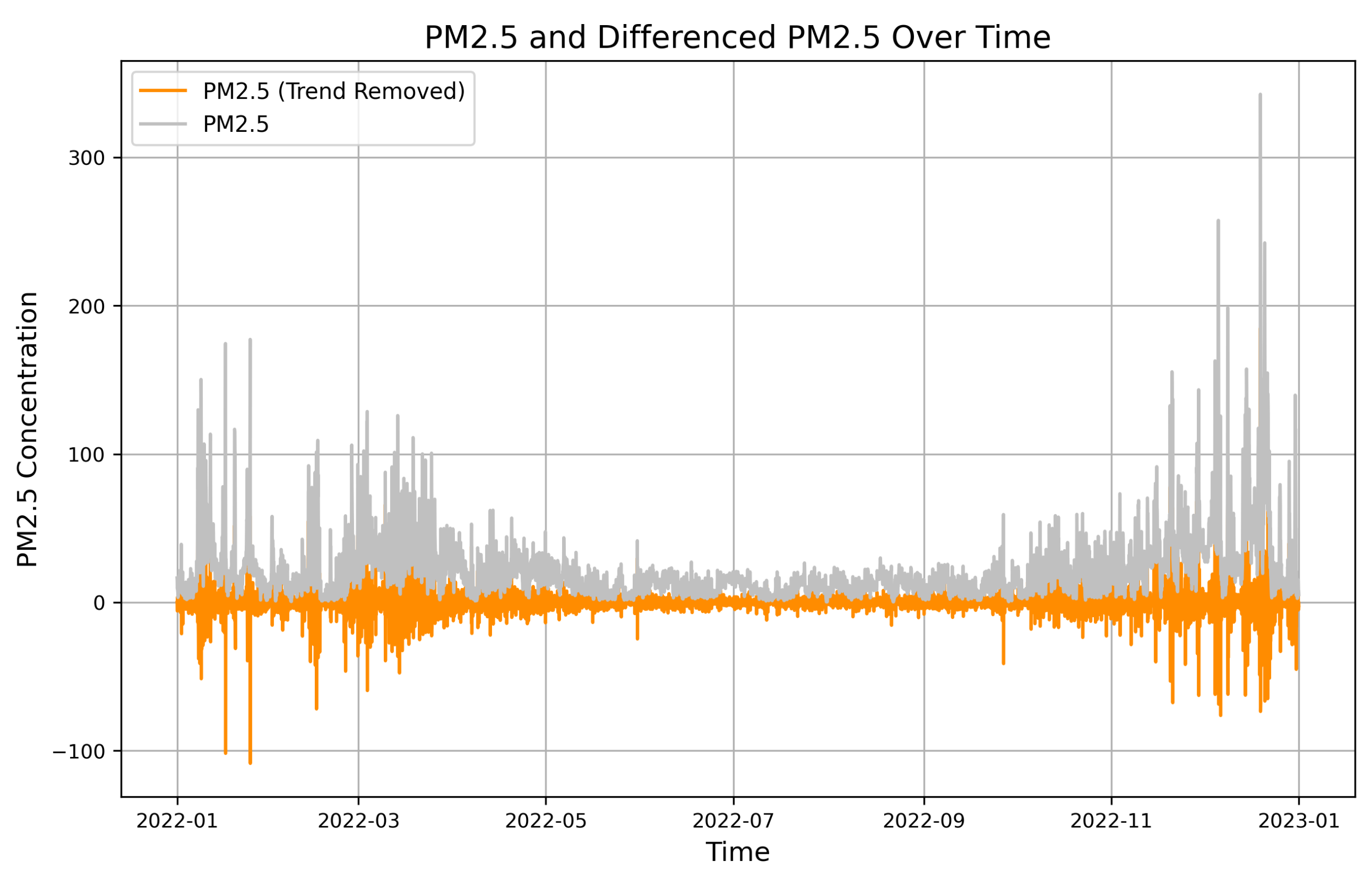
The KPSS test indicated that the PM2.5 time series is non-stationary with respect to the trend [21]. The results of differentiation transformation are shown in Figure 1.

Figure 1.
Differenced PM2.5 Time Series to Address Non-Stationarity.
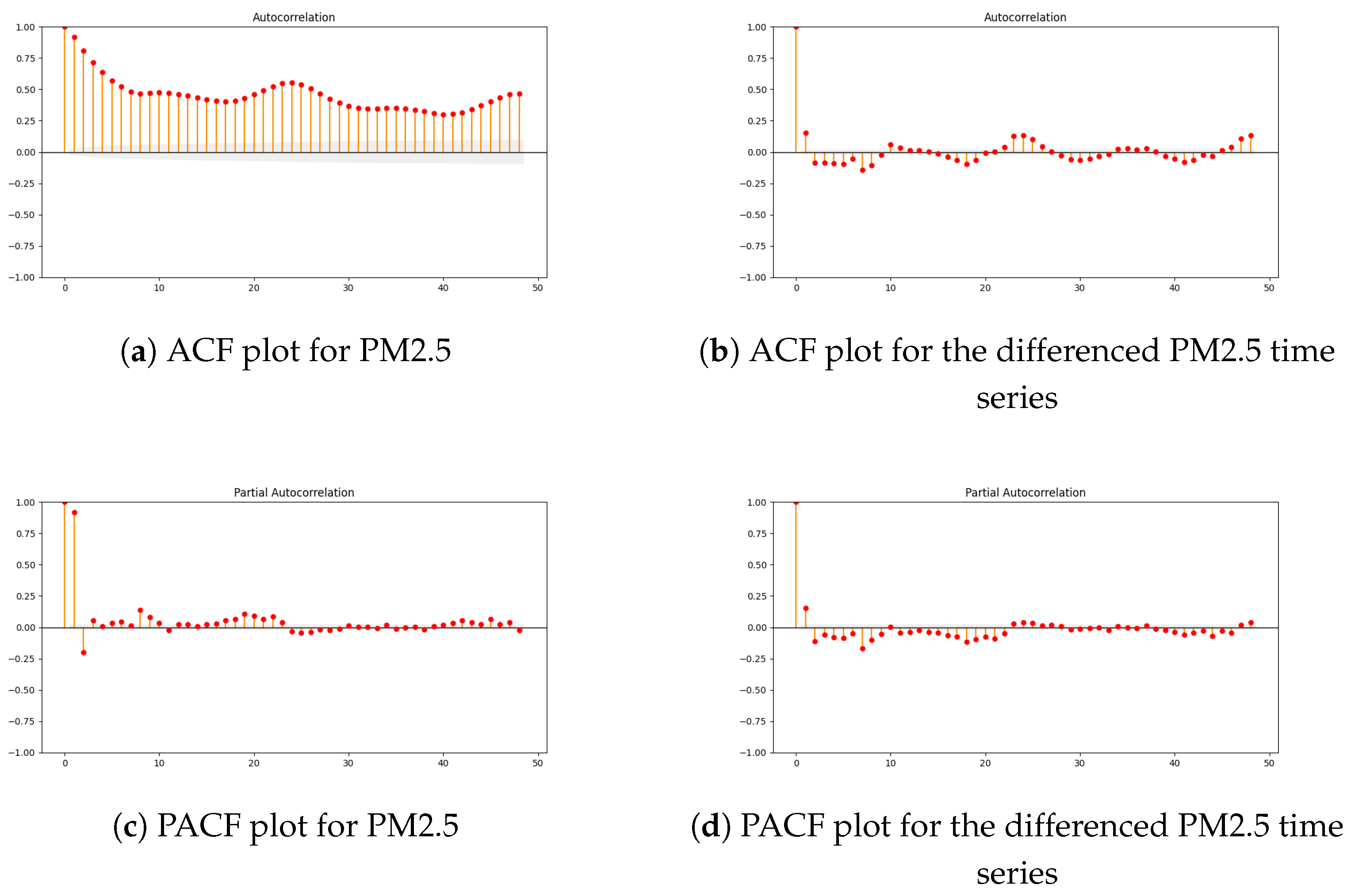
The results indicate that after the transformation, PM2.5 values started fluctuating around zero. This transformation effectively removed non-stationarity concerning the trend and clarified the ACF. However, the differencing operation did not have a significant impact on the PACF. The autocorrelation plots show clear daily cycles (Figure 2) as well as smaller 12 h seasonal patterns likely linked to peak traffic times and solar movement. The daily temperature cycle, driven by similar morning and evening temperatures, follows a sinusoidal pattern, which becomes distinctly visible in the ACF plot after differencing.

Figure 2.
Autocorrelation Function (ACF) and Partial Autocorrelation Function (PACF) plots for PM2.5 and its differenced time series.
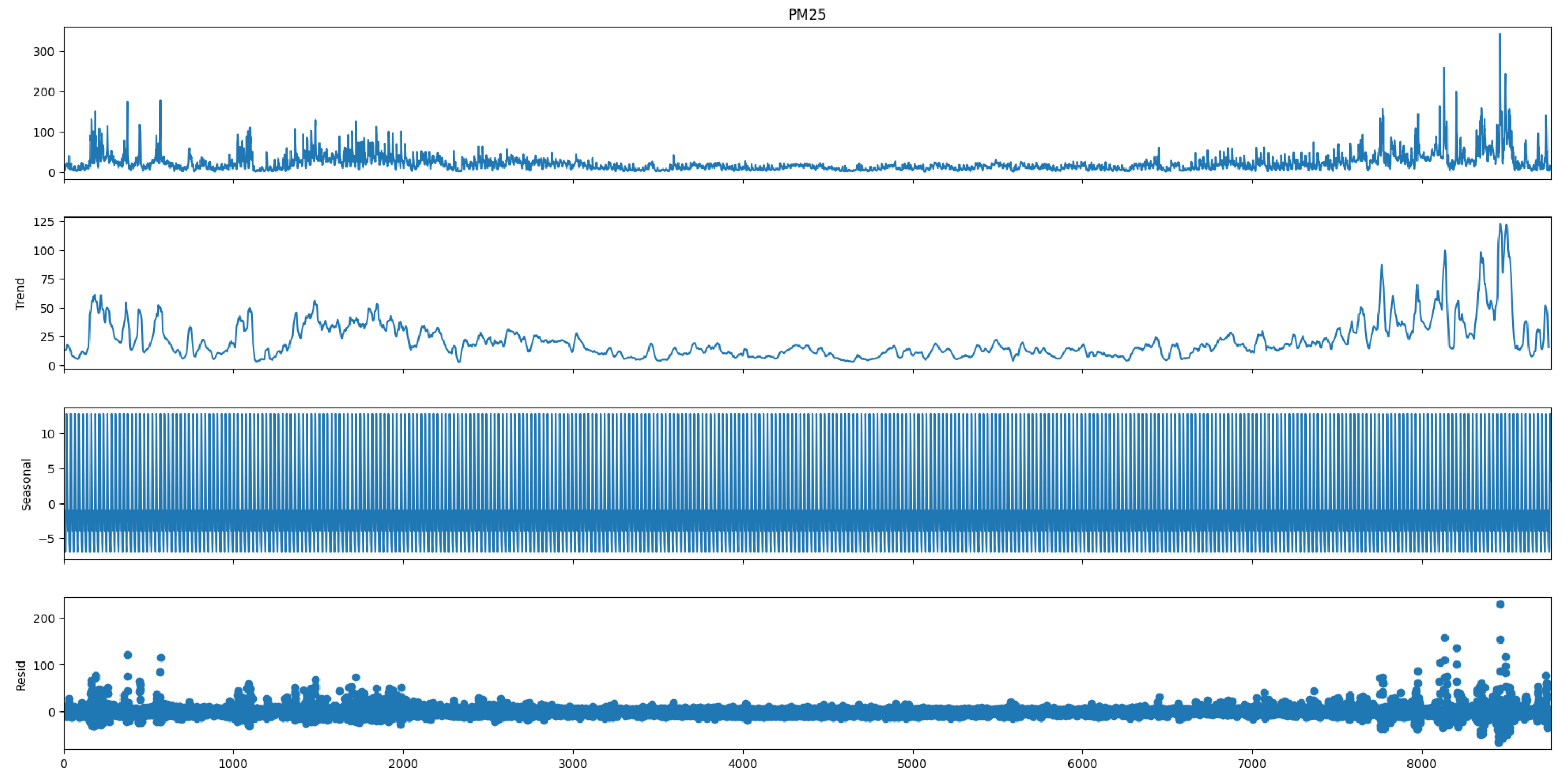
Figure 3 shows additive seasonal decomposition results. The residual values are inconsistent over time (the average level of oscillations in the middle of the time series differs from those at both ends). Between hours 2000 and 6500, the noise appears flatter compared to the series ends, indicating that the variance changes over time. This suggests that it is not typical white noise. This observation implies that the additive decomposition did not fully capture some aspects of the decomposition process. Additionally, a visible trend and seasonality can be observed.
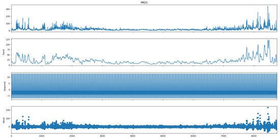
Figure 3.
Additive Seasonal Decomposition of PM2.5 Time Series for the whole year.
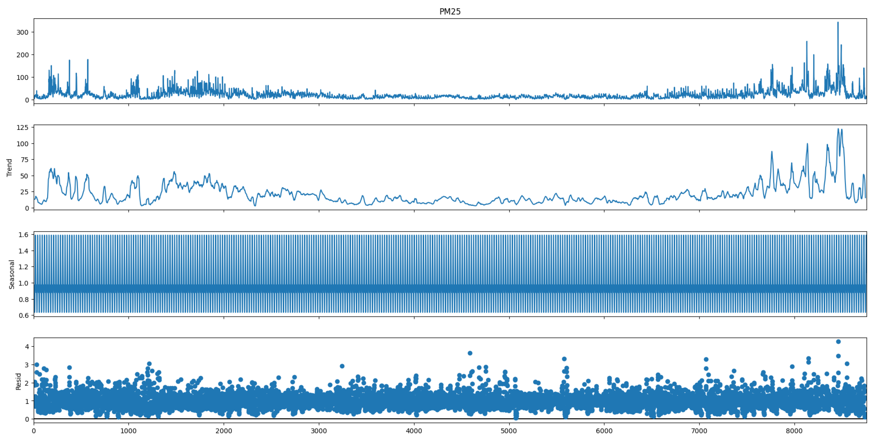
To address the issue of time-inconsistent noise, a multiplicative decomposition was performed [28]. After applying this method, noticeable changes in the residual values were observed. Following the multiplicative decomposition (Figure 4), due to the logarithmic transformation, the residual values began oscillating around 1 µg/m3, and outliers emerged during the summer months. These outliers are most likely caused by grass burning in surrounding agricultural fields, which results in wind-driven pollution transport, leading to increased PM2.5 concentrations around the sensors.
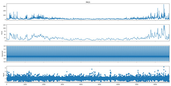
Figure 4.
Multiplicative Seasonal Decomposition of PM2.5 Time Series for the whole year.
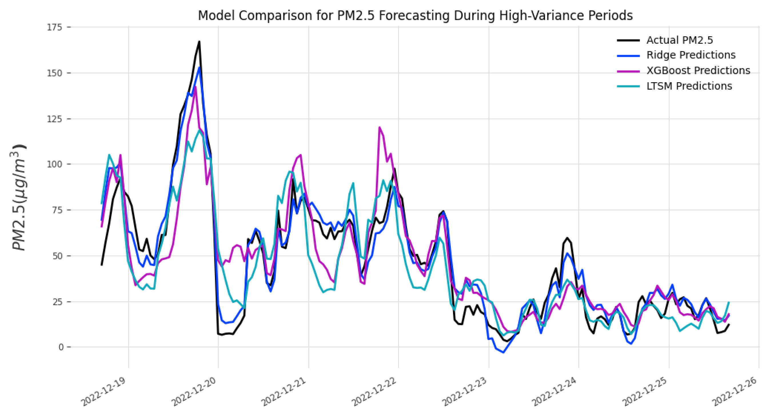
Figure 5 shows the PM2.5 prediction results for December, a month characterized by high spatial and temporal variability in pollution levels. Significant peaks are clearly visible, reaching 175 µg/m3, which considerably exceeds the allowable limits. The best fit for the majority of RSE was obtained using the Ridge Regression model. Table 1 presents the error metrics. The R2 for Ridge Winter is as high as 0.97, with a MSE of only 14.88. Both LSTM and XGBoost performed worse. In the case of moderate peaks, the XGBoost model tended to overestimate the values (12/21/2022 and 12/22/2022), whereas it performed better for extreme episodes (12/20/2024). XGBoost was characterized by a high MSE of over 46 (µg/m3)2 but still maintained a relatively good R2 of 0.87. The LSTM model, on the other hand, consistently tended to underestimate the values with R2 of 0.81.

Figure 5.
PM2.5 Prediction Results for December—High Temporal and Spatial Variability: Real Observation (black); Ridge Regression Predictions (dark blue); XGBoost Predictions (purple); LSTM Predictions (light blue).

Table 1.
Performance Metrics for Ridge, XGBoost, and LSTM Models during Winter and Summer Seasons. The table presents key error metrics (MAPE, MAE, MSE, and R2) for Ridge Regression, XGBoost, and LSTM models in both seasons.
Figure 6 shows the PM2.5 prediction results for July, a month characterized by low spatial and temporal variability in pollution levels. There are no significant peaks and concentrations are within the notm with maximim value 12 µg/m3, which is almost 15 times lower than in December. Again the best results were obtained using the Ridge Regression model and the worst with LSTM. The R2 for Ridge in Summer is 0.93, with a MAE of only 1 (µg/m3) which is below the sensor accuracy. The XGBoost model showed very similar results to Rdige with R2 0.92 and MAE 1.18 (µg/m3). The LSTM model, on the other hand, consistently tended to give the less accurate prediction with R2 of only 0.57.
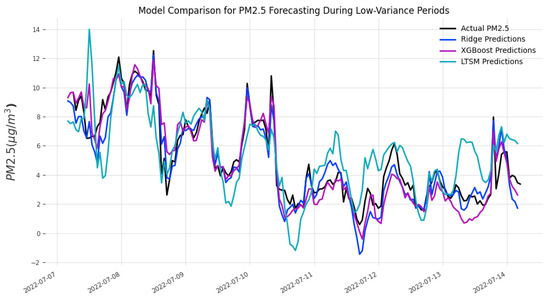
Figure 6.
PM2.5 Prediction Results for July—Low Temporal and Spatial Variability: Real Observation (black); Ridge Regression Predictions (dark blue); XGBoost Predictions (purple); LSTM Predictions (light blue).
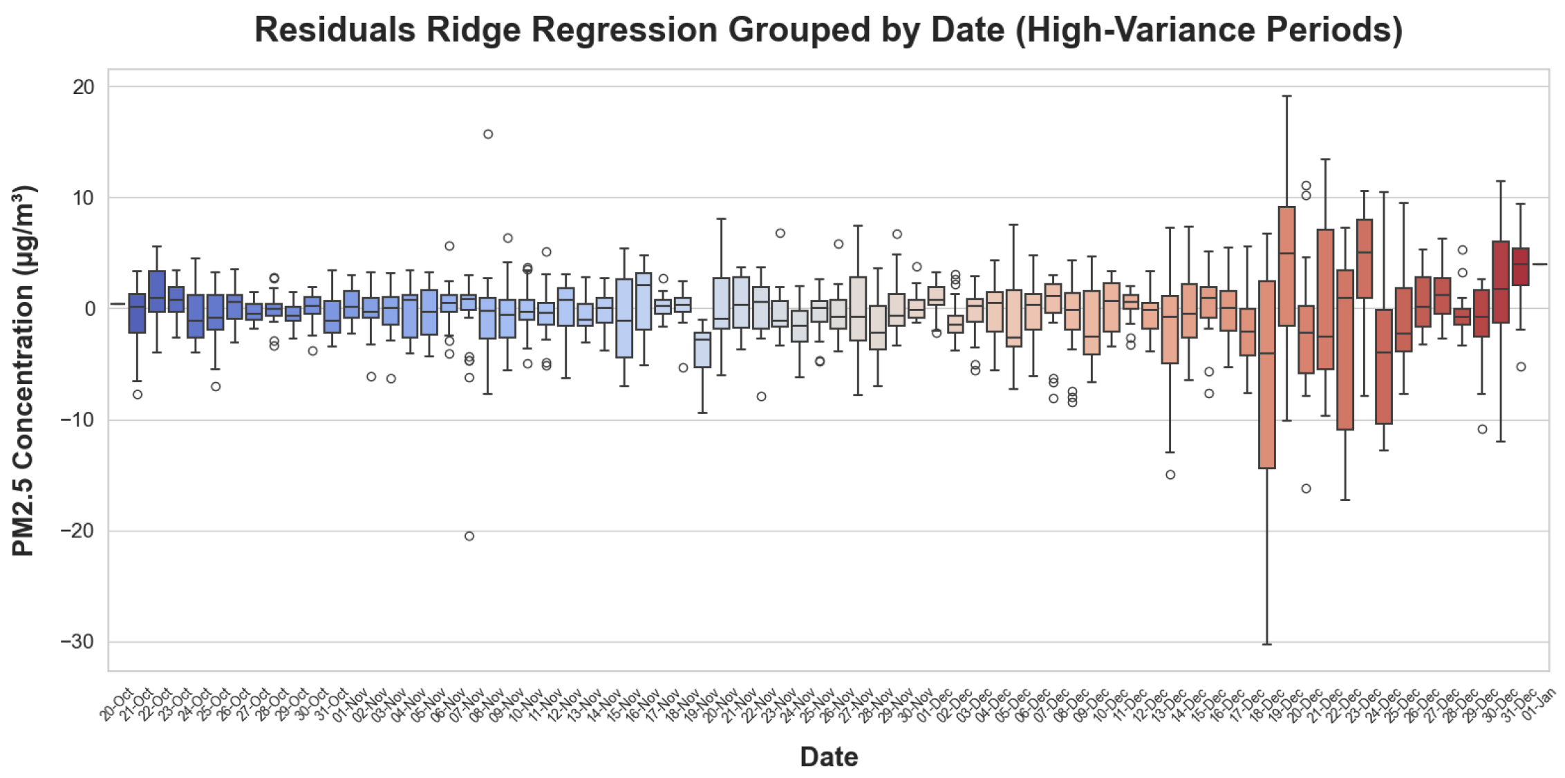
Box plots were used to compare the residuals for each day of the month with the highest variability (December) between the two top-performing models, Ridge and XGBoost. In the autumn-winter season, characterized by substantial fluctuations in PM2.5 levels with significant smog episodes, XGBoost typically maintains a central cluster of residuals around the median but occasionally produces large outliers, with values reaching up to ±40 µg/m3 (Figure 7). Ridge Regression also had significant deviations in some days but seems to handle the most extreme fluctuations more effectively, typically containing the majority of residuals within a narrower, more consistent range with a maximum ±20 µg/m3 (Figure 8).
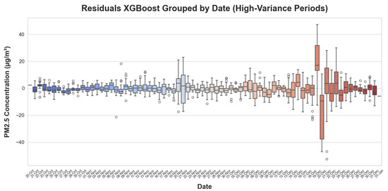
Figure 7.
Box Plot of PM2.5 Residuals for December: XGboost Model Performance.
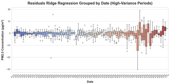
Figure 8.
Box Plot of PM2.5 Residuals for December: Ridge Model Performance.
4. Discussion
The results of this study provide valuable insights into the spatiotemporal characteristics of PM2.5 pollution with a focus on the machine-learning forecasting of RSE. The particular focus was Krakow and its surroundings; however, the results of this study can have wider applicability in similar areas within moderate climate zones. The use of 52 LCS allowed for high-resolution spatial and temporal analysis with hourly measurements generating nearly 40,000 observations over the two-month study period. This extensive dataset provided a detailed representation of pollution patterns, demonstrating strong seasonal and diurnal variability.
The KPSS test confirmed that the PM2.5 time series exhibited trend-based non-stationarity. Differencing allowed removing the trend component, showing clear daily and 12 h periodic patterns which are primarily driven by urban traffic emissions and temperature variations within the day–night frame. The autocorrelation analysis further reinforced these patterns, highlighting the clear seasonality of PM2.5 levels. This is an important observation proving that the forecasting of PM2.5 levels should include long and short-term seasonality. The additive decomposition method struggled with time-inconsistent residuals. Therefore, PM2.5 variability could not be fully captured by a linear seasonal-trend model. The multiplicative decomposition provided a more stable residual component, though it introduced visible outliers during summer, which was most likely due to episodic pollution events such as agricultural burning. This suggests that seasonal decomposition alone may not fully capture external influences on PM2.5 concentrations and that additional environmental factors should be considered in future studies.
During winter, PM2.5 levels showed significant fluctuations, with frequent RSEs exceeding 175 µg/m3, far beyond air quality standards. December RSEs are related mostly to residual heating [26]. In contrast, summer months exhibited low spatial and temporal variability, with PM2.5 concentrations remaining below 12 µg/m3, which is nearly 15 times lower than winter levels. The absence of major pollution peaks in summer suggests that secondary sources, such as transport and manufacturing emissions, play a significantly smaller role compared to winter residual heating.
The forecasting experiments highlighted the varying effectiveness of Ridge Regression, XGBoost, and LSTM models under different seasonal conditions. Ridge Regression consistently outperformed other models, achieving the highest R2 values (0.97 in winter, 0.93 in summer) and lowest error metrics. The model’s performance suggests that this approach effectively captures the underlying trends and seasonal cycles in PM2.5 data. Ridge Regression showed more stable residual distributions in December, proving its robustness against RSE. XGBoost, a tree-based ensemble model, performed well in most cases but exhibited overestimation during moderate pollution events and underestimation during extreme pollution episodes. While it captured the general trends, its performance was less stable and produced higher outliers than Ridge Regression in RSE. The LSTM model performed the worst among the three with a noticeable underestimation of PM2.5 concentrations. This was particularly evident during winter, where its R2 dropped to 0.81, indicating difficulty in capturing the sudden and extreme pollution peaks. The lower accuracy suggests that despite LSTM’s ability to model temporal dependencies, it may require additional hyperparameter tuning, feature engineering or larger datasets for more reliable predictions.
The study confirms that PM2.5 pollution in Krakow exhibits strong seasonal dependence. The effectiveness of Ridge Regression suggests that linear models, when appropriately tuned, can offer highly accurate PM2.5 predictions. However, the limitations of XGBoost and LSTM indicate the need for further research into hybrid models that combine the strengths of multiple approaches.
Future work should explore deep learning architectures for enhanced time-series forecasting and integrate geostatistical methods to account for spatial dependencies. Another crucial aspect is to use Explainable AI (XAI) to evaluate real-time PM2.5 forecasting models for air quality monitoring and public health decision making.
Author Contributions
Conceptualization, M.Z.; methodology, M.Z. and S.C.; validation, M.Z., S.C. and T.D.; formal analysis, M.Z. and S.C.; investigation, M.Z. and S.C.; resources, M.Z. and S.C.; data curation, T.D.; writing—original draft preparation, M.Z. and S.C.; writing—review and editing, M.Z. and S.C.; visualization, M.Z. and S.C.; supervision, M.Z.; project administration, M.Z. All authors have read and agreed to the published version of the manuscript.
Funding
This research project was partly supported by the AGH University of Krakow, Faculty of Geology, Geophysics and Environmental Protection, as a part of a statutory project. Research project partly supported by the program “Excellence initiative – research university” for the AGH University.
Institutional Review Board Statement
Not applicable.
Informed Consent Statement
Not applicable.
Data Availability Statement
Availability of data and materials. Publicly available datasets from Airly sensors were analyzed in this study and can be found here: (https://map.airly.org/, accessed on 3 February 2025). API documentation from Airly is available here: (https://developer.airly.org/en/docs, accessed on 3 February 2025).
Acknowledgments
In this section you can acknowledge any support given which is not covered by the author contribution or funding sections. This may include administrative and technical support, or donations in kind (e.g., materials used for experiments).
Conflicts of Interest
The authors declare no conflicts of interest.
Abbreviations
The following abbreviations are used in this manuscript:
| AI | Artificial Intelligence |
| ACF | Autocorrelation Function |
| CI/CD | Continuous Integration/Continuous Deployment |
| LCS | Low-Cost Sensors |
| LSTM | Long Short-Term Memory |
| MAE | Mean Absolute Error |
| MAPE | Mean Absolute Percentage Error |
| ML | Machine Learning |
| MSE | Mean Squared Error |
| PACF | Partial Autocorrelation Function |
| KPSS | Kwiatkowski–Phillips–Schmidt–Shin Test |
| PM | Particulate Matter |
| R2 | Coefficient of Determination |
| RSE | Rare Smog Episode |
| XAI | Explainable AI |
| XGBoost | Extreme Gradient Boosting |
References
- Cohen, A.; Brauer, M.; Burnett, R.; Anderson, H.; Frostad, J.; Estep, K.; Balakrishnan, K.; Brunekreef, B.; Dandona, L.; Dandona, R.; et al. Estimates and 25-year trends of the global burden of disease attributable to ambient air pollution: An analysis of data from the Global Burden of Diseases Study. Lancet 2017, 389, 1907–1918. [Google Scholar] [CrossRef] [PubMed]
- MacIntyre, E.; Gehring, U.; Molter, A.; Fuertes, E.; Klumper, C.; Kramer, U.; Quass, U.; Hoffmann, B.; Gascon, M.; Brunekreef, B.; et al. Air Pollution and Respiratory Infections during Early Childhood: An Analysis of 10 European Birth Cohorts within the ESCAPE Project. Environ. Health Perspect. 2014, 122, 107–113. [Google Scholar] [CrossRef] [PubMed]
- Raaschou-Nielsen, O.; Andersen, Z.; Beelen, R.; Samoli, E.; Stafoggia, M.; Weinmayr, G.; Hoffmann, B.; Fischer, P.; Nieuwenhuijsen, M.; Brunekreef, B.; et al. Air pollution and lung cancer incidence in 17 European cohorts: Prospective analyses from the European Study of Cohorts for Air Pollution Effects (ESCAPE). Lancet Oncol. 2013, 14, 813–822. [Google Scholar] [CrossRef] [PubMed]
- Cesaroni, G.; Forastiere, F.; Stafoggia, M.; Andersen, Z.J.; Badaloni, C.; Beelen, R.; Caracciolo, B.; de Faire, U.; Erbel, R.; Eriksen, K.T.; et al. Long term exposure to ambient air pollution and incidence of acute coronary events: Prospective cohort study and meta-analysis in 11 European cohorts from the ESCAPE Project. BMJ 2014, 348, f7412. [Google Scholar] [CrossRef] [PubMed]
- Pedersen, M.; Giorgis-Allemand, L.; Bernard, C.; Aguilera, I.; Andersen, A.M.; Ballester, F.; Beelen, R.M.; Chatzi, L.; Cirach, M.; Danileviciute, A.; et al. Ambient air pollution and low birthweight: A European cohort study (ESCAPE). Lancet Respir. Med. 2013, 1, 695–704. [Google Scholar] [CrossRef] [PubMed]
- Thurston, G.; Kipen, H.; Annesi-Maesano, I.; Balmes, J.; Brook, R.; Cromar, K.; De Matteis, S.; Forastiere, F.; Forsberg, B.; Frampton, M.; et al. A joint ERA/ATS policy statement: What constitutes an adverse health effect of air pollution? An analytical framework. Eur. Respir. J. 2017, 49, 1600419. [Google Scholar] [CrossRef] [PubMed]
- Manisalidis, I.; Stavropoulou, E.; Stavropoulos, A.; Bezirtzoglou, E. Environmental and Health Impacts of Air Pollution: A Review. Front. Public Health 2020, 8, 14. [Google Scholar] [CrossRef] [PubMed]
- Chantara, S.; Sillapapiromsuk, S.; Wiriya, W. Atmospheric pollutants in Chiang Mai (Thailand) over a five-year period (2005–2009), their possible sources and relation to air mass movement. Atmos. Environ. 2012, 60, 88–98. [Google Scholar] [CrossRef]
- Ribeiro, I.; Andreoli, R.; Kayano, M.; Sousa, T.; Medeiros, A.; Godoi, R.; Godoi, A.; Duvoisin, S.; Martin, S.; Souza, R. Biomass burning and carbon monoxide patterns in Brazil during the extreme drought years of 2005, 2010, and 2015. Environ. Pollut. 2018, 243, 1008–1014. [Google Scholar] [CrossRef] [PubMed]
- Zareba, M.; Danek, T. Analysis of Air Pollution Migration during COVID-19 Lockdown in Krakow, Poland. Aerosol Air Qual. Res. 2022, 22, 210275. [Google Scholar] [CrossRef]
- Zareba, M. Assessing the Role of Energy Mix in Long-Term Air Pollution Trends: Initial Evidence from Poland. Energies 2025, 18, 1211. [Google Scholar] [CrossRef]
- Danek, T.; Zareba, M. The Use of Public Data from Low-Cost Sensors for the Geospatial Analysis of Air Pollution from Solid Fuel Heating during the COVID-19 Pandemic Spring Period in Krakow, Poland. Sensors 2021, 21, 5208. [Google Scholar] [CrossRef] [PubMed]
- Danek, T.; Weglinska, E.; Zareba, M. The influence of meteorological factors and terrain on air pollution concentration and migration: A geostatistical case study from Krakow, Poland. Sci. Rep. 2022, 12, 11050. [Google Scholar] [CrossRef] [PubMed]
- Urbanowicz, J.; Mlost, A.; Binda, A.; Dobrzańska, J.; Dusza, M.; Godzina, P.; Kostrzewa, J.; Majkowska, A.; Motak, E.; Pietras-Goc, B.; et al. Strategia Rozwoju Województwa ”Małopolska 2030”. 2020. Załącznik do uchwały Nr XXXI/422/20 Sejmiku Województwa Małopolskiego z dnia 17 grudnia 2020 r. Available online: https://www.malopolska.pl/_userfiles/uploads/Rozwoj%20Regionalny/Strategia%20Ma%C5%82opolska%202030/2020-12-17_Zalacznik_Strategia_SWM_2030.pdf (accessed on 8 October 2021). (In Polish).
- Vary, G. Geology of the Carpathian Region; World Scientific Publishing: Sydney, Australia, 1998. [Google Scholar]
- Zareba, M.; Danek, T.; Zając, J. On Including Near-surface Zone Anisotropy for Static Corrections Computation—Polish Carpathians 3D Seismic Processing Case Study. Geosciences 2020, 10, 66. [Google Scholar] [CrossRef]
- Hoerl, A.E.; Kennard, R.W. Ridge Regression: Biased Estimation for Nonorthogonal Problems. Technometrics 1970, 12, 55–67. [Google Scholar] [CrossRef]
- Chen, T.; Guestrin, C. XGBoost: A Scalable Tree Boosting System. In Proceedings of the 22nd ACM SIGKDD International Conference on Knowledge Discovery and Data Mining, 2016, KDD ’16, San Francisco, CA, USA, 13–17 August 2016; pp. 785–794. [CrossRef]
- Lindemann, B.; Müller, T.; Vietz, H.; Jazdi, N.; Weyrich, M. A survey on long short-term memory networks for time series prediction. Procedia CIRP 2021, 99, 650–655. [Google Scholar] [CrossRef]
- Lai, S.; Feng, N.; Sui, H.; Ma, Z.; Wang, H.; Song, Z.; Zhao, H.; Yue, Y. FTS: A Framework to Find a Faithful TimeSieve. arXiv 2024, arXiv:cs.LG/2405.19647. [Google Scholar] [CrossRef]
- Kwiatkowski, D.; Phillips, P.C.; Schmidt, P.; Shin, Y. Testing the null hypothesis of stationarity against the alternative of a unit root: How sure are we that economic time series have a unit root? J. Econom. 1992, 54, 159–178. [Google Scholar] [CrossRef]
- Cleveland, R.B.; Cleveland, W.S. STL: A Seasonal-Trend Decomposition Procedure Based on Loess. J. Off. Stat. 1990, 6, 3–33. [Google Scholar]
- Athanasopoulos, G.; Hyndman, R.J. Forecasting: Principles and Practice; Monash University: Melbourne, Australia, 2013. [Google Scholar]
- Kedro Developers. Kedro: A Python Framework for Reproducible, Maintainable and Modular Data Science. 2025. Available online: https://github.com/kedro-org/kedro (accessed on 3 January 2024).
- Herzen, J.; Lässig, F.; Piazzetta, S.G.; Neuer, T.; Tafti, L.; Raille, G.; Pottelbergh, T.V.; Pasieka, M.; Skrodzki, A.; Huguenin, N.; et al. Darts: User-Friendly Modern Machine Learning for Time Series. J. Mach. Learn. Res. 2022, 23, 1–6. [Google Scholar]
- Zareba, M.; Weglinska, E.; Danek, T. Air pollution seasons in urban moderate climate areas through big data analytics. Sci. Rep. 2024, 14, 3058. [Google Scholar] [CrossRef] [PubMed]
- Tang, R.; Ning, Y.; Li, C.; Feng, W.; Chen, Y.; Xie, X. Numerical Forecast Correction of Temperature and Wind Using a Single-Station Single-Time Spatial LightGBM Method. Sensors 2022, 22, 193. [Google Scholar] [CrossRef] [PubMed]
- Konrad Banachewicz, Abhishek Thakur. Curve Fitting Is (Almost) All You Need. YouTube Video. 2022. Online. Available online: https://www.youtube.com/@konradbanachewicz8641 (accessed on 3 January 2024).


Disclaimer/Publisher’s Note: The statements, opinions and data contained in all publications are solely those of the individual author(s) and contributor(s) and not of MDPI and/or the editor(s). MDPI and/or the editor(s) disclaim responsibility for any injury to people or property resulting from any ideas, methods, instructions or products referred to in the content. |
© 2025 by the authors. Licensee MDPI, Basel, Switzerland. This article is an open access article distributed under the terms and conditions of the Creative Commons Attribution (CC BY) license (https://creativecommons.org/licenses/by/4.0/).