Predicting Traffic Load Data: ARIMA and SARIMA Comparison ^†

Abstract

The article presents comparison of two statistical methods of data prediction over transport datasets. Autoregressive integrated moving average and its seasonal modification—seasonal autoregressive integrated moving average—are often applied in timeseries data. In current article their effectiveness is assessed using transport data. The data are acquired from data surveillance traffic system of Technical University of Sofia, branch Plovdiv. The conducted experiment encompasses STL transformation, ADF and KPSS stationarity tests, analysis of ACF and PACF, and comparison of different ARIMA and SARIMA configurations. Comparative analysis of MAE, MAPE, and RMSE confirms that ARIMA outperforms SARIMA in current datasets.

1. Introduction

Living in an age of Big Data and advanced analysis means that almost every element of our lives is recorded digitally. The huge amount of many data kinds poses the question of their validity and completeness as a basic prerequisite for the quality of the analysis [1]. The steps of extracting, purifying, aggregating, and imputing data are mandatory in the lifecycle of data analysis [2,3]. ARIMA and SARIMA are two techniques for data prediction that are frequently used in timeseries analysis [4,5,6].

1.1. ARIMA and SARIMA Methods

ARIMA is a popular time series forecasting model that combines three components: autoregression (AR), differencing (I for Integrated), and moving average (MA). It is used for univariate time series data that shows patterns, but not seasonal variations. ARIMA models are defined by three hyperparameters: p, d, and q, where:

• p: The order of the autoregressive part. It represents the number of lag observations in the model (how many previous time points influence the current point);
• d: The degree of differencing. This is used to make the time series data stationary (i.e., removing trends and seasonality);
• q: The order of the moving average (MA) part. It represents the number of lagged forecast errors in the prediction equation [6].

SARIMA (seasonal ARIMA) is an extension of the ARIMA model that explicitly supports seasonality in the data. It incorporates seasonal differencing and seasonal autoregressive and moving average terms in addition to the regular ARIMA components. SARIMA is particularly useful when the data shows patterns that repeat seasonally (e.g., monthly, quarterly). The notation is SARIMA(p,d,q) × (P,D,Q,m).

• p: number of autoregressive (AR) terms;
• d: number of differencing (I) terms;
• q: number of moving average (MA) terms;
• P: seasonal autoregressive terms;
• D: seasonal differencing;
• Q: seasonal moving average terms;
• m: seasonality period (e.g., 12 for monthly data, 7 for weekly data) [6].

1.2. Determining the Parameters of ARIMA and SARIMA

Data are usually subject to preliminary analysis—cleaning, reformatting, and decomposition of trend, seasonality, and cycles are an important part of the preparation [6].

Identifying the optimal values for the parameters p and q (for ARIMA and SARIMA) and P, Q, s (for SARIMA) involves the autocorrelation function (ACF) and partial autocorrelation function (PACF). ACF presents a correlation between the time series and lagged versions of itself. It helps detect repeating patterns or seasonality. The ACF plot depicts how the present value influences past values. It helps detect the AR (autoregressive) part of the model. PACF depicts the correlation between a time series and its lagged values, after removing the effect of intermediate lags. It helps detect the MA (moving average) part of the model [6].

Different stationary tests may be applied in order to determine the number of differencing (d) component (e.g., ADF—augmented Dickey-Fuller, KPSS—Kwiatkowski-Phillips-Schmidt-Shin, PP—Phillips-Perron, ZA—Zivot-Andrews). Since tests often give ambiguous results, the final evaluation is performed on a test dataset, comparing the real and predicted data with different configurations of the algorithms [6].

The most often used test combination is the ADF and KPSS tests, as they complement each other and give a more reliable result for data stationarity. The ADF test works with a null hypothesis—the time series is nonstationary. The KPSS works on the opposite hypothesis—the time series is stationary.

On this basis, the best combination of parameters is determined [6].

The aim of the present work is to perform a preliminary quality analysis of the data acquired from the surveillance traffic system of the Technical University of Sofia, branch Plovdiv, to identify data quality issues, and to transform raw data into a more compact format and to choose a method for data imputation.

2. Preliminary Analysis

2.1. Purification and Aggregation

The current experiment describes the processing of traffic data for the period from 23 February 2023 to 31 December 2023. The raw data consist of 1,186,844 samples and 10 columns: timestamp, line, country, direction, plate number, weight, velocity, length, vehicle, class. The following issues are found in the raw data:

• duplicated records (i.e., when a vehicle is detected more than once for less than a few seconds)—these records are erased;
• different lengths are detected for the same plate number—in these cases, the length is substituted by the most frequent value;
• records where speed is negative or greater than 200 km/h—these records are substituted by the N/A value.

The data are aggregated into a time series consisting of two columns—the time stamp and number of passed vehicles per day for each of the lines. The data for each line are saved in a different file. After this processing, 2 datasets of 65 rows are selected for further processing. The first dataset is from 4 October 2023 to 26 November 2023 and the second dataset is from 23 February 2023 to 17 April 2023.

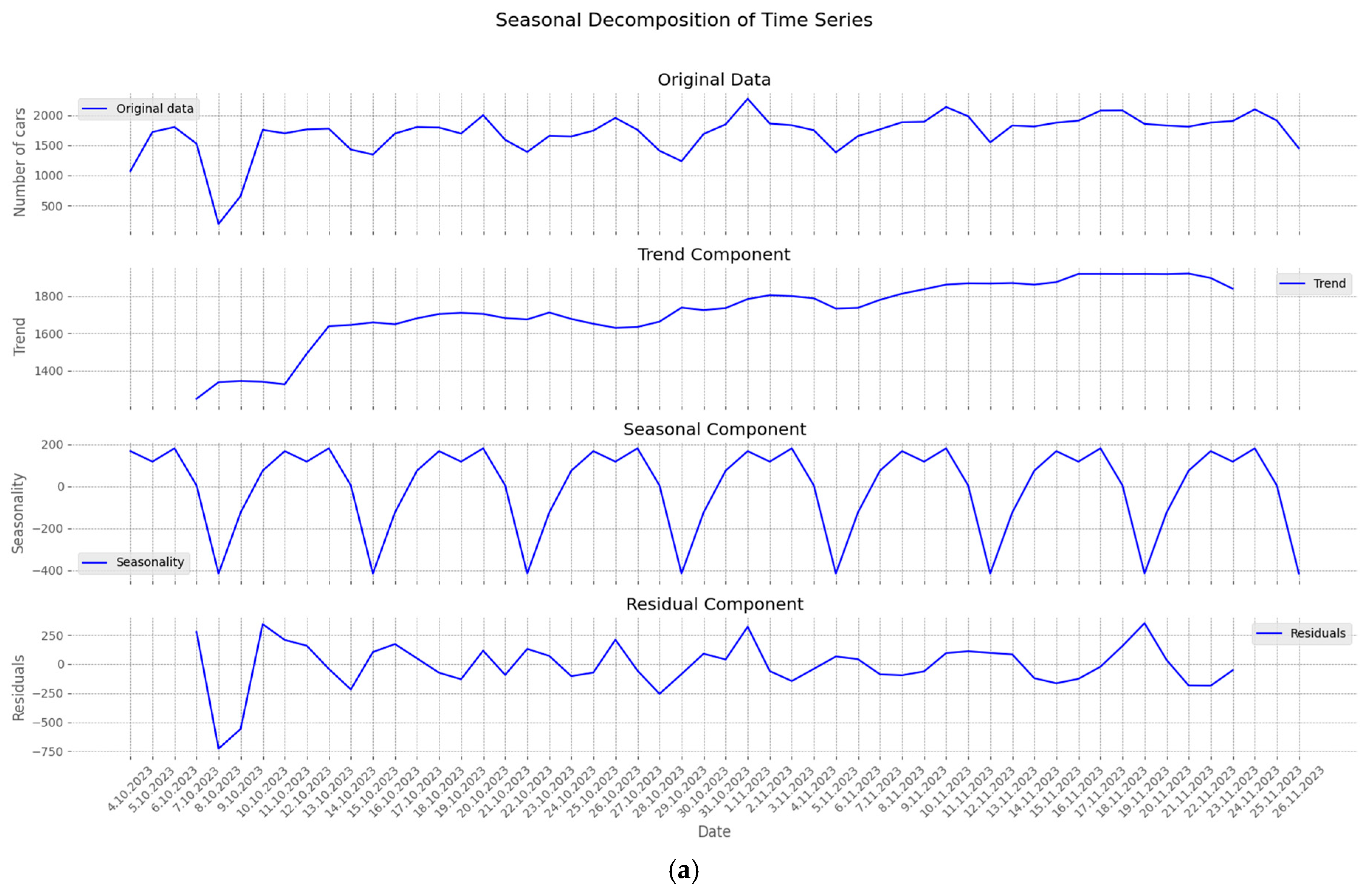
2.2. STL Decomposition

The results of the STL decomposition (Figure 1) reveal the key components of the time series representing the number of vehicles (along the ordinate) over a given period (along the abscissa).

The first graph of both figures presents the original data. The long-term trend (second graph) of the first dataset initially shows a decline, followed by relative stability and a slight increase. Toward the end of the analyzed period, another decrease is observed. The trend of the second dataset looks much more unstable. The season graph (third graph) of both datasets exhibits a clearly defined weekly seasonality, suggesting that the number of vehicles follows regular fluctuations throughout the week. The alternation of positive and negative trend values reflects the cyclical nature of the data. The amplitude of seasonal variations remains relatively constant, indicating stability in the recurring patterns. The residual values (last graph) are fairly evenly distributed around zero, demonstrating the effectiveness of the STL decomposition. However, some sharp deviations are observed, which may indicate anomalies, external influences, or noise in the data.

3. ARIMA and SARIMA Configuration and Comparison

3.1. ADF and KPSS Tests

The ARIMA model is assessed for stationarity using the ADF test and KPSS test. The ADF test indicates that the second dataset is nonstationary (p-value > 0.05), requiring first-order differencing, while the first dataset is stationary (p-value < 0.05). After differentiation, the p-value of the ADF test decreases below 0.05, confirming stationarity. The KPSS test indicates stationarity in both datasets (p-value > 0.05) (

Table 1. p-values of ADF and KPSS tests for both datasets.

	1st Dataset p-Value	2nd Dataset p-Value
ADF test before differentiation	0.041	0.25
ADF test after differentiation	4.93 × 10−8	0.044
KPSS test before differentiation	0.1	0.1
KPSS test after differentiation	0.1	0.1

).

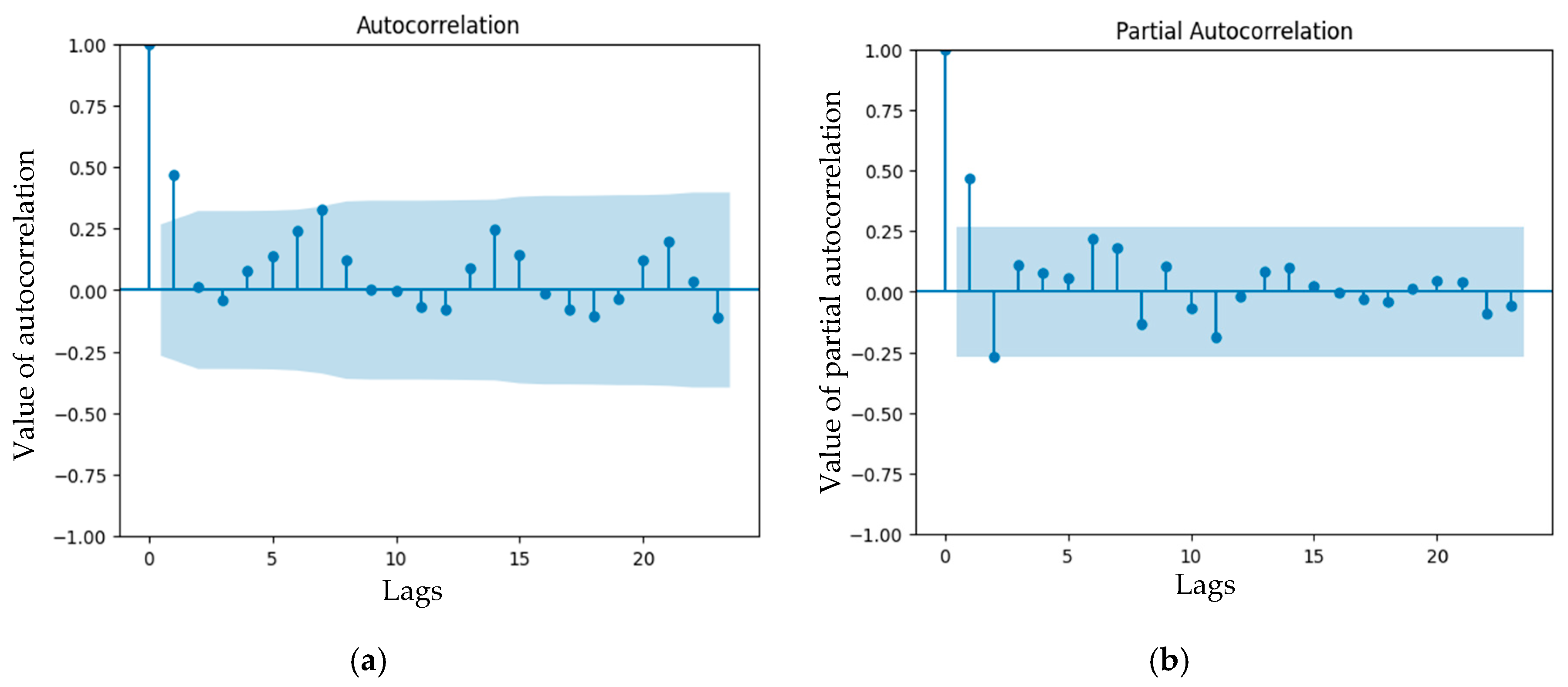
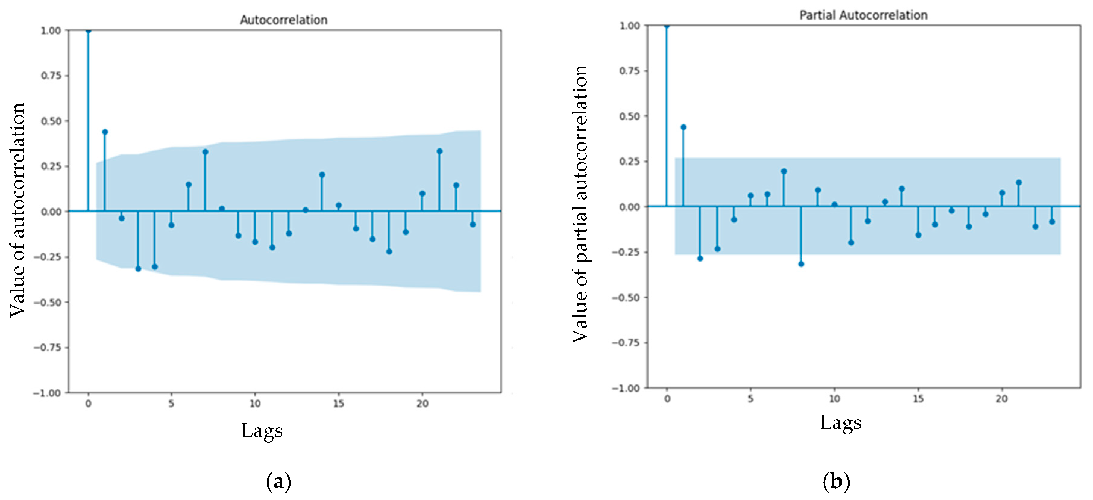
3.2. Analysis of ACF and PACF

The autocorrelation function (ACF) and partial autocorrelation function (PACF) plots (Figure 2, Figure 3, Figure 4 and Figure 5) help determine the model parameters. For all figures, the abscissa represents the number of lag—time steps the series is shifted to compare it with itself, and the ordinate represents the value of correlation or partial autocorrelation at each lag.

The ACF of the first dataset shows increases in the first and second lags. The PACF also shows increases in the first and second lags. Therefore, configurations ARIMA(p = 1, d = 0, q = 1), ARIMA(p = 1, d = 0, q = 2), ARIMA(p = 2, d = 0, q = 1) and ARIMA(p = 2, d = 0, q = 2) should be investigated. The periodical peaks show a periodicity with period 7, which indicates SARIMA (P = 1, D = 0, Q = 1, m = 7), SARIMA (P = 1, D = 0, Q = 2, m = 7), SARIMA (P = 2, D = 0, Q = 1, m = 7), and SARIMA (P = 2, D = 0, Q = 2, m = 7) should be investigated.

The ACF of the first dataset after differencing shows increases in the first and third lags. The PACF also show increases in the first and third lags Therefore, configurations ARIMA(p = 1, d = 1, q = 1), ARIMA(p = 3, d = 1, q = 3), ARIMA(p = 1, d = 1, q = 3), and ARIMA(p = 3, d = 1, q = 1) should be investigated. The periodical peaks show a periodicity with period 7, which indicates SARIMA (P = 1, D = 0, Q = 1, S = 7), SARIMA (P = 1, D = 0, Q = 3, S = 7), SARIMA (P = 3, D = 0, Q = 1, S = 7), and SARIMA (P = 3, D = 0, Q = 3, S = 7) should be investigated.

The ACF of the second dataset shows increases in the first and second lag. The PACF shows increases in the first and second lags. Therefore, configurations ARIMA(p = 1, d = 0, q = 1), ARIMA(p = 2, d = 0, q = 2),ARIMA(p = 1, d = 0, q = 2), and ARIMA(p = 2, d = 0, q = 1) should be investigated. The periodical peaks show a periodicity with period 7, which indicates SARIMA (P = 1, D = 0, Q = 1, S = 7), SARIMA (P = 1, D = 0, Q = 2, m = 7), SARIMA (P = 2, D = 0, Q = 1, m = 7), and SARIMA (P = 2, D = 0, Q = 2, m = 7) should be investigated.

Second dataset—first differentiation

The ACF of the second dataset after differentiation shows increases in the first and second lags. The PACF shows increases in the first, second, and third lags. Therefore, configurations (p = 1, d = 1, q = 1), (p = 2, d = 1, q = 2), (p = 1, d = 1, q = 2), (p = 1, d = 1, q = 3), (p = 2, d = 1, q = 3), (p = 3, d = 1, q = 2), and (p = 2, d = 1, q = 1) should be investigated. The periodical peaks show a periodicity with period 7, which indicates SARIMA (P = 1, D = 0, Q = 1, S = 7), SARIMA (P = 1, D = 0, Q = 2, m = 7), SARIMA (P = 2, D = 0, Q = 1, m = 7), and SARIMA (P = 2, D = 0, Q = 2, m = 7) should be investigated.

3.3. Comparison of MAE, MAPE, and RMSE of Different Configurations of ARIMA

Table 2. MAE, MAPE, and RMSE of different ARIMA configurations.

		(1,0,1)	(1,0,2)	(2,0,1)	(2,0,2)	(1,1,1)	(1,1,3)	(3,1,1)	(3,1,3)	(2,1,1)	(1,1,2)	(2,1,2)	(3,1,2)	(2,1,3)
1st dataset	MAE	147.85	153.17	139.07	143.68	185.48	195.08	224.87	220.16	227.58	150.17	219.69	137.06	216.25
	MPE	7.82	8.11	7.27	7.56	10.56	11.5	12.88	12.60	13.08	7.86	12.59	7.06	12.30
	RMSE	244.73	250.68	242.20	242.89	244.68	264.16	280.98	283.08	282.62	247.88	281.06	241.00	280.09
2nd dataset	MAE	129.37	115.19	244.08	262.88	153.83	127.19	147.64	415.83	99.91	132.73	136.21	98.88	123.21
	MPE	7.86	7.26	14.22	15.77	9.22	7.73	8.77	24.62	6.19	8.04	8.16	6.11	7.50
	RMSE	142.52	148.38	265.32	290.56	166.30	139.93	178.24	505.99	123.45	144.59	152.50	121.46	137.91

shows the ARIMA configurations extracted from the analysis of the ACF and PACF in Section 3.2. The mean absolute error (MAE), mean absolute percentage error (MAPE), and root mean squared error (RMSE) indicate that ARIMA (3,1,2) provides the best balance between accuracy and complexity. Configurations (1,0,2) and (1,1,2) also give relatively good values of the MAE, MPE, and RMSE and could be used for further analysis.

3.4. Comparison of MAE, MAPE, and RMSE of Different Configurations of SARIMA

Table 3. MAE, MAPE, and RMSE of different SARIMA configurations.

		(3,1,2), (1,0,1,7)	(1,0,2) (1,0,1,7)	(1,1,2) (1,0,1,7)	(3,1,2), (1,0,2,7)	(1,0,2) (1,0,2,7)	(1,1,2) (1,0,2,7)	(3,1,2) (2,0,1,7)	(1,0,2), (2,0,1,7)	(1,1,2) (2,0,1,7)	(3,1,2) (2,0,2,7)	(1,0,2), (2,0,2,7)	(1,1,2) (2,0,2,7)
First dataset	MAE	221.67	186.11	153.95	257.03	217.62	155.60	246.65	230.04	142.60	260.89	168.92	134.41
	MPE	13.05	10.94	8.65	15.27	12.91	8.78	14.62	13.71	7.82	15.52	9.74	7.30
	RMSE	258.55	222.53	190.97	280.09	242.26	192.46	273.30	250.67	189.65	280.61	207.74	192.33
Second dataset	MAE	116.41	186.39	102.47	136.82	263.68	132.75	124.53	237.97	119.77	164.85	273.17	145.87
	MPE	7.22	11.15	6.38	8.44	15.70	8.20	7.71	14.17	7.41	10.19	16.24	8.99
	RMSE	147.20	198.73	127.91	162.43	299.49	154.70	153.16	262.64	141.86	193.91	308.40	166.68

presents the MAE, MAPE, and RMSE for p, d, and q extracted from the ARIMA analysis (configurations that give minimal error (3,1,2), (1,0,2), and (1,1,2)) and P, D, and Q according to the analysis of the ACF and PACF. Configurations (1,1,2) and (2,0,1,7) show the best result for both datasets. However, the best result for ARIMA (3,1,2) shows a smaller error.

4. Conclusions

After preliminary processing and aggregation, the two datasets acquired from the surveillance traffic system of the Technical University Sofia, branch Plovdiv, are used for the adjustment and evaluation of ARIMA and SARIMA algorithms.

The STL analysis confirms the presence of seasonality and trend variations in the number of vehicles. The observed anomalies in the residual component suggest potential external factors that require further investigation. Considering the research context, it can be hypothesized that the residual component may be influenced by sensor measurement errors and the effect of public holidays.

The analysis and testing demonstrate that ARIMA (3,1,2) and SARIMA (1,1,2)(2,0,1,7) show minimal values of MAE, MPE, and RMSE. Based on the performed test, it could be concluded that even though SARIMA shows satisfactory results, the predicting error with ARIMA is smaller. Therefore, inaccuracies caused by measurement errors and the influence of public holidays are sufficient to reduce the influence of seasonality.

In future works, it would be interesting to compare the experiment with data from other periods as well as to conduct studies with a different granularity of data, for example, hourly load.

In the future, it would be useful to accumulate the extracted data in a public database that would include both the original and aggregated data. This would help a number of studies related to transport safety and efficiency.

References

1. Galkaduwa, C.; Ranasinghe, N. Data Science and Its Importance. Biomed. Sci. Clin. Res. 2024, 3, 1–4. [Google Scholar]
2. Lukas, S.; Uhrina, M.; Frnda, J. UHD Database Focus on Smart Cities and Smart Transport. Electronics 2024, 13, 904. [Google Scholar] [CrossRef]
3. Chattopadhyay, A.; Lee, C.Y.; Lee, Y.C.; Liu, C.L.; Chen, H.K.; Li, Y.H.; Chuang, E.Y. Twnbiome: A public database of the healthy Taiwanese gut microbiome. BMC Bioinform. 2024, 24, 474. [Google Scholar] [CrossRef] [PubMed]
4. Szostek, K.; Mazur, D.; Drałus, G.; Kusznier, J. Analysis of the Effectiveness of ARIMA, SARIMA, and SVR Models in Time Series Forecasting: A Case Study of Wind Farm Energy Production. Energies 2024, 17, 4803. [Google Scholar] [CrossRef]
5. Santoso, A.B.; Widodo, T. Predicting the number of forest and land fire hotspot occurrences using the arima and sarima methods. J. Sisfokom. 2024, 13, 119–129. [Google Scholar] [CrossRef]
6. Hyndman, R.; Athanasopoulos, G. Forecasting: Principles and Practice; Monash University: Melbourne, VIC, Australia, 2021; Available online: https://otexts.com/fpp3/ (accessed on 7 May 2025).
Figure 1. STL decomposition: (a) first dataset; (b) second dataset.
Engproc 100 00029 g001aEngproc 100 00029 g001b
Figure 2. ACF and PACF of original dataset 1: (a) ACF; (b)PACF.
Engproc 100 00029 g002
Figure 3. ACF and PACF of dataset 1 after differentiation: (a) ACF; (b) PACF.
Engproc 100 00029 g003
Figure 4. ACF and PACF of original dataset 2: (a) ACF; (b) PACF.
Engproc 100 00029 g004
Figure 5. ACF and PACF of dataset 2 after differentiation: (a) ACF; (b) PACF.
Engproc 100 00029 g005