Hydrogen Atom as a Nonlinear Oscillator Under Circularly Polarized Light: Epicyclical Electron Orbits

Abstract

We used Clifford algebra $C{l}_{2,0}$ to find the 2D orbit of a hydrogen electron under a Coulomb force and a perturbing circularly polarized electric field of light at angular frequency $\omega$, which is turned on at time $t=0$ via a unit step switch. Using a coordinate system co-rotating with the electron’s unperturbed circular orbit at angular frequency ${\omega }_0$, we derived a complex differential equation that is similar to but different from that of the Lorentz oscillator equation for light–atom interaction. We solved the homogeneous and particular differential equation and showed that the position of the electron is a linear combination of five exponential Fourier terms or orbital wave functions with frequencies 0, ${\omega }_0$, $2{\omega }_0$, $(2{\omega }_0-\omega )$, and $\omega$, whose coefficients depend on the light-to-atom frequency ratio $\omega /{\omega }_0$ and light-to-atom force magnitude ratio $A/r_0$. We showed that the electron orbits are approximately Keplerian at light-to-atom frequency ratio $\alpha =\omega /{\omega }_0=\{0,1,2\}$, with the orbits becoming discontinuous and divergent as $\alpha \to 1^{\pm }$, but continuous and non-divergent at $\alpha =\{0,2\}$. These Keplerian orbits are approximated by the sum of the zeroth, first, and second harmonics of the electron’s unperturbed orbital wave function ${\widehat{\psi }}_0=e^{\widehat{\mathsf{ı}}{\omega }_{0}t}$, corresponding to the eccentric, deferent, and epicycle in the Copernican construction of planetary orbits.

1. Introduction

The two-dimensional (2D) interaction between a hydrogen atom and a circularly polarized (CP) light may be expressed as a force equation relating the position $\mathbf{r}$ of the electron with respect to the massive proton at the origin and electric field $\mathbf{E}$ of light:

$$\ddot{\mathbf{r}}=-k{\displaystyle \frac{\mathbf{r}}{{\left|\mathbf{r}\right|}^3}}-{\displaystyle \frac{q}{m}}\mathbf{E},$$

(1)

where k is the electrostatic force constant, q is the magnitude of electron charge, and m is the electron mass. This equation is nonlinear and has no known closed-form analytical solution, especially for time-varying electric field $\mathbf{E}$.

One reason for this absence of analytical solution is that the CP problem belongs to a class of difficult problems: the restricted three-body problem [1]. Some restricted three-body problems are the orbits of the Moon under the gravitational force of the Earth and Sun [2] or the orbits of Trojan asteroids under the gravitational force of the Sun and Jupiter [3]. For our case, our problem is to find the orbit of an electron under the influence of a massive proton and an electric force of a circularly polarized light. This problem is similar to the motion of a dust particle around a planet far from the Sun [4].

The CP problem may be difficult to solve analytically, but it provides a framework for classically interpreting the experiments on the ionization of hydrogen atoms by circularly polarized radiation (e.g., microwaves) [5,6,7,8,9]. That is why numerous attempts have been made to shed some light on the problem, usually via Hamiltonian analysis. For example, some authors construct the Hamiltonian of the system, derive the Hamiltonian in a coordinate system co-rotating with the frequency $\omega$ of the incident light, average out the fast oscillations, draw phase plots to analyze stable points, or analyze zero-velocity surfaces [10,11,12,13,14,15,16,17,18,19,20]. Other authors use the Hamiltonian to derive the equations of motion and use computational and analytical techniques (e.g., the Runge–Kutta algorithm, Kustaanheimo–Steifel transformation, and action-angle variables) to draw the orbits or compute the binding energies and ionization probabilities [13,14,18,19,21,22,23,24,25,26,27,28,29,30,31]. And other authors used the Hamiltonian to analytically determine the precession frequencies of the Keplerian orbit of the electron [32,33].

The Hamiltonian approach rests on the assumption that scalars are easier to handle than vectors. This is true if there are constants in the motion, such as energy. But for the CP problem, energy is not constant in time [34]. Also, since the orbits appear to be epicyclical, complex numbers and 2D vectors would be a more direct approach for two reasons: (1) epicyclical orbits can be expressed as a sum of vectors rotating at different frequencies, and (2) Copernican and Ptolemaic epicycles in Celestial Mechanics are best described in terms of exponential Fourier series in Complex Analysis [35]. But can we combine vectors and complex numbers in a single mathematical formalism?

To answer this need for a unified mathematical formalism, we propose the Clifford (geometric) algebra $\mathcal{C}{\ell }_{2,0}$ [36,37,38,39,40,41,42], which has not been used before to solve the light–atom interaction equation in Equation (1). In this algebra, the square of orthonormal unit vectors ${\mathbf{e}}_1$ and ${\mathbf{e}}_2$ are equal to unity or normalized to unit length, while their product anticommutes due to the orthogonality of the two vectors. From this orthonormality axiom, we can show that if we define the unit bivector $\widehat{\mathsf{ı}}\equiv {\mathbf{e}}_1{\mathbf{e}}_2$, then $\widehat{\mathsf{ı}}$ is an imaginary number that anticommutes with unit vectors ${\mathbf{e}}_1$ and ${\mathbf{e}}_2$. All theorems of 2D Vector Algebra [43] and of Complex Analysis [44] can be used in Clifford Algebra $C{l}_{2,0}$, though there are some theorems such as ${\mathbf{e}}_1\widehat{\mathsf{ı}}={\mathbf{e}}_2$ and ${\mathbf{e}}_2\widehat{\mathsf{ı}}=-{\mathbf{e}}_1$ that are unique to $C{l}_{2,0}$: the right-multiplication of the bivector $\widehat{\mathsf{ı}}$ to the unit vector ${\mathbf{e}}_1$ and ${\mathbf{e}}_2$ rotates these vectors counterclockwise by $\pi /2$. In the usual complex vector analysis, the imaginary number i commutes with the vectors ${\mathbf{e}}_1$ and ${\mathbf{e}}_2$, so that ${\mathbf{e}}_{1}i$ and ${\mathbf{e}}_{2}i$ are simply imaginary vectors.

Thus, since we are going to use vectors in Clifford Algebra $C{l}_{2,0}$, we shall not use the Hamiltonian approach via scalar kinetic and potential energies, but the Newtonian approach via force and acceleration vectors as given in Equation (1). To simplify this force–acceleration equation, we shall assume that the electric field $\mathbf{E}$ of the circularly polarized light is much weaker than the Coulomb field. We shall assume that the light is switched on at $t=0$ and never turned off. That is, we shall define our switch as a Heaviside unit-step function [45], and not some other more complicated switch function [8,13,21,22,23]. We shall assume that the electron is initially in a uniform circular motion around the massive proton (fixed at the origin) just before the light is switched on. We shall assume that the electric field $\mathbf{E}$ of light lies in the orbital plane of the electron, so that the 3D problem is reduced to 2D. On the other hand, we shall not assume a frictional damping force proportional to the velocity $\mathbf{v}=\dot{\mathbf{r}}$ or a radiation damping force proportional to the jerk $\stackrel{⃛}{\mathbf{r}}=\ddot{\mathbf{v}}=\dot{\mathbf{a}}$ [46,47,48,49,50,51,52,53,54,55,56,57,58]. We shall also not take into account the force $-q\dot{\mathbf{r}}\times \mathbf{B}$ of the circularly polarized magnetic field $\mathbf{B}$ of light [33,50,51,52,53,55].

Given these assumptions, we may now rephrase our problem as follows: what is the resulting orbit of the hydrogen electron after the circularly polarized light is switched on? Because this is a classical problem, we cannot assume that the electron simply jumps to a new orbit with a different radius, as given in the Bohr–Sommerfeld model of the atom [59]. Instead, we shall assume that the position $\mathbf{r}$ and the velocity $\mathbf{v}=\dot{\mathbf{r}}$ are continuous just before and just after the light is switched on at time $t=0$. We shall also assume that the electric field $\mathbf{E}$ of a circularly polarized light on the electron is much weaker compared to Coulomb field due to the proton, so that we can use the methods of perturbation theory [60] and solve the resulting differential equation using the exponential Fourier analysis.

We have also tried to solve this problem before in our previous paper [61], but we made a mistake in the sign of the exponential: we wrote ${\widehat{c}}_{-1}=-3e^{-2{\varphi }_0\widehat{\mathsf{ı}}}{\widehat{c}}_1^{\ast }$, where ${\varphi }_0$ is the orbital phase of the electron’s unperturbed orbit just before the circularly polarized light is switched on. This equation should have been written as ${\widehat{c}}_{-1}=-3e^{2{\varphi }_0\widehat{\mathsf{ı}}}{\widehat{c}}_1^{\ast }$, which agrees with the Copernican eccentric–epicycle relation for planetary orbits [42].

Our conclusion then was that the electron orbits are all divergent at the three resonant light-to-atom frequency ratios: $\alpha =\omega /{\omega }_0=\{0,1,2\}$. We shall correct this conclusion in our present paper: the orbit is discontinuous and divergent at $\alpha =1$, but finite and quasi-Keplerian at $\alpha =\{0,2\}$. In addition, we shall provide actual plots of the orbits instead of simply identifying parts of the exponential Fourier terms in terms of the Copernican notions of eccentric, deferent, and epicycle. Specifically, we shall plot the orbits at different light-to-atom frequency ratios subject to the phase condition ${\varphi }_0=\delta =0$, where $\delta$ is the phase of the electric field $\mathbf{E}$ of the circularly polarized light.

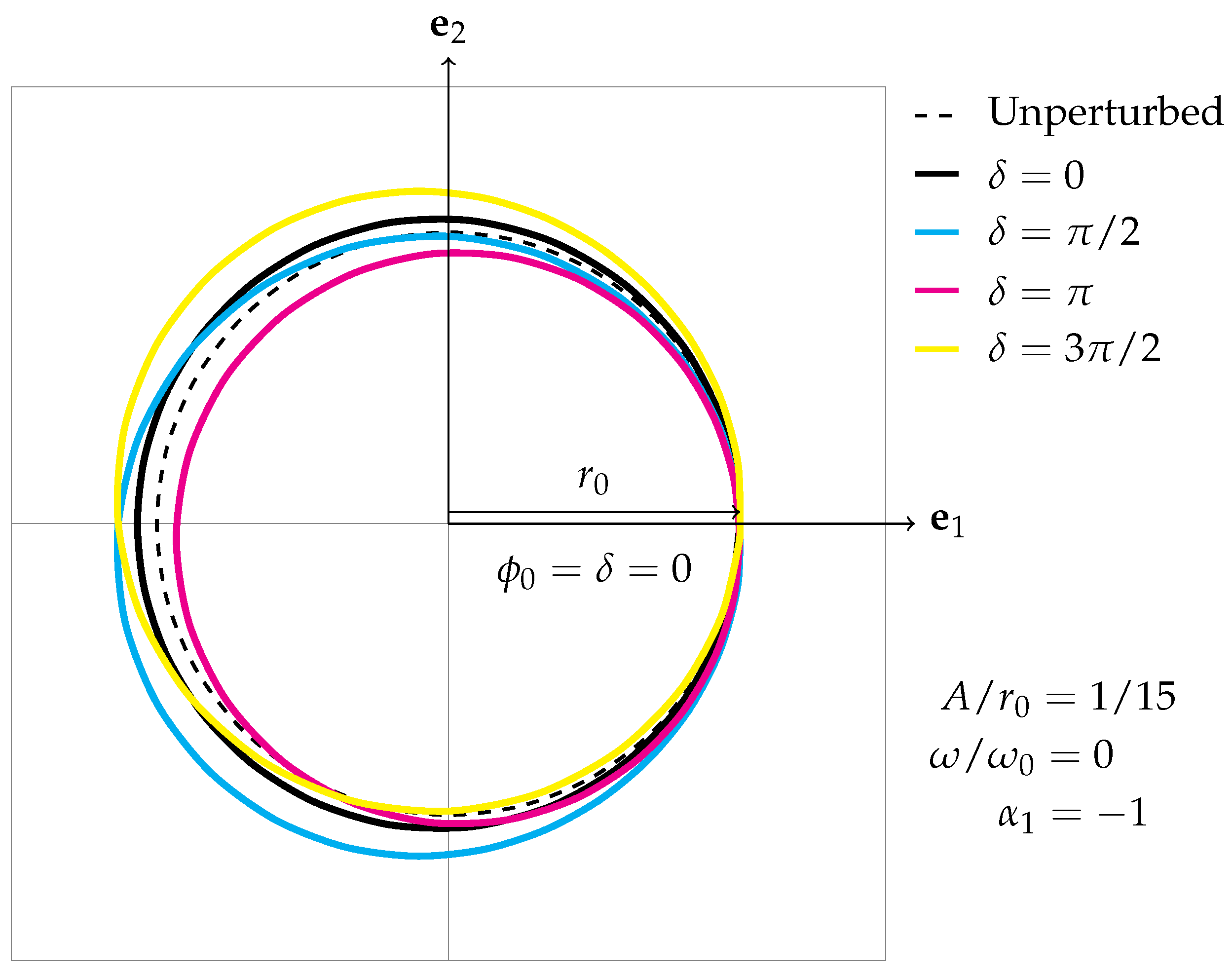
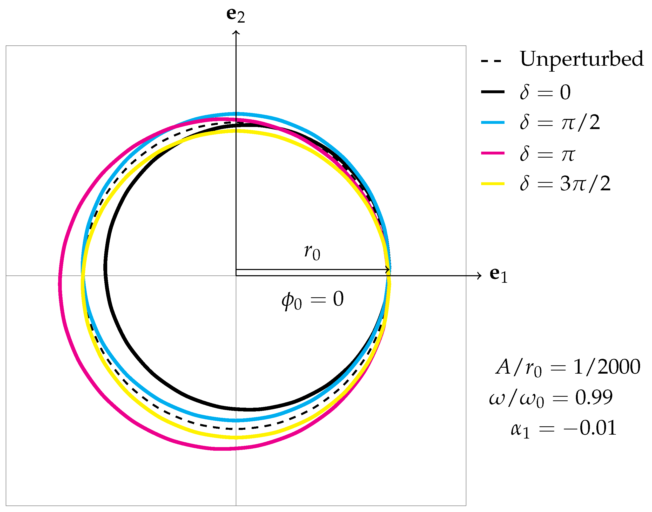
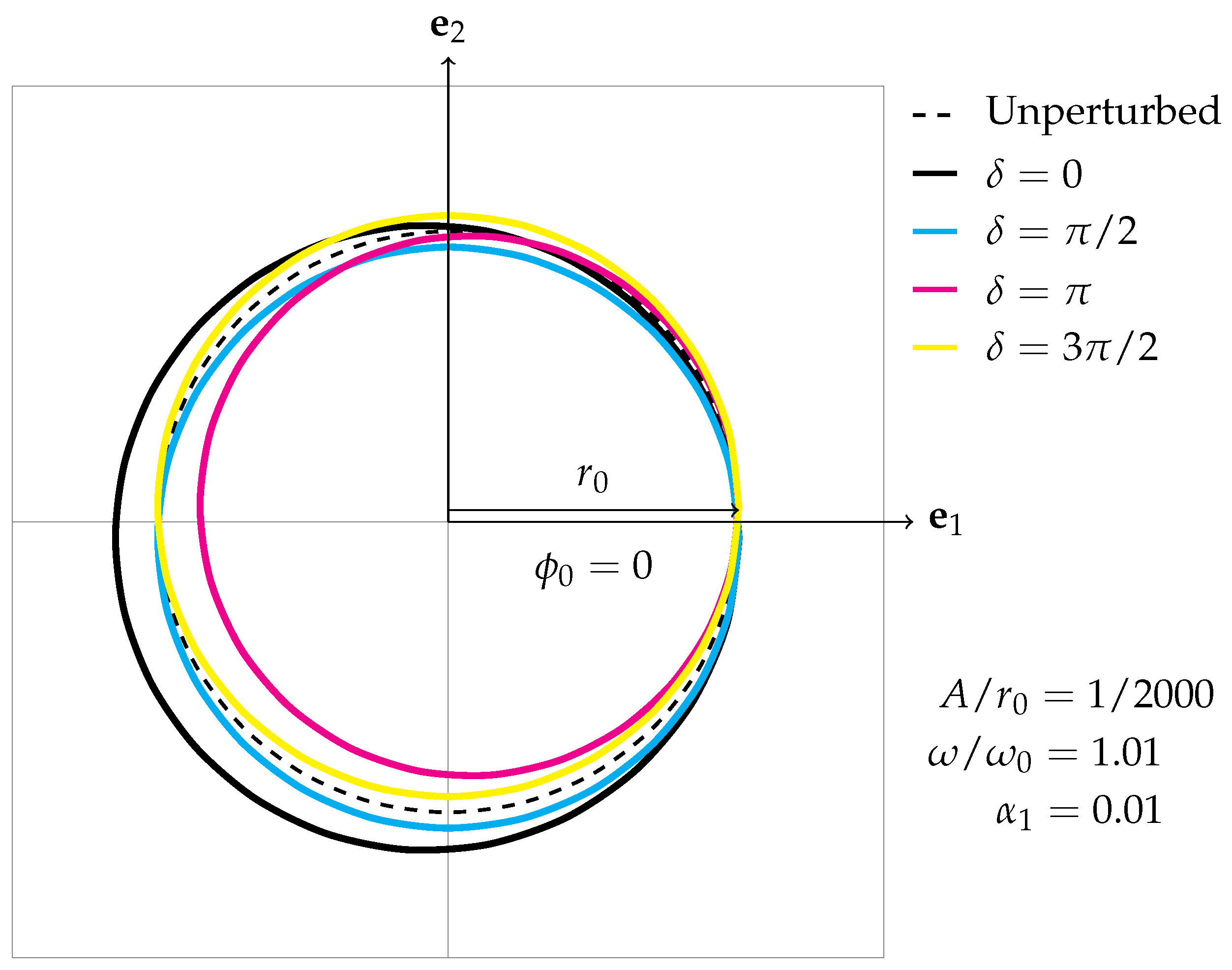
And for resonant and near-resonant light-to-atom frequency ratios, we shall plot the orbits for ${\varphi }_0=0$, but setting $\delta =\{0,\pi /2,\pi ,3\pi /2\}$.

We shall divide our paper into five sections. Section 1 is the Introduction. In Section 2, we shall discuss the fundamental axioms and theorems of Clifford geometric algebra $C{l}_{2,0}$ as a complex vector algebra, following the notation in Ref. [42]. In Section 3, we shall derive the nonlinear differential equation in complex form for a hydrogen electron perturbed from its initial circular orbit by a circularly polarized light, and then find the homogeneous and particular solutions of this equation. In Section 4, we shall impose the continuity of position and velocity when the light is switched on at time $t=0$ to find the homogeneous coefficients in terms of the amplitude $\widehat{a}=a{e}^{\widehat{\mathsf{ı}}\delta }$ of the circularly polarized light. We shall express the position of the electron as a linear combination of the five exponential Fourier terms, which we shall interpret as a vector sum of the eccentric, deferent, and three epicycles, as similarly done in the Copernican celestial model. We shall compute the values of the exponential Fourier coefficients at different light-to-atom frequency ratios and phase values, then plot the resulting representative orbits. Section 5 is the Conclusions.

2. Clifford Algebra

In this section, we shall discuss the important axioms and theorems of Clifford (geometric) algebra $C{l}_{2,0}$ and show how this algebra combines vectors and complex numbers in a single formalism. In particular, we shall show how Euler’s identity can be used to rotate vectors—a theorem that will become important later in the description of circular orbits and circularly polarized light. Our discussion and notations shall follow that of Ref. [42].

2.1. Vectors and Imaginary Numbers

Let ${\mathbf{e}}_1$ and ${\mathbf{e}}_2$ be two vectors that satisfy the orthonormality relations in Clifford geometric algebra $\mathcal{C}{l}_{2,0}$:

$$\begin{array}{cc}\hfill {\mathbf{e}}_1^2& ={\mathbf{e}}_2^2=1,\hfill \end{array}$$

(2a)

$$\begin{array}{cc}\hfill {\mathbf{e}}_1{\mathbf{e}}_2& =-{\mathbf{e}}_2{\mathbf{e}}_1.\hfill \end{array}$$

(2b)

That is, ${\mathbf{e}}_1$ and ${\mathbf{e}}_2$ are unit vectors that anticommute. If we define the unit bivector $\widehat{\mathsf{ı}}$ as

$$\widehat{\mathsf{ı}}={\mathbf{e}}_1{\mathbf{e}}_2,$$

(3)

we can use the orthonormality relations together with the associativity property of vector products to obtain

$${\widehat{\mathsf{ı}}}^2=-1,$$

(4)

and

$$\begin{array}{cc}\hfill {\mathbf{e}}_1\widehat{\mathsf{ı}}& =-\widehat{\mathsf{ı}}{\mathbf{e}}_1={\mathbf{e}}_2,\hfill \end{array}$$

(5a)

$$\begin{array}{cc}\hfill {\mathbf{e}}_2\widehat{\mathsf{ı}}& =-\widehat{\mathsf{ı}}{\mathbf{e}}_2=-{\mathbf{e}}_1.\hfill \end{array}$$

(5b)

Notice that $\widehat{\mathsf{ı}}$ is a unit imaginary that anticommutes with vectors ${\mathbf{e}}_1$ and ${\mathbf{e}}_2$, unlike in the complexified vector algebra where the imaginary number i is treated as a scalar that commutes with vectors.

2.2. Vector Products and Complex Numbers

Let $\mathbf{a}$ and $\mathbf{b}$ be two vectors in Clifford algebra $C{l}_{2,0}$:

$$\begin{array}{cc}\hfill \mathbf{a}& =a_1{\mathbf{e}}_1+a_2{\mathbf{e}}_2,\hfill \end{array}$$

(6a)

$$\begin{array}{cc}\hfill \mathbf{b}& =b_1{\mathbf{e}}_1+b_2{\mathbf{e}}_2,\hfill \end{array}$$

(6b)

where $a_1$, $a_2$, $b_1$, and $b_2$ are their scalar components. The geometric product of these two vectors may be expressed as

$$\mathbf{a}\mathbf{b}=\mathbf{a}·\mathbf{b}+\mathbf{a}\wedge \mathbf{b},$$

(7)

where

$$\begin{array}{cc}\hfill \mathbf{a}·\mathbf{b}& =a_1{b}_1+a_2{b}_2,\hfill \end{array}$$

(8a)

$$\begin{array}{cc}\hfill \mathbf{a}\wedge \mathbf{b}& =(a_1{b}_2-a_2{b}_1)\widehat{\mathsf{ı}}\hfill \end{array}$$

(8b)

are the inner (dot) and outer (wedge) products, respectively. Notice that the product $\mathbf{a}\mathbf{b}$ is a complex number (or a scalar-bivector cliffor). Also, notice that these definitions allow us to define the dot and wedge products in terms of the anticommutator and commutator of $\mathbf{a}$ and $\mathbf{b}$:

$$\begin{array}{cc}\hfill \mathbf{a}·\mathbf{b}& ={\displaystyle \frac{1}{2}}(\mathbf{a}\mathbf{b}+\mathbf{b}\mathbf{a}),\hfill \end{array}$$

(9a)

$$\begin{array}{cc}\hfill \mathbf{a}\wedge \mathbf{b}& ={\displaystyle \frac{1}{2}}(\mathbf{a}\mathbf{b}-\mathbf{b}\mathbf{a}).\hfill \end{array}$$

(9b)

In order to facilitate the smooth transition from vectors to complex numbers and vice versa, we use the identities in Equation (5a,b) to rewrite the expressions for vectors $\mathbf{a}$ and $\mathbf{b}$ into

$$\begin{array}{cc}\hfill \mathbf{a}& ={\mathbf{e}}_1\widehat{a}={\widehat{a}}^{\ast }{\mathbf{e}}_1,\hfill \end{array}$$

(10a)

$$\begin{array}{cc}\hfill \mathbf{b}& ={\mathbf{e}}_1\widehat{b}={\widehat{b}}^{\ast }{\mathbf{e}}_1,\hfill \end{array}$$

(10b)

where

$$\begin{array}{cc}\hfill \widehat{a}& =a_1+a_2\widehat{\mathsf{ı}},\hfill \end{array}$$

(11a)

$$\begin{array}{cc}\hfill a^{\ast }& =a_1-a_2\widehat{\mathsf{ı}}\hfill \end{array}$$

(11b)

$$\begin{array}{cc}\hfill \widehat{b}& =b_1+b_2\widehat{\mathsf{ı}},\hfill \end{array}$$

(11c)

$$\begin{array}{cc}\hfill {\widehat{b}}^{\ast }& =b_1-b_2\widehat{\mathsf{ı}}\hfill \end{array}$$

(11d)

are complex numbers (or scalar-bivector cliffors) and their corresponding complex conjugates (denoted by *).

The relations in Equation (10a,b) let us express the geometric products $\mathbf{a}\mathbf{b}$ and $\mathbf{b}\mathbf{a}$ as

$$\begin{array}{cc}\hfill \mathbf{a}\mathbf{b}& ={\mathbf{e}}_1\widehat{a}{\mathbf{e}}_1\widehat{b}={\mathbf{e}}_1{\mathbf{e}}_1{\widehat{a}}^{\ast }\widehat{b}={\widehat{a}}^{\ast }\widehat{b},\hfill \end{array}$$

(12a)

$$\begin{array}{cc}\hfill \mathbf{b}\mathbf{a}& ={\mathbf{e}}_1\widehat{b}{\mathbf{e}}_1\widehat{a}={\mathbf{e}}_1{\mathbf{e}}_1{\widehat{b}}^{\ast }\widehat{a}={\widehat{b}}^{\ast }\widehat{a},\hfill \end{array}$$

(12b)

which allow us to rewrite the expressions for $\mathbf{a}·\mathbf{b}$ and $\mathbf{a}\wedge \mathbf{b}$ in Equation (9a,b) into complex form:

$$\begin{array}{cc}\hfill \mathbf{a}·\mathbf{b}& ={\displaystyle \frac{1}{2}}\left({\widehat{a}}^{\ast }\widehat{b}+{\widehat{b}}^{\ast }\widehat{a}\right),\hfill \end{array}$$

(13a)

$$\begin{array}{cc}\hfill \mathbf{a}\wedge \mathbf{b}& ={\displaystyle \frac{1}{2}}\left({\widehat{a}}^{\ast }\widehat{b}-{\widehat{b}}^{\ast }\widehat{a}\right).\hfill \end{array}$$

(13b)

Thus, the products $\mathbf{a}·\mathbf{b}$ and $\mathbf{a}\wedge \mathbf{b}$ are related to the commutator and anticommutator of ${\widehat{a}}^{\ast }\widehat{b}$ and ${\widehat{b}}^{\ast }\widehat{a}$, respectively.

If we set $\mathbf{a}=\mathbf{b}$ in Equation (12a), then

$${\mathbf{a}}^2={\widehat{a}}^{\ast }\widehat{a}=|\widehat{a}{|}^2={\left|\mathbf{a}\right|}^2.$$

(14)

That is, the square of the length of a vector $\mathbf{a}$ is equal to the product of the complex number $\widehat{a}$ and its complex conjugate ${\widehat{a}}^{\ast }$. In ordinary vector analysis, the square ${\mathbf{a}}^2$ is not defined, so that the normal notation should have been $\mathbf{a}·\mathbf{a}={\widehat{a}}^{\ast }\widehat{a}$. Even then, this jump from vectors to complex numbers is normally treated as a standard translation between two different mathematical languages (vectors and complex numbers) and not as different forms of the same equation in the same underlying mathematical language (Clifford algebra).

Equation (14) also allows us to define the inverse of a vector $\mathbf{a}$ and its corresponding complex number $\widehat{a}$ as

$$\begin{array}{cc}\hfill {\mathbf{a}}^{-1}& ={\displaystyle \frac{\mathbf{a}}{{\left|\mathbf{a}\right|}^2}},\hfill \end{array}$$

(15a)

$$\begin{array}{cc}\hfill {\widehat{a}}^{-1}& ={\displaystyle \frac{{\widehat{a}}^{\ast }}{|\widehat{a}{|}^2}}.\hfill \end{array}$$

(15b)

Note that the inverse ${\widehat{a}}^{-1}$ is a familiar expression in Complex Analysis, while the inverse ${\mathbf{a}}^{-1}$ is undefined in ordinary vector algebra.

2.3. Vector Rotations and Euler’s Identity

Since ${\widehat{\mathsf{ı}}}^2=-1$, then we may use Euler’s identity to write

$$e^{\pm \widehat{\mathsf{ı}}\varphi }=cos\varphi \pm \widehat{\mathsf{ı}}sin\varphi ,$$

(16)

where $\varphi$ is a real number scalar. Multiplying the exponential from the left by the unit vectors ${\mathbf{e}}_1$ or ${\mathbf{e}}_2$ and using the anticommutation relations in Equation (5a,b), we obtain

$$\begin{array}{cc}\hfill {\mathbf{e}}_1{e}^{\pm \widehat{\mathsf{ı}}\varphi }& ={\mathbf{e}}_{1}cos\varphi \pm {\mathbf{e}}_{2}sin\varphi =e^{\mp \widehat{\mathsf{ı}}\varphi }{\mathbf{e}}_1,\hfill \end{array}$$

(17a)

$$\begin{array}{cc}\hfill {\mathbf{e}}_2{e}^{\pm \widehat{\mathsf{ı}}\varphi }& =\mp {\mathbf{e}}_{1}sin\varphi +{\mathbf{e}}_{2}cos\varphi =e^{\mp \widehat{\mathsf{ı}}\varphi }{\mathbf{e}}_2.\hfill \end{array}$$

(17b)

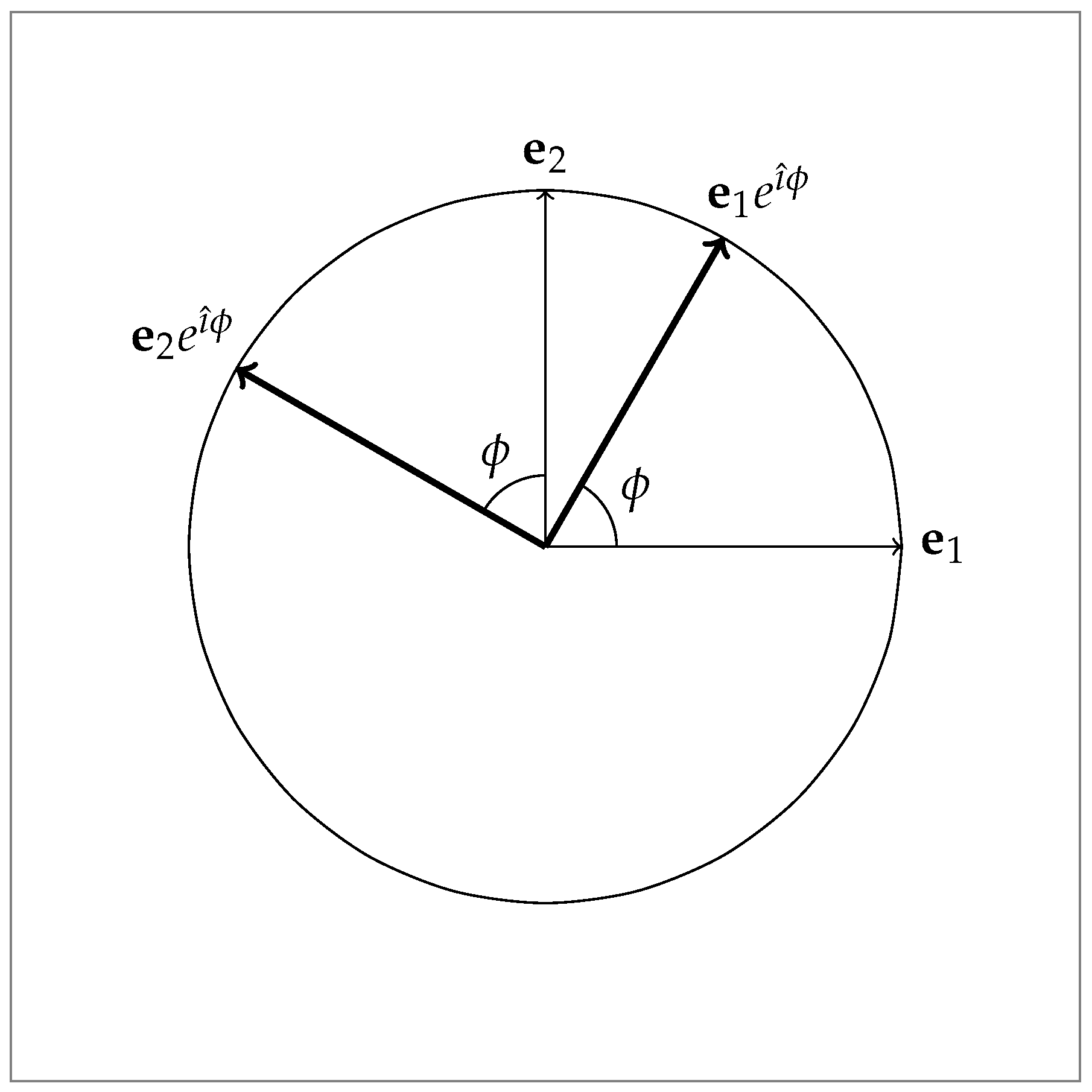
That is, ${\mathbf{e}}_1{e}^{\widehat{\mathsf{ı}}\varphi }$ and ${\mathbf{e}}_2{e}^{\widehat{\mathsf{ı}}\varphi }$ are rotations of ${\mathbf{e}}_1$ and ${\mathbf{e}}_2$ by an angle $\varphi$, respectively. The rotation is counterclockwise if $\varphi >0$ and clockwise if $\varphi <0$.

If the rotation angle is $\varphi =\pi /2$, then

$$\begin{array}{cc}\hfill cos\varphi & =cos{\displaystyle \frac{\pi }{2}}=0,\hfill \end{array}$$

(18a)

$$\begin{array}{cc}\hfill sin\varphi & =sin{\displaystyle \frac{\pi }{2}}=0,\hfill \end{array}$$

(18b)

so that Equations (16) and (17a) reduce to the vector–bivector relations in Equation (5a,b) (see Figure 1). This allows us to geometrically interpret the bivector $\widehat{\mathsf{ı}}=e^{\widehat{\mathsf{ı}}\pi /2}$ as a rotation operator of the unit vectors ${\mathbf{e}}_1$ and ${\mathbf{e}}_2$: left-acting counterclockwise rotation of the said vectors on its left and right-acting clockwise rotation operator of the said vectors on its right.

Using exponential functions, we may express the vectors $\mathbf{a}$ and $\mathbf{b}$ in terms of their polar forms:

$$\begin{array}{cc}\hfill \mathbf{a}& ={\mathbf{e}}_1\widehat{a}={\mathbf{e}}_{1}a{e}^{\widehat{\mathsf{ı}}{\varphi }_a}=a{e}^{-\widehat{\mathsf{ı}}{\varphi }_a}{\mathbf{e}}_1={\widehat{a}}^{\ast }{\mathbf{e}}_1,\hfill \end{array}$$

(19a)

$$\begin{array}{cc}\hfill \mathbf{b}& ={\mathbf{e}}_1\widehat{b}={\mathbf{e}}_{1}b{e}^{\widehat{\mathsf{ı}}{\varphi }_a}=b{e}^{-\widehat{\mathsf{ı}}{\varphi }_b}{\mathbf{e}}_1={\widehat{b}}^{\ast }{\mathbf{e}}_1,\hfill \end{array}$$

(19b)

where a and b are the lengths of vectors $\mathbf{a}$ and $\mathbf{b}$, while ${\varphi }_a$ and ${\varphi }_b$ are their azimuthal angles measured counterclockwise from the direction of ${\mathbf{e}}_1$. The product of vectors $\mathbf{a}$ and $\mathbf{b}$ becomes

$$\mathbf{a}\mathbf{b}={\widehat{a}}^{\ast }\widehat{b}=ab{e}^{i({\varphi }_b-{\varphi }_a)}=ab\left[cos({\varphi }_b-{\varphi }_a)+\widehat{\mathsf{ı}}sin({\varphi }_b-{\varphi }_a)\right].$$

(20)

Separating the scalar and bivector parts yields

$$\begin{array}{c}\hfill \mathbf{a}·\mathbf{b}=abcos({\varphi }_b-{\varphi }_a),\end{array}$$

(21a)

$$\begin{array}{c}\hfill \mathbf{a}\wedge \mathbf{b}=ab\widehat{\mathsf{ı}}sin({\varphi }_b-{\varphi }_a),\end{array}$$

(21b)

which correspond to real and imaginary parts of ${\widehat{a}}^{\ast }\widehat{b}$, respectively.

3. Hydrogen Atom as a Nonlinear Oscillator Under Circularly Polarized Light

In Section 2, we introduced the Clifford algebra $C{l}_{2,0}$. Now in Section 3, we shall use the $C{l}_{2,0}$ formalism to discuss how the two-dimensional interaction of a circularly polarized light and a hydrogen atom leads to a complex nonlinear oscillator equation whose nonlinearity is not due to higher powers of the perturbation, but simply to the presence of the complex conjugate in the perturbation in a coordinate system co-rotating with the unperturbed circular orbit of the electron. We shall solve this complex nonlinear differential equation by finding its homogeneous and particular solutions, and then combine these two solutions to obtain the total solution. To solve for the unknown coefficients, we shall impose that the position and velocity of the electron are continuous just before and just after the circularly polarized light is switched on.

3.1. Circularly Polarized Light

If the electric field $\mathbf{E}$ of light is left-circularly polarized (or rotating counterclockwise) in the plane defined by the unit vectors ${\mathbf{e}}_1$ and ${\mathbf{e}}_2$, then

$$\begin{array}{cc}\hfill \mathbf{E}& ={\mathbf{e}}_1\widehat{E}={\mathbf{e}}_1\widehat{a}\widehat{\psi }={\mathbf{e}}_{1}a{e}^{\widehat{\mathsf{ı}}(\omega t+\delta )},\hfill \end{array}$$

(22)

where the electric field amplitude $\widehat{a}$ and the wave function $\widehat{\psi }$ are given by

$$\begin{array}{cc}\hfill \widehat{a}& =a{e}^{\widehat{\mathsf{ı}}\delta },\hfill \end{array}$$

(23a)

$$\begin{array}{cc}\hfill \widehat{\psi }& =e^{\widehat{\mathsf{ı}}\omega t},\hfill \end{array}$$

(23b)

with a, $\delta$, and $\omega$ as the amplitude, phase angle, and angular frequency of the light’s electric field. We may also rewrite Equation (22) as

$$\mathbf{E}={\mathbf{e}}_1\widehat{E}={\mathbf{e}}_1(E_x+\widehat{\mathsf{ı}}{E}_y),$$

(24)

where $E_x$ and $E_y$ are the x and y components of the field, respectively. Substituting Equation (24) back into Equation (22) and separating the components along ${\mathbf{e}}_1$ and ${\mathbf{e}}_2$, we obtain

$$\begin{array}{cc}\hfill E_x& =acos(\omega t+\delta ),\hfill \end{array}$$

(25a)

$$\begin{array}{cc}\hfill E_y& =asin(\omega t+\delta ),\hfill \end{array}$$

(25b)

which are the known rectangular coordinate expressions for a circularly polarized electric field.

3.2. Unperturbed Circular Orbit of a Hydrogen Electron

In an unperturbed hydrogen atom, the electrostatic force on an electron at a position $\mathbf{r}$ with respect to the proton at the origin is given by Coulomb’s law, so that the equation of motion of the electron may be written as

$$m\ddot{\mathbf{r}}=-k{q}^2{\displaystyle \frac{\mathbf{r}}{r^3}},$$

(26)

where q is the magnitude of the charge of the electron and proton, m is the mass of the electron, and k is the electrostatic force constant.

If we assume that the electron moves in a circular orbit around the proton with radius $r_0$, angular frequency ${\omega }_0$, and phase angle ${\varphi }_0$, then the position $\mathbf{r}$ of the electron may be expressed as

$$\mathbf{r}=x{\mathbf{e}}_1+y{\mathbf{e}}_2={\mathbf{e}}_1{\widehat{r}}_0{\widehat{\psi }}_0={\widehat{r}}_0^{\ast }{\widehat{\psi }}_0^{\ast }{\mathbf{e}}_1={\widehat{r}}_0^{\ast }{\widehat{\psi }}_0^{-1}{\mathbf{e}}_1,$$

(27)

where

$$\begin{array}{cc}\hfill {\widehat{r}}_0& =r_0{e}^{\widehat{\mathsf{ı}}{\varphi }_0},\hfill \end{array}$$

(28a)

$$\begin{array}{cc}\hfill {\widehat{\psi }}_0& =e^{\widehat{\mathsf{ı}}{\omega }_{0}t}\hfill \end{array}$$

(28b)

are the electron’s complex radius and wave function, respectively. Separating the scalar and vector parts of Equation (27), we obtain

$$\begin{array}{cc}\hfill x& =r_{0}cos({\omega }_{0}t+{\varphi }_0),\hfill \end{array}$$

(29a)

$$\begin{array}{cc}\hfill y& =r_{0}sin({\omega }_{0}t+{\varphi }_0).\hfill \end{array}$$

(29b)

Notice that at time $t=0$, the electron is at position $\mathbf{r}={\mathbf{e}}_1{\widehat{r}}_0={\mathbf{e}}_1{r}_0{e}^{\widehat{\mathsf{ı}}{\varphi }_0}$, so that the wave function ${\widehat{\psi }}_0$ acts as a circular rotation operator of the electron’s initial position ${\mathbf{r}}_0$, rotating at angular frequency ${\omega }_0$.

To get the magnitude $r=\left|\mathbf{r}\right|$ of the electron’s orbit, we first square the expression for its position vector $\mathbf{r}$ in Equation (27):

$${\mathbf{r}}^2={\mathbf{e}}_1{\widehat{r}}_0{\widehat{\psi }}_0{\mathbf{e}}_1{\widehat{r}}_0{\widehat{\psi }}_0={\left({\widehat{r}}_0{\widehat{\psi }}_0\right)}^{\ast }\left({\widehat{r}}_0{\widehat{\psi }}_0\right)={\widehat{r}}_0^{\ast }{\widehat{\psi }}_0^{\ast }{\widehat{r}}_0{\widehat{\psi }}_0={\widehat{r}}_0^{\ast }{\widehat{r}}_0=r_0^2.$$

(30)

This gives

$$r=\left|\mathbf{r}\right|=\sqrt{{\mathbf{r}}^2}=r_0.$$

(31)

Thus, the magnitude r of the position $\mathbf{r}$ is constant and is equal to the radius $r_0$.

Now, substituting the expression for the position $\mathbf{r}$ in Equation (27) back into the electrostatic force equation in Equation (26) and using the relations

$$\begin{array}{cc}\hfill \dot{\mathbf{r}}& ={\mathbf{e}}_1\widehat{\mathsf{ı}}{\omega }_0{\widehat{r}}_0{\widehat{\psi }}_0=-\left(\widehat{\mathsf{ı}}{\omega }_0\right){\mathbf{e}}_1{\widehat{r}}_0{\widehat{\psi }}_0=-\widehat{\mathsf{ı}}{\omega }_0\mathbf{r},\hfill \end{array}$$

(32a)

$$\begin{array}{cc}\hfill \ddot{\mathbf{r}}& =-{\mathbf{e}}_1{\omega }_0^2{\widehat{r}}_0{\widehat{\psi }}_0=-{\omega }_0^2{\mathbf{e}}_1{\widehat{r}}_0{\widehat{\psi }}_0=-{\omega }_0^2\mathbf{r},\hfill \end{array}$$

(32b)

we obtain

$${\omega }_0=\sqrt{{\displaystyle \frac{k{q}^2}{m{r}_0^3}}},$$

(33)

which is the known classical expression for the angular frequency ${\omega }_0$ of the electron of atomic hydrogen in terms of the electrostatic force constant k, the electron charge magnitude q, the electron mass m, and the electron orbital radius $r_0$.

3.3. Perturbed Circular Orbit: Equations of Motion

When light hits a hydrogen atom, the equation of motion for the hydrogen electron in Equation (26) should be rewritten as

$$m\ddot{\mathbf{r}}=-k{q}^2{\displaystyle \frac{\mathbf{r}}{r^3}}-q\mathbf{E},$$

(34)

where $\mathbf{E}$ is the electric field of light. We assume that the hydrogen proton is so much heavier than the electron, so that it is practically at rest compared to the electron. We also assume that the force on the electron due to the light’s magnetic field is negligible compared to that of the light’s electric field.

Now, if we assume that the electric force $-q\mathbf{E}$ is much smaller in magnitude compared to that of the Coulomb force $-k{q}^2\mathbf{r}/r^3$, then we may apply the methods of perturbation theory. To do this, we use the perturbation parameter $\lambda$ (which will be set later as $\lambda =1$) to rewrite Equation (34) as

$$m\ddot{\mathbf{r}}=-k{q}^2{\displaystyle \frac{\mathbf{r}}{r^3}}-\lambda q\mathbf{E}.$$

(35)

We assume that the zeroth-order perturbation is the circular orbit solution as given in Equation (27),

$${\mathbf{r}}_0={\mathbf{e}}_1{\widehat{r}}_0{\widehat{\psi }}_0={\mathbf{e}}_1{\widehat{r}}_0{e}^{\widehat{\mathsf{ı}}{\omega }_{0}t},$$

(36)

so that the approximate solution for the position $\mathbf{r}$ of the electron is given by

$$\mathbf{r}={\mathbf{r}}_0+\lambda {\mathbf{r}}_1.$$

(37)

Substituting Equation (37) back into Equation (35), we get

$$m({\ddot{\mathbf{r}}}_0+\lambda {\ddot{\mathbf{r}}}_1)=-k{q}^2{\displaystyle \frac{{\mathbf{r}}_0+\lambda {\mathbf{r}}_1}{|{\mathbf{r}}_0+\lambda {\mathbf{r}}_1{|}^3}}-\lambda q\mathbf{E}.$$

(38)

Notice that the Coulomb term makes the equation nonlinear.

To linearize the Coulomb term, we first take the square of the position $\mathbf{r}$ in Equation (37) and retain only the terms up to first order in $\lambda$:

$${\mathbf{r}}^2={\left|\mathbf{r}\right|}^2={({\mathbf{r}}_0+\lambda {\mathbf{r}}_1)}^2\approx r_0^2+2\lambda ({\mathbf{r}}_0·{\mathbf{r}}_1).$$

(39)

Using the binomial theorem, we may expand the magnitude r as,

$$r=\left|\mathbf{r}\right|\approx r_0\left(1+\lambda {\displaystyle \frac{{\mathbf{r}}_0·{\mathbf{r}}_1}{r_0^2}}\right),$$

(40)

so that

$${\displaystyle \frac{1}{r^3}}={\displaystyle \frac{1}{{\left|\mathbf{r}\right|}^3}}\approx {\displaystyle \frac{1}{r_0^3}}\left(1-3\lambda {\displaystyle \frac{{\mathbf{r}}_0·{\mathbf{r}}_1}{r_0^2}}\right).$$

(41)

Multiplying this by the expression for the position $\mathbf{r}$ in Equation (37) yields

$${\displaystyle \frac{\mathbf{r}}{r^3}}={\displaystyle \frac{{\mathbf{r}}_0+\lambda {\mathbf{r}}_1}{|{\mathbf{r}}_0+\lambda {\mathbf{r}}_1{|}^3}}={\displaystyle \frac{1}{r_0^3}}\left({\mathbf{r}}_0-3\lambda {\displaystyle \frac{{\mathbf{r}}_0·{\mathbf{r}}_1}{r_0^2}}{\mathbf{r}}_0+\lambda {\mathbf{r}}_1\right),$$

(42)

after removing higher order terms in the perturbation parameter $\lambda$.

Substituting Equation (42) back into the equation of motion in Equation (38) and separating the terms zeroth and first order in $\lambda$, we get

$$\begin{array}{cc}\hfill {\ddot{\mathbf{r}}}_0& =-{\omega }_0^2{\mathbf{r}}_0,\hfill \end{array}$$

(43a)

$$\begin{array}{cc}\hfill {\ddot{\mathbf{r}}}_1& =-{\omega }_0^2\left({\mathbf{r}}_1-3{\displaystyle \frac{{\mathbf{r}}_0·{\mathbf{r}}_1}{r_0^2}}{\mathbf{r}}_0\right)-{\displaystyle \frac{q}{m}}\mathbf{E},\hfill \end{array}$$

(43b)

where we used the definition of the angular frequency ${\omega }_0$ in Equation (33). Notice that the zeroth order equation is already satisfied, because it is the same as Equation (32b). Our remaining problem is to solve for the perturbation ${\mathbf{r}}_1$.

3.4. Nonlinear Oscillator Equation in Co-Rotating Coordinates

Let us assume that the perturbation ${\mathbf{r}}_1$ is co-rotating with the circular orbit solution ${\mathbf{r}}_0={\mathbf{e}}_1{\widehat{r}}_0{\widehat{\psi }}_0$ at angular frequency ${\omega }_0$:

$${\mathbf{r}}_1={\mathbf{e}}_1{\widehat{r}}_1{\widehat{\psi }}_0={\mathbf{e}}_1{\widehat{r}}_1{e}^{\widehat{\mathsf{ı}}{\omega }_{0}t},$$

(44)

where the complex amplitude ${\widehat{r}}_1$ is a function of time t. The first and second time derivatives of the perturbation ${\mathbf{r}}_1$ are

$$\begin{array}{cc}\hfill {\dot{\mathbf{r}}}_1& ={\mathbf{e}}_1\left({\dot{\widehat{r}}}_1+\widehat{\mathsf{ı}}{\omega }_0{\widehat{r}}_1\right){\widehat{\psi }}_0,\hfill \end{array}$$

(45a)

$$\begin{array}{cc}\hfill {\ddot{\mathbf{r}}}_1& ={\mathbf{e}}_1\left({\ddot{\widehat{r}}}_1+2\widehat{\mathsf{ı}}{\omega }_0{\dot{\widehat{r}}}_1-{\omega }_0^2{\widehat{r}}_1\right){\widehat{\psi }}_0.\hfill \end{array}$$

(45b)

On the other hand, the products of ${\mathbf{r}}_1$ and ${\mathbf{r}}_0$ are

$$\begin{array}{c}\hfill {\mathbf{r}}_0{\mathbf{r}}_1={\mathbf{e}}_1{\widehat{r}}_0{\widehat{\psi }}_0{\mathbf{e}}_1{\widehat{r}}_1{\widehat{\psi }}_0={\widehat{r}}_0^{\ast }{\widehat{\psi }}_0^{\ast }{\widehat{r}}_1{\widehat{\psi }}_0={\widehat{r}}_0^{\ast }{\widehat{r}}_1,\end{array}$$

(46a)

$$\begin{array}{c}\hfill {\mathbf{r}}_1{\mathbf{r}}_0={\mathbf{e}}_1{\widehat{r}}_1{\widehat{\psi }}_0{\mathbf{e}}_1{\widehat{r}}_0{\widehat{\psi }}_0={\widehat{r}}_1^{\ast }{\widehat{\psi }}_0^{\ast }{\widehat{r}}_0{\widehat{\psi }}_0={\widehat{r}}_1^{\ast }{\widehat{r}}_0.\end{array}$$

(46b)

Using the expressions for the dot and wedge products in Equation (9a,b), we obtain

$$\begin{array}{cc}\hfill {\mathbf{r}}_0·{\mathbf{r}}_1& ={\displaystyle \frac{1}{2}}\left({\widehat{r}}_0^{\ast }{\widehat{r}}_1+{\widehat{r}}_1^{\ast }{\widehat{r}}_0\right),\hfill \end{array}$$

(47a)

$$\begin{array}{cc}\hfill {\mathbf{r}}_0\wedge {\mathbf{r}}_1& ={\displaystyle \frac{1}{2}}\left({\widehat{r}}_0^{\ast }{\widehat{r}}_1-{\widehat{r}}_1^{\ast }{\widehat{r}}_0\right),\hfill \end{array}$$

(47b)

which are now expressed solely in terms of the sum and difference of the complex products ${\widehat{r}}_0^{\ast }{\widehat{r}}_1$ and ${\widehat{r}}_1^{\ast }{\widehat{r}}_0$.

Employing the expression for the electric field $\mathbf{E}$ in Equation (22), together with the relations in Equations (36), (44) and (47), the perturbation equation in Equation (43b) becomes

$${\ddot{\widehat{r}}}_1+2\widehat{\mathsf{ı}}{\omega }_0{\dot{\widehat{r}}}_1-{\omega }_0^2{\widehat{r}}_1=-{\omega }_0^2\left[{\widehat{r}}_1-{\displaystyle \frac{3}{2r_0^2}}\left({\widehat{r}}_0^{\ast }{\widehat{r}}_1+{\widehat{r}}_1^{\ast }{\widehat{r}}_0\right){\widehat{r}}_0\right]-{\displaystyle \frac{q}{m}}\widehat{E}{\widehat{\psi }}_0^{-1},$$

(48)

after factoring out the unit vector ${\mathbf{e}}_1$ from the left and the wave function ${\widehat{\psi }}_0$ from the right. Rearranging the terms and simplifying the equation, we arrive at

$${\ddot{\widehat{r}}}_1+2\widehat{\mathsf{ı}}{\omega }_0{\dot{\widehat{r}}}_1-{\displaystyle \frac{3}{2}}{\omega }_0^2\left({\widehat{r}}_1+e^{2{\varphi }_0\widehat{\mathsf{ı}}}{\widehat{r}}_1^{\ast }\right)=-{\displaystyle \frac{q}{m}}\widehat{E}{\widehat{\psi }}_0^{-1},$$

(49)

where ${\varphi }_0$ is the initial rotational phase of the electron, as defined in Equation (28a). Equation (49) is the complex form of the vector equation in Equation (43b). Notice that Equation (49) is antilinear [62], because it contains the complex conjugate term ${\widehat{r}}^{\ast }$. Since an antilinear differential equation is nonlinear, then Equation (49) is a nonlinear differential equation.

3.5. Homogeneous Solution: Exponential Fourier Analysis

The homogeneous part of the differential equation in Equation (49) is

$${\ddot{\widehat{r}}}_{1h}+2\widehat{\mathsf{ı}}{\omega }_0{\dot{\widehat{r}}}_{1h}-{\displaystyle \frac{3}{2}}{\omega }_0^2\left({\widehat{r}}_{1h}+e^{2{\varphi }_0\widehat{\mathsf{ı}}}{\widehat{r}}_{1h}^{\ast }\right)=0,$$

(50)

where $r_{1h}$ is the homogeneous solution.

To solve the homogeneous differential equation in Equation (50), we first assume that the perturbation ${\widehat{r}}_{1h}$ may be expressed as an exponential Fourier series in frequency ${\omega }_0$:

$${\widehat{r}}_{1h}={\displaystyle \sum _{k=-\infty }^{\infty }}{\widehat{c}}_k{\widehat{\psi }}_0^k={\displaystyle \sum _{k=-\infty }^{\infty }}{\widehat{c}}_k{e}^{\widehat{\mathsf{ı}}k{\omega }_{0}t},$$

(51)

where k is an integer and ${\widehat{c}}_k$ is a complex coefficient of the wave function ${\widehat{\psi }}_0=e^{\widehat{\mathsf{ı}}{\omega }_{0}t}$. The complex conjugate of the perturbation ${\widehat{r}}_1$ is

$${\widehat{r}}_{1h}^{\ast }={\displaystyle \sum _{k=-\infty }^{\infty }}{\widehat{c}}_k^{\ast }{\widehat{\psi }}_0^{-k}={\displaystyle \sum _{k=-\infty }^{\infty }}{\widehat{c}}_{-k}^{\ast }{\widehat{\psi }}_0^k,$$

(52)

while its time derivatives are

$$\begin{array}{cc}\hfill {\dot{\widehat{r}}}_{1h}& =\widehat{\mathsf{ı}}{\omega }_0{\displaystyle \sum _{k=-\infty }^{\infty }}k{\widehat{c}}_k{\widehat{\psi }}_0^k,\hfill \end{array}$$

(53a)

$$\begin{array}{cc}\hfill {\ddot{\widehat{r}}}_{1h}& =-{\omega }_0^2{\displaystyle \sum _{k=-\infty }^{\infty }}{k}^2{\widehat{c}}_k{\widehat{\psi }}_0^k.\hfill \end{array}$$

(53b)

Substituting Equation (51) to (53b) back into the homogeneous differential equation in Equation (50), we obtain

$$-{\omega }_0^2{\displaystyle \sum _{k=-\infty }^{\infty }}\left[k^2{\widehat{c}}_k+2k{\widehat{c}}_k+{\displaystyle \frac{3}{2}}\left({\widehat{c}}_k+e^{2{\varphi }_0\widehat{\mathsf{ı}}}{\widehat{c}}_{-k}^{\ast }\right)\right]{\widehat{\psi }}_0^k=0.$$

(54)

Because ${\widehat{\psi }}_0^k$ and ${\widehat{\psi }}_0^{-k}$ are orthonormal in the Fourier sense for integer $k\ne k^{\prime }$, then the coefficient of ${\widehat{\psi }}_0^k$ should be equal to zero for all integer k:

$$\left(k^2+2k+{\displaystyle \frac{3}{2}}\right){\widehat{c}}_k+{\displaystyle \frac{3}{2}}{e}^{2{\varphi }_0\widehat{\mathsf{ı}}}{\widehat{c}}_{-k}^{\ast }=0,$$

(55)

after rearranging the terms. Solving for the coefficient ${\widehat{c}}_{-k}$ in Equation (55) yields

$${\widehat{c}}_{-k}=-{\displaystyle \frac{2}{3}}\left(k^2+2k+{\displaystyle \frac{3}{2}}\right)e^{2{\varphi }_0\widehat{\mathsf{ı}}}{\widehat{c}}_k^{\ast },$$

(56)

which relates the coefficients ${\widehat{c}}_{-k}$ and ${\widehat{c}}_k$.

Now, replacing k with $-k$ in Equation (56),

$${\widehat{c}}_k=-{\displaystyle \frac{2}{3}}\left(k^2-2k+{\displaystyle \frac{3}{2}}\right)e^{2{\varphi }_0\widehat{\mathsf{ı}}}{\widehat{c}}_{-k}^{\ast },$$

(57)

and substituting the result back into Equation (55), we obtain

$$-{\displaystyle \frac{2}{3}}\left(k^2+2k+{\displaystyle \frac{3}{2}}\right)\left(k^2-2k+{\displaystyle \frac{3}{2}}\right)+{\displaystyle \frac{3}{2}}=0,$$

(58)

after factoring out $e^{2{\varphi }_0\widehat{\mathsf{ı}}}{\widehat{c}}_{-k}^{\ast }$. Simplifying the equation yields

$$k^4-k^2=k^2(k^2-1)=k^2(k+1)(k-1)=0.$$

(59)

Hence,

$$k=\{-1,0,1\}.$$

(60)

Thus, the Fourier series expansion in Equation (51) for the homogeneous solution ${\widehat{r}}_{1h}$ is only valid if Equation (60) holds. This condition reduces the expression for ${\widehat{r}}_{1h}$ to

$${\widehat{r}}_{1h}={\widehat{c}}_{-1}{\widehat{\psi }}_0^{-1}+{\widehat{c}}_0+{\widehat{c}}_1{\widehat{\psi }}_0.$$

(61)

Note that there are only two unknown coefficients here, since the coefficients ${\widehat{c}}_{-1}$ and ${\widehat{c}}_1$ are related by Equation (57):

$$\begin{array}{cc}\hfill {\widehat{c}}_1& =-{\displaystyle \frac{1}{3}}{e}^{2{\varphi }_0\widehat{\mathsf{ı}}}{\widehat{c}}_{-1}^{\ast },\hfill \end{array}$$

(62a)

$$\begin{array}{cc}\hfill {\widehat{c}}_{-1}& =-3e^{2{\varphi }_0\widehat{\mathsf{ı}}}{\widehat{c}}_1^{\ast }.\hfill \end{array}$$

(62b)

These equivalent relations also arise between the eccentric and epicycle in the Copernican model of planetary orbits [42], so we shall refer to Equation (62a,b) as the Copernican eccentric–epicycle relations.

3.6. Particular Solution: Exponential Fourier Analysis

The particular part of the differential equation in Equation (50) is

$${\ddot{\widehat{r}}}_{1p}+2\widehat{\mathsf{ı}}{\omega }_0{\dot{\widehat{r}}}_{1p}-{\displaystyle \frac{3}{2}}{\omega }_0^2\left({\widehat{r}}_{1p}+e^{2{\varphi }_0\widehat{\mathsf{ı}}}{\widehat{r}}_{1p}^{\ast }\right)=-{\displaystyle \frac{q}{m}}\widehat{E}{\widehat{\psi }}_0^{-1},$$

(63)

where ${\widehat{r}}_{1p}$ is the particular solution. Substituting the expression $\widehat{E}=\widehat{a}\widehat{\psi }$ in Equation (22) back into the forcing term, we get

$${\ddot{\widehat{r}}}_{1p}+2\widehat{\mathsf{ı}}{\omega }_0{\dot{\widehat{r}}}_{1p}-{\displaystyle \frac{3}{2}}{\omega }_0^2\left({\widehat{r}}_{1p}+e^{2{\varphi }_0\widehat{\mathsf{ı}}}{\widehat{r}}_{1p}^{\ast }\right)=-{\displaystyle \frac{q}{m}}\widehat{a}\widehat{\mathsf{\Psi }},$$

(64)

where

$$\widehat{\mathsf{\Psi }}=\widehat{\psi }{\widehat{\psi }}_0^{-1}=e^{i(\omega -{\omega }_0)t}$$

(65)

is the co-rotating perturbing wave function with angular frequency $\omega -{\omega }_0$.

To solve the particular differential equation in Equation (63), we first assume that the perturbation ${\widehat{r}}_{1p}$ may be expressed as an exponential Fourier series in $\widehat{\mathsf{\Psi }}$:

$${\widehat{r}}_{1p}={\displaystyle \sum _{k=-\infty }^{\infty }}{\widehat{b}}_k{\widehat{\mathsf{\Psi }}}^k={\displaystyle \sum _{k=-\infty }^{\infty }}{\widehat{b}}_k{e}^{\widehat{\mathsf{ı}}k(\omega -{\omega }_0)t},$$

(66)

where k is an integer and ${\widehat{b}}_k$ is a complex coefficient. The complex conjugate of the perturbation ${\widehat{r}}_{1p}$ is

$${\widehat{r}}_{1p}^{\ast }={\displaystyle \sum _{k=-\infty }^{\infty }}{\widehat{b}}_k^{\ast }{\widehat{\mathsf{\Psi }}}^{-k}={\displaystyle \sum _{k=-\infty }^{\infty }}{\widehat{b}}_{-k}^{\ast }{\widehat{\mathsf{\Psi }}}^k,$$

(67)

while its time derivatives are

$$\begin{array}{cc}\hfill {\dot{\widehat{r}}}_{1p}& =\widehat{\mathsf{ı}}(\omega -{\omega }_0){\displaystyle \sum _{k=-\infty }^{\infty }}k{\widehat{b}}_k{\widehat{\mathsf{\Psi }}}^k,\hfill \end{array}$$

(68a)

$$\begin{array}{cc}\hfill {\ddot{\widehat{r}}}_{1p}& =-{(\omega -{\omega }_0)}^2{\displaystyle \sum _{k=-\infty }^{\infty }}{k}^2{\widehat{b}}_k{\widehat{\mathsf{\Psi }}}^k.\hfill \end{array}$$

(68b)

Substituting Equations (66) to (68b) back into Equation (64), we obtain

$$\begin{array}{cc}\hfill {\displaystyle \sum _{k=-\infty }^{\infty }}& \left\{\left[-k^2{(\omega -{\omega }_0)}^2-2k{\omega }_0(\omega -{\omega }_0)-{\displaystyle \frac{3}{2}}{\omega }_0^2\right]{\widehat{b}}_k\right.\hfill \\ \hfill & \left.-{\displaystyle \frac{3}{2}}{\omega }_0^2{e}^{2{\varphi }_0\widehat{\mathsf{ı}}}{\widehat{b}}_{-k}^{\ast }\right\}{\widehat{\mathsf{\Psi }}}^k=-{\displaystyle \frac{q}{m}}\widehat{a}\widehat{\mathsf{\Psi }}.\hfill \end{array}$$

(69)

Dividing this equation by ${\omega }_0^2$, we get

$${\displaystyle \sum _{k=-\infty }^{\infty }}\left\{\left[-k^2{(\alpha -1)}^2-2k(\alpha -1)-{\displaystyle \frac{3}{2}}\right]{\widehat{b}}_k-{\displaystyle \frac{3}{2}}{e}^{2{\varphi }_0\widehat{\mathsf{ı}}}{\widehat{b}}_{-k}^{\ast }\right\}{\widehat{\mathsf{\Psi }}}^k=-{\displaystyle \frac{q}{m{\omega }_0^2}}\widehat{a}\widehat{\mathsf{\Psi }},$$

(70)

where

$$\alpha ={\displaystyle \frac{\omega }{{\omega }_0}}$$

(71)

is the ratio between the angular frequency $\omega$ of the circularly polarized light and the angular frequency ${\omega }_0$ of the electron’s unperturbed circular orbit. Other authors refer to ${\omega }_0$ as the Kepler frequency (${\omega }_K$ in their notation) and to $\alpha$ as the scaled frequency (${\omega }_0$ or ${\mathsf{\Omega }}_0$ in their notation) [9,21].

If we define the displaced frequency ratio ${\alpha }_1$ as

$${\alpha }_1=\alpha -1={\displaystyle \frac{\omega }{{\omega }_0}}-1,$$

(72)

then we may rewrite Equation (70) as

$${\displaystyle \sum _{k=-\infty }^{\infty }}\left[\left(-k^2{\alpha }_1^2-2k{\alpha }_1-{\displaystyle \frac{3}{2}}\right){\widehat{b}}_k-{\displaystyle \frac{3}{2}}{e}^{2{\varphi }_0\widehat{\mathsf{ı}}}{\widehat{b}}_{-k}^{\ast }\right]{\widehat{\mathsf{\Psi }}}^k=-{\displaystyle \frac{q}{m{\omega }_0^2}}\widehat{a}\widehat{\mathsf{\Psi }}.$$

(73)

Since the wave functions ${\widehat{\mathsf{\Psi }}}^k$ and $\widehat{\mathsf{\Psi }}$ in Equation (73) are orthonormal in the Fourier sense, we may consider two cases for the value of k: $\left|k\right|=1$ and $\left|k\right|\ne 1$.

Case: $\left|k\right|=1$.

For this case, Equation (70) leads to two simultaneous coefficient relations for $k=-1$ and $k=1$:

$$\begin{array}{cc}\hfill \left({\alpha }_1^2-2{\alpha }_1+{\displaystyle \frac{3}{2}}\right){\widehat{b}}_{-1}+{\displaystyle \frac{3}{2}}{e}^{2{\varphi }_0\widehat{\mathsf{ı}}}{\widehat{b}}_1^{\ast }& =0,\hfill \end{array}$$

(74a)

$$\begin{array}{cc}\hfill \left({\alpha }_1^2+2{\alpha }_1+{\displaystyle \frac{3}{2}}\right){\widehat{b}}_1+{\displaystyle \frac{3}{2}}{e}^{2{\varphi }_0\widehat{\mathsf{ı}}}{\widehat{b}}_{-1}^{\ast }& ={\displaystyle \frac{q}{m{\omega }_0^2}}\widehat{a}.\hfill \end{array}$$

(74b)

Solving for the coefficient ${\widehat{b}}_1$ in Equation (74a),

$${\widehat{b}}_1=-{\displaystyle \frac{2}{3}}\left({\alpha }_1^2-2{\alpha }_1+{\displaystyle \frac{3}{2}}\right)e^{2{\varphi }_0\widehat{\mathsf{ı}}}{\widehat{b}}_{-1}^{\ast },$$

(75)

and substituting the result into Equation (74b), we get

$$-{\displaystyle \frac{2}{3}}\left({\alpha }_1^2+2{\alpha }_1+{\displaystyle \frac{3}{2}}\right)\left({\alpha }_1^2-2{\alpha }_1+{\displaystyle \frac{3}{2}}\right)e^{2{\varphi }_0\widehat{\mathsf{ı}}}{\widehat{b}}_{-1}^{\ast }+{\displaystyle \frac{3}{2}}{e}^{2{\varphi }_0\widehat{\mathsf{ı}}}{\widehat{b}}_{-1}^{\ast }={\displaystyle \frac{q}{m{\omega }_0^2}}\widehat{a}.$$

(76)

Distributing the terms and using the identity

$$\left({\alpha }_1^2+2{\alpha }_1+{\displaystyle \frac{3}{2}}\right)\left({\alpha }_1^2-2{\alpha }_1+{\displaystyle \frac{3}{2}}\right)-{\displaystyle \frac{9}{4}}={\alpha }_1^2({\alpha }_1^2-1),$$

(77)

we obtain

$${\widehat{b}}_{-1}={\displaystyle \frac{q}{m{\omega }_0^2}}·{\displaystyle \frac{1}{{\alpha }_1^2({\alpha }_1^2-1)}}\left(-{\displaystyle \frac{3}{2}}\right)e^{2{\varphi }_0\widehat{\mathsf{ı}}}{\widehat{a}}^{\ast },$$

(78)

which is the expression for the particular coefficient ${\widehat{b}}_{-1}$ in terms of the complex conjugate of the amplitude $\widehat{a}$ of the circularly polarized light.

On the other hand, substituting Equation (78) back into Equation (75), we get

$${\widehat{b}}_1={\displaystyle \frac{q}{m{\omega }_0^2}}·{\displaystyle \frac{1}{{\alpha }_1^2({\alpha }_1^2-1)}}\left({\alpha }_1^2-2{\alpha }_1+{\displaystyle \frac{3}{2}}\right)\widehat{a}.$$

(79)

Equation (79) is the expression for the particular coefficient ${\widehat{b}}_{-1}$ in terms of the complex amplitude $\widehat{a}$ of the circularly polarized light.

Finally, using the expression $\widehat{a}=a{e}^{\widehat{\mathsf{ı}}\delta }$ in Equation (23a), we may rewrite Equation (78) as (79) as

$$\begin{array}{cc}\hfill {\widehat{b}}_{-1}& ={\displaystyle \frac{A}{{\alpha }_1^2({\alpha }_1^2-1)}}\left(-{\displaystyle \frac{3}{2}}\right)e^{(2{\varphi }_0-\delta )\widehat{\mathsf{ı}}},\hfill \end{array}$$

(80a)

$$\begin{array}{cc}\hfill {\widehat{b}}_1& ={\displaystyle \frac{A}{{\alpha }_1^2({\alpha }_1^2-1)}}\left({\alpha }_1^2-2{\alpha }_1+{\displaystyle \frac{3}{2}}\right)e^{\widehat{\mathsf{ı}}\delta },\hfill \end{array}$$

(80b)

where

$$A={\displaystyle \frac{qa}{m{\omega }_0^2}}$$

(81)

is the normalized perturbation amplitude, which we shall later use as a unit of measurement for plotting the perturbed electron orbits. Equation (80a,b) are the expressions for the particular coefficient ${\widehat{b}}_{-1}$ and ${\widehat{b}}_1$ in terms of the orbital parameters of the hydrogen electron and the polarization parameters of the perturbing circularly polarized light. The orbital parameters of the hydrogen electron are its initial orbital phase angle ${\varphi }_0$ and initial orbital angular frequency ${\omega }_0$. On the other hand, the polarization parameters of the perturbing circularly polarized light are its amplitude a, initial phase angle $\delta$, and angular frequency $\omega$.

Case: $\left|k\right|\ne 1$.

For this case, Equation (70) leads to two simultaneous coefficient relations for ${\widehat{b}}_{-k}$ and ${\widehat{b}}_k$:

$$\begin{array}{cc}\hfill \left(k^2{\alpha }_1^2-2k{\alpha }_1+{\displaystyle \frac{3}{2}}\right){\widehat{b}}_{-k}+{\displaystyle \frac{3}{2}}{e}^{2{\varphi }_0\widehat{\mathsf{ı}}}{\widehat{b}}_k^{\ast }& =0,\hfill \end{array}$$

(82a)

$$\begin{array}{cc}\hfill \left(k^2{\alpha }_1^2+2k{\alpha }_1+{\displaystyle \frac{3}{2}}\right){\widehat{b}}_k+{\displaystyle \frac{3}{2}}{e}^{2{\varphi }_0\widehat{\mathsf{ı}}}{\widehat{b}}_{-k}^{\ast }& =0.\hfill \end{array}$$

(82b)

Solving for the coefficient ${\widehat{b}}_k$ in Equation (82a),

$${\widehat{b}}_k=-{\displaystyle \frac{2}{3}}\left(k^2{\alpha }_1^2-2k{\alpha }_1+{\displaystyle \frac{3}{2}}\right)e^{2{\varphi }_0\widehat{\mathsf{ı}}}{\widehat{b}}_{-k}^{\ast },$$

(83)

and substituting the result to Equation (82b), we get

$$\left[-{\displaystyle \frac{2}{3}}\left(k^2{\alpha }_1^2+2k{\alpha }_1+{\displaystyle \frac{3}{2}}\right)\left(k^2{\alpha }_1^2-2k{\alpha }_1+{\displaystyle \frac{3}{2}}\right)+{\displaystyle \frac{3}{2}}\right]e^{2{\varphi }_0\widehat{\mathsf{ı}}}{\widehat{b}}_{-k}^{\ast }=0,$$

(84)

which may be simplified to

$$-{\displaystyle \frac{2}{3}}\left(k^4{\alpha }_1^4-k^2{\alpha }_1^2\right)e^{2{\varphi }_0\widehat{\mathsf{ı}}}{\widehat{b}}_{-k}^{\ast }=0.$$

(85)

Since the exponential $e^{\widehat{\mathsf{ı}}{\varphi }_0}\ne 0$ for any real number ${\varphi }_0$ and we are not yet sure if the coefficient ${\widehat{b}}_{-k}$ is zero, then Equation (85) can only be zero if

$$k^4{\alpha }_1^4-k^2{\alpha }_1^2=0.$$

(86)

If we set

$${\alpha }_1=\alpha -1=0,$$

(87)

then Equation (86) is satisfied. But since our model is not quantum but classical, we cannot assume that the frequency ratio $\alpha =\omega /{\omega }_0$ has only one allowed frequency, such as $\alpha =1$. Rather, we have to assume that all frequency ratios are possible, unless they lead to divergent terms. Thus, Equation (86) should hold for all values of the frequency ratio $\alpha$.

Because we cannot impose conditions on the frequency ratio $\alpha$, the only other parameter left in Equation (86) that we can vary is k, which is the index integer of the Fourier series for the particular solution ${\widehat{r}}_{1p}$ in Equation (67). Since $\alpha =1$ already satisfies Equation (86), we now assume that $\alpha \ne 1$, so that we can divide Equation (86) by ${\alpha }_1^2={(\alpha -1)}^2$ and solve for the integer k to get

$$k=\pm {\displaystyle \frac{1}{|{\alpha }_1|}}=\pm {\displaystyle \frac{1}{|\alpha -1|}}.$$

(88)

But since the frequency ratio $\alpha$ can be any real number, then k may not be an integer, which contradicts our Fourier series assumption that k is an integer.

Thus, k cannot be a function of the frequency ratio $\alpha$, so that the only possible value of k that would satisfy Equation (86) is

$$k=0,$$

(89)

which corresponds to the coefficient ${\widehat{b}}_0$. And since ${\widehat{b}}_{-1}$ and $b_1$ are given in Equation (80a,b) for the case $\left|k\right|=1$, then Equation (66) reduces to

$${\widehat{r}}_{1p}={\displaystyle \sum _{k=-\infty }^{\infty }}{\widehat{b}}_k{\widehat{\mathsf{\Psi }}}^k={\widehat{b}}_{-1}{\widehat{\mathsf{\Psi }}}^{-1}+{\widehat{b}}_0+{\widehat{b}}_1\widehat{\mathsf{\Psi }}.$$

(90)

Our task now is to find the value of the coefficient ${\widehat{b}}_0$.

3.7. Total Solution: Sum of Homogeneous and Particular Solutions

The total solution ${\widehat{r}}_1$ for the nonlinear differential equation in Equation (49) may be expressed as a sum of its homogeneous solution ${\widehat{r}}_{1h}$ and particular solution ${\widehat{r}}_{1p}$:

$${\widehat{r}}_1={\widehat{r}}_{1h}+{\widehat{r}}_{1p}.$$

(91)

Using the Fourier series expansions for the homogeneous solution $r_{1h}$ in Equation (61) and for the particular solution $r_{1p}$ in Equation (90) for $\widehat{\mathsf{\Psi }}=\widehat{\psi }{\widehat{\psi }}_0^{-1}$,

$$\begin{array}{cc}\hfill {\widehat{r}}_{1h}& ={\widehat{c}}_{-1}{\widehat{\psi }}_0^{-1}+{\widehat{c}}_0+{\widehat{c}}_1{\widehat{\psi }}_0,\hfill \end{array}$$

(92a)

$$\begin{array}{cc}\hfill {\widehat{r}}_{1p}& ={\widehat{b}}_{-1}{\widehat{\psi }}^{-1}{\widehat{\psi }}_0+{\widehat{b}}_0+{\widehat{b}}_1\widehat{\psi }{\widehat{\psi }}_0^{-1},\hfill \end{array}$$

(92b)

Equation (91) becomes

$${\widehat{r}}_1={\widehat{c}}_{-1}{\widehat{\psi }}_0^{-1}+({\widehat{c}}_0+{\widehat{b}}_0)+{\widehat{c}}_1{\widehat{\psi }}_0+{\widehat{b}}_{-1}{\widehat{\psi }}^{-1}{\widehat{\psi }}_0+{\widehat{b}}_1\widehat{\psi }{\widehat{\psi }}_0^{-1},$$

(93)

which is the full expression for the solution of the nonlinear differential equation in Equation (49).

Notice that there are five coefficients in Equation (93): ${\widehat{c}}_{-1}$, ${\widehat{c}}_0$, ${\widehat{c}}_1$, ${\widehat{b}}_{-1}$, ${\widehat{b}}_0$, and ${\widehat{b}}_1$. The particular coefficients ${\widehat{b}}_{-1}$ and ${\widehat{b}}_1$ are given in Equation (80a,b), while the homogeneous coefficients ${\widehat{c}}_{-1}$ and ${\widehat{c}}_1$ are related by the two equivalent relations in Equation (62a,b). These equations reduce the number of our unknown coefficients in Equation (93) to three, e.g., ${\widehat{c}}_0$, ${\widehat{c}}_1$, and ${\widehat{b}}_0$. If we shall later impose the initial conditions for position and velocity at time $t=0$, we shall have two simultaneous equations in three unknowns, so that one of the remaining three coefficients should be zero. From the form of Equation (93), the extraneous coefficient is either ${\widehat{c}}_0$ or ${\widehat{b}}_0$. Since it is normally the homogeneous coefficients that are obtained from the initial conditions, we then have to set the particular coefficient ${\widehat{b}}_0$ to zero,

$${\widehat{b}}_0=0,$$

(94)

so that Equation (93) reduces to

$${\widehat{r}}_1={\widehat{c}}_{-1}{\widehat{\psi }}_0^{-1}+{\widehat{c}}_0+{\widehat{c}}_1{\widehat{\psi }}_0+{\widehat{b}}_{-1}{\widehat{\psi }}^{-1}{\widehat{\psi }}_0+{\widehat{b}}_1\widehat{\psi }{\widehat{\psi }}_0^{-1}.$$

(95)

Equation (95) is the final form of the total solution ${\widehat{r}}_1$ of the nonlinear differential equation in Equation (49).

3.8. Initial Conditions for Position and Velocity

Setting the perturbation parameter $\lambda =1$, the position $\mathbf{r}$ in Equation (37) simplifies to

$$\mathbf{r}={\mathbf{r}}_0+{\mathbf{r}}_1.$$

(96)

Using the expressions for the unperturbed position ${\mathbf{r}}_0$ and the perturbation ${\mathbf{r}}_1$ in Equations (36) and (44), we get

$$\mathbf{r}={\mathbf{e}}_1{\widehat{r}}_0{\widehat{\psi }}_0+{\mathbf{e}}_1{\widehat{r}}_1{\widehat{\psi }}_0={\mathbf{e}}_1({\widehat{r}}_0+{\widehat{r}}_1){\widehat{\psi }}_0.$$

(97)

Substituting the expression for the perturbation ${\widehat{r}}_1$ in Equation (95), Equation (97) becomes

$$\mathbf{r}={\mathbf{e}}_1\left[{\widehat{c}}_{-1}+({\widehat{r}}_0+{\widehat{c}}_0){\widehat{\psi }}_0+{\widehat{c}}_1{\widehat{\psi }}_0^2+{\widehat{b}}_{-1}{\widehat{\psi }}^{-1}{\widehat{\psi }}_0^2+{\widehat{b}}_1\widehat{\psi }\right],$$

(98)

after distributing the wave function ${\widehat{\psi }}_0$. Equation (98) is the position $\mathbf{r}$ of the electron as a function of time t, with the time dependence embedded in the wave functions ${\widehat{\psi }}_0=e^{\widehat{\mathsf{ı}}{\omega }_{0}t}$ and $\widehat{\psi }=e^{\widehat{\mathsf{ı}}\omega t}$.

Taking the time derivative of the position $\mathbf{r}$ in Equation (98), we get

$$\dot{\mathbf{r}}={\mathbf{e}}_1\widehat{\mathsf{ı}}\left[{\omega }_0\left({\widehat{r}}_0+{\widehat{c}}_0\right){\widehat{\psi }}_0+2{\omega }_0{\widehat{c}}_1{\widehat{\psi }}_0^2-(\omega -2{\omega }_0){\widehat{b}}_{-1}{\widehat{\psi }}^{-1}{\widehat{\psi }}_0^2+\omega {\widehat{b}}_1\widehat{\psi }\right].$$

(99)

Factoring out $\widehat{\mathsf{ı}}{\omega }_0$ and using the definition $\alpha =\omega /{\omega }_0$ in Equation (71), we obtain

$$\dot{\mathbf{r}}={\mathbf{e}}_1\widehat{\mathsf{ı}}{\omega }_0\left[\left({\widehat{r}}_0+{\widehat{c}}_0\right){\widehat{\psi }}_0+2{\widehat{c}}_1{\widehat{\psi }}_0^2-({\alpha }_1-1){\widehat{b}}_{-1}{\widehat{\psi }}^{-1}{\widehat{\psi }}_0^2+({\alpha }_1+1){\widehat{b}}_1\widehat{\psi }\right],$$

(100)

where we used the ${\alpha }_1=\alpha -1$ subscript notation in Equation (72). Notice that like the position $\mathbf{r}$, the velocity $\dot{\mathbf{r}}$ is also a linear combination of the five wave functions 1, ${\widehat{\psi }}_0$, ${\widehat{\psi }}_0^2$, ${\widehat{\psi }}^{-1}{\widehat{\psi }}_0^2$, and $\widehat{\psi }$.

Let time $t=0$ be the initial time of the light–atom interaction.

At time $t<0$, we assume that the electron moves in unperturbed circular orbit around the proton subject to the Coulomb force alone. Thus, if the unperturbed position and velocity of the electron are given in Equations (27) and (32a), then the initial position $\mathbf{r}$ and initial velocity $\dot{\mathbf{r}}$ at time $t=0^{-}$ just before light hits the electron are

$$\begin{array}{cc}\hfill \mathbf{r}\left(0^{-}\right)& ={\mathbf{e}}_1{\widehat{r}}_0,\hfill \end{array}$$

(101a)

$$\begin{array}{cc}\hfill \dot{\mathbf{r}}\left(0^{-}\right)& ={\mathbf{e}}_1\widehat{\mathsf{ı}}{\omega }_0{\widehat{r}}_0.\hfill \end{array}$$

(101b)

Notice that the initial position $\mathbf{r}={\mathbf{e}}_1{\widehat{r}}_0$ is perpendicular to the initial velocity ${\mathbf{e}}_1\widehat{\mathsf{ı}}{\omega }_0{\widehat{r}}_0$, because ${\mathbf{e}}_1\widehat{\mathsf{ı}}={\mathbf{e}}_2$ by Equation (5a).

On the other hand, at time $t>0$, we assume that the electron is subject to both the Coulomb force and the external circularly polarized electric field of light. At time $t=0^{+}$ just after the start of the light–atom interaction, the electron’s position and velocity are given in Equations (98) and (100), so that

$$\begin{array}{cc}\hfill \mathbf{r}\left(0^{+}\right)& ={\mathbf{e}}_1\left[{\widehat{c}}_{-1}+({\widehat{r}}_0+{\widehat{c}}_0)+{\widehat{c}}_1+{\widehat{b}}_{-1}+{\widehat{b}}_1\right],\hfill \end{array}$$

(102a)

$$\begin{array}{cc}\hfill \dot{\mathbf{r}}\left(0^{+}\right)& ={\mathbf{e}}_1\widehat{\mathsf{ı}}{\omega }_0\left[({\widehat{r}}_0+{\widehat{c}}_0)+2{\widehat{c}}_1-({\alpha }_1-1){\widehat{b}}_{-1}+({\alpha }_1+1){\widehat{b}}_1\right],\hfill \end{array}$$

(102b)

which differ from the expressions for position and velocity for $t=0^{-}$ in Equation (101a,b), due to the presence of the $\widehat{c}$ and $\widehat{b}$ coefficients.

Now, if we assume that the position and velocity of the electron are continuous at $t=0$, then

$$\begin{array}{cc}\hfill \mathbf{r}\left(0^{-}\right)& =\mathbf{r}\left(0^{+}\right),\hfill \end{array}$$

(103a)

$$\begin{array}{cc}\hfill \dot{\mathbf{r}}\left(0^{-}\right)& =\dot{\mathbf{r}}\left(0^{+}\right).\hfill \end{array}$$

(103b)

Substituting the results into Equations (101a,b) and (102a,b), we get two simultaneous equations:

$$\begin{array}{cc}\hfill {\mathbf{e}}_1{\widehat{r}}_0& ={\mathbf{e}}_1\left[{\widehat{c}}_{-1}+({\widehat{r}}_0+{\widehat{c}}_0)+{\widehat{c}}_1+{\widehat{b}}_{-1}+{\widehat{b}}_1\right],\hfill \end{array}$$

(104a)

$$\begin{array}{cc}\hfill {\mathbf{e}}_1\widehat{\mathsf{ı}}{\omega }_0{\widehat{r}}_0& ={\mathbf{e}}_1\widehat{\mathsf{ı}}{\omega }_0\left[({\widehat{r}}_0+{\widehat{c}}_0)+2{\widehat{c}}_1-({\alpha }_1-1){\widehat{b}}_{-1}+({\alpha }_1+1){\widehat{b}}_1\right].\hfill \end{array}$$

(104b)

Factoring out the unit vector ${\mathbf{e}}_1$ and $\widehat{\mathsf{ı}}$, and simplifying the terms, we obtain

$$\begin{array}{cc}\hfill {\widehat{c}}_{-1}+{\widehat{c}}_0+{\widehat{c}}_1+{\widehat{b}}_{-1}+{\widehat{b}}_1& =0,\hfill \end{array}$$

(105a)

$$\begin{array}{cc}\hfill {\widehat{c}}_0+2{\widehat{c}}_1-({\alpha }_1-1){\widehat{b}}_{-1}+({\alpha }_1+1){\widehat{b}}_1& =0,\hfill \end{array}$$

(105b)

which are the boundary conditions for the $\widehat{c}$ and $\widehat{b}$ coefficients.

Finally, substituting the expressions for the $\widehat{b}$ coefficients in Equation (80a,b) into the boundary conditions in Equation (105a,b), then solving for the $\widehat{c}$ coefficients, we can show that (see Appendix A):

$$\begin{array}{cc}\hfill {\widehat{c}}_{-1}& ={\displaystyle \frac{A}{{\alpha }_1^2({\alpha }_1^2-1)}}\left[-{\displaystyle \frac{3}{8}}({\alpha }_1^3-2{\alpha }_1^2-3{\alpha }_1)e^{(2{\varphi }_0-\delta )\widehat{\mathsf{ı}}}+{\displaystyle \frac{9}{8}}({\alpha }_1^3-2{\alpha }_1^2+{\alpha }_1)e^{\widehat{\mathsf{ı}}\delta }\right],\hfill \end{array}$$

(106a)

$$\begin{array}{cc}\hfill {\widehat{c}}_0& ={\displaystyle \frac{A}{{\alpha }_1^2({\alpha }_1^2-1)}}\left[{\displaystyle \frac{6}{8}}({\alpha }_1^3-2{\alpha }_1^2-{\alpha }_1+2)e^{(2{\varphi }_0-\delta )\widehat{\mathsf{ı}}}-{\displaystyle \frac{2}{8}}(5{\alpha }_1^3-6{\alpha }_1^2-5{\alpha }_1+6)e^{\widehat{\mathsf{ı}}\delta }\right],\hfill \end{array}$$

(106b)

$$\begin{array}{cc}\hfill {\widehat{c}}_1& ={\displaystyle \frac{A}{{\alpha }_1^2({\alpha }_1^2-1)}}\left[-{\displaystyle \frac{3}{8}}({\alpha }_1^3-2{\alpha }_1^2+{\alpha }_1)e^{(2{\varphi }_0-\delta )\widehat{\mathsf{ı}}}+{\displaystyle \frac{1}{8}}({\alpha }_1^3-2{\alpha }_1^2-3{\alpha }_1)e^{\widehat{\mathsf{ı}}\delta }\right],\hfill \end{array}$$

(106c)

which are our desired expressions for the homogeneous coefficients in terms of the normalized light amplitude $A=q|\widehat{a}|/m{\omega }_0^2$, the displaced light to atom frequency ratio ${\alpha }_1=\omega /{\omega }_0-1$, the initial orbital phase ${\varphi }_0$ of the electron’s unperturbed circular orbit, and the rotational phase $\delta$ of the circularly polarized light.

3.9. Total Solution: Electron’s Position in Time

The unperturbed position of the electron in a hydrogen atom is given by ${\mathbf{r}}_0={\mathbf{e}}_1{\widehat{r}}_0{\widehat{\psi }}_0={\mathbf{e}}_1{r}_0{e}^{\widehat{\mathsf{ı}}({\omega }_{0}t+{\varphi }_0)}$ in Equation (36). If at time $t=0$ the electron interacts with a circularly polarized light’s electric field $\mathbf{E}={\mathbf{e}}_1\widehat{a}\widehat{\psi }={\mathbf{e}}_{1}a{e}^{\widehat{\mathsf{ı}}(\omega t+\delta )}$ in Equation (22), the position $\mathbf{r}$ of the electron for time $t>0$ is given by Equation (98):

$$\mathbf{r}={\mathbf{e}}_1\left[{\widehat{c}}_{-1}+({\widehat{r}}_0+{\widehat{c}}_0){\widehat{\psi }}_0+{\widehat{c}}_1{\widehat{\psi }}_0^2+{\widehat{b}}_{-1}{\widehat{\psi }}^{-1}{\widehat{\psi }}_0^2+{\widehat{b}}_1\widehat{\psi }\right],$$

(107)

where

$$\begin{array}{cc}\hfill {\widehat{c}}_{-1}& ={\displaystyle \frac{A}{{\alpha }_1^2({\alpha }_1^2-1)}}\left[-{\displaystyle \frac{3}{8}}({\alpha }_1^3-2{\alpha }_1^2-3{\alpha }_1)e^{(2{\varphi }_0-\delta )\widehat{\mathsf{ı}}}+{\displaystyle \frac{9}{8}}({\alpha }_1^3-2{\alpha }_1^2+{\alpha }_1)e^{\widehat{\mathsf{ı}}\delta }\right],\hfill \end{array}$$

(108a)

$$\begin{array}{cc}\hfill {\widehat{c}}_0& ={\displaystyle \frac{A}{{\alpha }_1^2({\alpha }_1^2-1)}}\left[{\displaystyle \frac{6}{8}}({\alpha }_1^3-2{\alpha }_1^2-{\alpha }_1+2)e^{(2{\varphi }_0-\delta )\widehat{\mathsf{ı}}}-{\displaystyle \frac{2}{8}}(5{\alpha }_1^3-6{\alpha }_1^2-5{\alpha }_1+6)e^{\widehat{\mathsf{ı}}\delta }\right],\hfill \end{array}$$

(108b)

$$\begin{array}{cc}\hfill {\widehat{c}}_1& ={\displaystyle \frac{A}{{\alpha }_1^2({\alpha }_1^2-1)}}\left[-{\displaystyle \frac{3}{8}}({\alpha }_1^3-2{\alpha }_1^2+{\alpha }_1)e^{(2{\varphi }_0-\delta )\widehat{\mathsf{ı}}}+{\displaystyle \frac{1}{8}}({\alpha }_1^3-2{\alpha }_1^2-3{\alpha }_1)e^{\widehat{\mathsf{ı}}\delta }\right],\hfill \end{array}$$

(108c)

$$\begin{array}{cc}\hfill {\widehat{b}}_{-1}& ={\displaystyle \frac{A}{{\alpha }_1^2({\alpha }_1^2-1)}}\left[-{\displaystyle \frac{12}{8}}{e}^{(2{\varphi }_0-\delta )\widehat{\mathsf{ı}}}\right],\hfill \end{array}$$

(108d)

$$\begin{array}{cc}\hfill {\widehat{b}}_1& ={\displaystyle \frac{A}{{\alpha }_1^2({\alpha }_1^2-1)}}\left[{\displaystyle \frac{4}{8}}(2{\alpha }_1^2-4{\alpha }_1+3)e^{\widehat{\mathsf{ı}}\delta }\right],\hfill \end{array}$$

(108e)

as given in Equation (106a–c) and Equation (80a,b), with the $\widehat{b}$ coefficients rewritten with 8 as the denominator to make them compatible with the $\widehat{c}$ coefficients.

Using the definition of the frequency ratio $\alpha =\omega /{\omega }_0$ in Equation (71) and the definition ${\alpha }_1=\alpha -1$ in Equation (72), we may express the perturbing frequency $\omega$ as

$$\omega ={\omega }_0\alpha ={\omega }_0({\alpha }_1+1),$$

(109)

so that the wave function $\widehat{\psi }$ becomes

$$\widehat{\psi }=e^{\widehat{\mathsf{ı}}\omega t}=e^{\widehat{\mathsf{ı}}\alpha {\omega }_{0}t}={\widehat{\psi }}_0^{\alpha }={\widehat{\psi }}^{{\alpha }_1+1}.$$

(110)

Substituting this back into the expression for the position $\mathbf{r}$ in Equation (107), we get two alternative forms

$$\begin{array}{cc}\hfill \mathbf{r}& ={\mathbf{e}}_1\left[{\widehat{c}}_{-1}+({\widehat{r}}_0+{\widehat{c}}_0){\widehat{\psi }}_0+{\widehat{c}}_1{\widehat{\psi }}_0^2+{\widehat{b}}_{-1}{\widehat{\psi }}_0^{-({\alpha }_1-1)}+{\widehat{b}}_1{\widehat{\psi }}_0^{({\alpha }_1+1)}\right]\hfill \\ \hfill & ={\mathbf{e}}_1\left[{\widehat{c}}_{-1}+({\widehat{r}}_0+{\widehat{c}}_0){\widehat{\psi }}_0+{\widehat{c}}_1{\widehat{\psi }}_0^2+{\widehat{b}}_{-1}{\widehat{\psi }}_0^{-(\alpha -2)}+{\widehat{b}}_1{\widehat{\psi }}_0^{\alpha }\right].\hfill \end{array}$$

(111)

Equation (112) is the final position $\mathbf{r}$ in time of the hydrogen electron perturbed by a circularly polarized light of frequency $\omega$, where ${\omega }_0$ is the electron’s unperturbed orbital frequency. Notice that the position $\mathbf{r}$ is a linear combination of the powers of the unperturbed wave function ${\widehat{\psi }}_0=e^{\widehat{\mathsf{ı}}{\omega }_{0}t}$.

4. Hydrogen Electron Orbits at Different Frequencies and Phases of Light

In Section 3, we found the homogeneous and particular solutions to the nonlinear differential equation for the perturbed orbit of the hydrogen electron under circularly polarized light. Now, we shall draw the resulting orbits at different frequencies and show how an initial circular orbit is transformed to an epicyclical orbit starting at time $t=0$ when the circularly polarized light is turned on.

4.1. Electron’s Orbit in Time: Copernican Eccentric, Deferent, and Epicycle

Let us choose the ${\alpha }_1$ form of the electron’s position $\mathbf{r}$ in Equation (111):

$$\mathbf{r}={\mathbf{e}}_1\left[{\widehat{c}}_{-1}+({\widehat{r}}_0+{\widehat{c}}_0){\widehat{\psi }}_0+{\widehat{c}}_1{\widehat{\psi }}_0^2+{\widehat{b}}_{-1}{\widehat{\psi }}_0^{-({\alpha }_1-1)}+{\widehat{b}}_1{\widehat{\psi }}_0^{({\alpha }_1+1)}\right].$$

(112)

Geometrically, the first term ${\mathbf{e}}_1{\widehat{c}}_{-1}$ is the eccentric, which is the displacement of the center of the electron’s orbit away from the proton by a distance of $|{\widehat{c}}_{-1}|$. The second term ${\mathbf{e}}_1({\widehat{r}}_0+{\widehat{c}}_0){\widehat{\psi }}_0$ is the deferent whose radius $|{\widehat{r}}_0+{\widehat{c}}_0|$ is smaller or bigger than the unperturbed radius $r_0$, depending on the phases of ${\widehat{r}}_0$ and ${\widehat{c}}_0$; the angular frequency of rotation of the deferent is ${\omega }_0$, which is the electron’s unperturbed orbital angular frequency. The third term ${\mathbf{e}}_1{\widehat{c}}_1{\widehat{\psi }}_0^2$ is an epicycle with radius $|{\widehat{c}}_1|$ and angular frequency $2{\omega }_0$. The fourth term ${\mathbf{e}}_1{\widehat{b}}_{-1}{\widehat{\psi }}_0^{-({\alpha }_1-1)}$ is an epicycle with radius $|{\widehat{b}}_{-1}|$ and angular frequency $-(\omega -2{\omega }_0)$. The last term ${\mathbf{e}}_1{\widehat{b}}_1{\widehat{\psi }}_0^{({\alpha }_1+1)}$ is an epicycle with radius $|{\widehat{b}}_1|$ and angular frequency $\omega$, which is the same frequency as that of the perturbing circularly polarized light. Note that a rotation is counterclockwise if its corresponding angular frequency is positive and clockwise if the corresponding angular frequency is negative.

4.2. Electron Orbits: Rectangular Components

Let us rewrite the $\widehat{c}$ and $\widehat{b}$ coefficients in Equation (108a–e)

$$\begin{array}{cc}\hfill {\widehat{c}}_{-1}& =c_{-1\rho }{e}^{(2{\varphi }_0-\delta )\widehat{\mathsf{ı}}}+c_{-1\delta }{e}^{\widehat{\mathsf{ı}}\delta },\hfill \end{array}$$

(113a)

$$\begin{array}{cc}\hfill {\widehat{c}}_0& =c_{0\rho }{e}^{(2{\varphi }_0-\delta )\widehat{\mathsf{ı}}}+c_{0\delta }{e}^{\widehat{\mathsf{ı}}\delta },\hfill \end{array}$$

(113b)

$$\begin{array}{cc}\hfill {\widehat{c}}_1& =c_{1\rho }{e}^{(2{\varphi }_0-\delta )\widehat{\mathsf{ı}}}+c_{1\delta }{e}^{\widehat{\mathsf{ı}}\delta },\hfill \end{array}$$

(113c)

$$\begin{array}{cc}\hfill {\widehat{b}}_{-1}& =b_{-1\rho }{e}^{(2{\varphi }_0-\delta )\widehat{\mathsf{ı}}},\hfill \end{array}$$

(113d)

$$\begin{array}{cc}\hfill {\widehat{b}}_1& =b_{1\delta }{e}^{\widehat{\mathsf{ı}}\delta },\hfill \end{array}$$

(113e)

where

$$\begin{array}{cc}\hfill c_{-1\rho }& ={\displaystyle \frac{A}{{\alpha }_1^2({\alpha }_1^2-1)}}\left[-{\displaystyle \frac{3}{8}}({\alpha }_1^3-2{\alpha }_1^2-3{\alpha }_1)\right],\hfill \end{array}$$

(114a)

$$\begin{array}{cc}\hfill c_{-1\delta }& ={\displaystyle \frac{A}{{\alpha }_1^2({\alpha }_1^2-1)}}\left[{\displaystyle \frac{9}{8}}({\alpha }_1^3-2{\alpha }_1^2+{\alpha }_1)\right],\hfill \end{array}$$

(114b)

$$\begin{array}{cc}\hfill c_{0\rho }& ={\displaystyle \frac{A}{{\alpha }_1^2({\alpha }_1^2-1)}}\left[{\displaystyle \frac{6}{8}}({\alpha }_1^3-2{\alpha }_1^2-{\alpha }_1+2)\right],\hfill \end{array}$$

(114c)

$$\begin{array}{cc}\hfill c_{0\delta }& ={\displaystyle \frac{A}{{\alpha }_1^2({\alpha }_1^2-1)}}\left[-{\displaystyle \frac{2}{8}}(5{\alpha }_1^3-6{\alpha }_1^2-5{\alpha }_1+6)\right],\hfill \end{array}$$

(114d)

$$\begin{array}{cc}\hfill c_{1\rho }& ={\displaystyle \frac{A}{{\alpha }_1^2({\alpha }_1^2-1)}}\left[-{\displaystyle \frac{3}{8}}({\alpha }_1^3-2{\alpha }_1^2+{\alpha }_1)\right],\hfill \end{array}$$

(114e)

$$\begin{array}{cc}\hfill c_{1\delta }& ={\displaystyle \frac{A}{{\alpha }_1^2({\alpha }_1^2-1)}}\left[{\displaystyle \frac{1}{8}}({\alpha }_1^3-2{\alpha }_1^2-3{\alpha }_1)\right],\hfill \end{array}$$

(114f)

$$\begin{array}{cc}\hfill b_{-1\rho }& ={\displaystyle \frac{A}{{\alpha }_1^2({\alpha }_1^2-1)}}\left[-{\displaystyle \frac{12}{8}}\right],\hfill \end{array}$$

(114g)

$$\begin{array}{cc}\hfill b_{1\delta }& ={\displaystyle \frac{A}{{\alpha }_1^2({\alpha }_1^2-1)}}\left[{\displaystyle \frac{4}{8}}(2{\alpha }_1^2-4{\alpha }_1+3)\right].\hfill \end{array}$$

(114h)

Substituting the expressions for the $\widehat{c}$ and $\widehat{b}$ coefficients in Equation (113a–e) back into the expression for the position in Equation (112) and separating the ${\mathbf{e}}_1$ and ${\mathbf{e}}_2$ components of the result, we get

$$\begin{array}{cc}\hfill x& =r_{0}cos({\omega }_{0}t+{\varphi }_0)\hfill \\ \hfill & +c_{-1\rho }cos(2{\varphi }_0-\delta )+c_{-1\delta }cos\delta \hfill \\ \hfill & +c_{0\rho }cos({\omega }_{0}t+2{\varphi }_0-\delta )+c_{0\delta }cos({\omega }_{0}t+\delta )\hfill \\ \hfill & +c_{1\rho }cos(2{\omega }_{0}t+2{\varphi }_0-\delta )+c_{1\delta }cos(2{\omega }_{0}t+\delta )\hfill \\ \hfill & +b_{-1\rho }cos(-({\alpha }_1-1){\omega }_{0}t+2{\varphi }_0-\delta ),\hfill \end{array}$$

(115a)

$$\begin{array}{cc}\hfill y& =r_{0}sin({\omega }_{0}t+{\varphi }_0)\hfill \\ \hfill & +c_{-1\rho }sin(2{\varphi }_0-\delta )+c_{-1\delta }sin\delta \hfill \\ \hfill & +c_{0\rho }sin({\omega }_{0}t+2{\varphi }_0-\delta )+c_{0\delta }sin({\omega }_{0}t+\delta )\hfill \\ \hfill & +c_{1\rho }sin(2{\omega }_{0}t+2{\varphi }_0-\delta )+c_{1\delta }sin(2{\omega }_{0}t+\delta )\hfill \\ \hfill & +b_{1\delta }sin(({\alpha }_1+1){\omega }_{0}t+\delta ),\hfill \end{array}$$

(115b)

Equation (115a,b) are the x and y components of the position $\mathbf{r}$ as a function of the displaced frequency ratio ${\alpha }_1=\alpha -1$ in Equation (72).

If we divide the positions x and y in Equation (115a,b) by the electron’s unperturbed orbital radius $r_0$, we obtain the normalized positions $\overline{x}$ and $\overline{y}$:

$$\begin{array}{cc}\hfill \overline{x}={\displaystyle \frac{x}{r_0}}& =cos({\omega }_{0}t+{\varphi }_0)\hfill \\ \hfill & +{\overline{c}}_{-1\rho }cos(2{\varphi }_0-\delta )+{\overline{c}}_{-1\delta }cos\delta \hfill \\ \hfill & +{\overline{c}}_{0\rho }cos({\omega }_{0}t+2{\varphi }_0-\delta )+{\overline{c}}_{0\delta }cos({\omega }_{0}t+\delta )\hfill \\ \hfill & +{\overline{c}}_{1\rho }cos(2{\omega }_{0}t+2{\varphi }_0-\delta )+{\overline{c}}_{1\delta }cos(2{\omega }_{0}t+\delta )\hfill \\ \hfill & +{\overline{b}}_{-1\rho }cos(-({\alpha }_1-1){\omega }_{0}t+2{\varphi }_0-\delta ),\hfill \end{array}$$

(116a)

$$\begin{array}{cc}\hfill \overline{y}={\displaystyle \frac{y}{r_0}}& =sin({\omega }_{0}t+{\varphi }_0)\hfill \\ \hfill & +{\overline{c}}_{-1\rho }sin(2{\varphi }_0-\delta )+{\overline{c}}_{-1\delta }sin\delta \hfill \\ \hfill & +{\overline{c}}_{0\rho }sin({\omega }_{0}t+2{\varphi }_0-\delta )+{\overline{c}}_{0\delta }sin({\omega }_{0}t+\delta )\hfill \\ \hfill & +{\overline{c}}_{1\rho }sin(2{\omega }_{0}t+2{\varphi }_0-\delta )+{\overline{c}}_{1\delta }sin(2{\omega }_{0}t+\delta )\hfill \\ \hfill & +{\overline{b}}_{1\delta }sin(({\alpha }_1+1){\omega }_{0}t+\delta ),\hfill \end{array}$$

(116b)

where

$$\begin{array}{cc}\hfill {\overline{c}}_{-1\rho }& ={\displaystyle \frac{A}{r_0}}·{\displaystyle \frac{1}{{\alpha }_1^2({\alpha }_1^2-1)}}\left[-{\displaystyle \frac{3}{8}}({\alpha }_1^3-2{\alpha }_1^2-3{\alpha }_1)\right],\hfill \end{array}$$

(117a)

$$\begin{array}{cc}\hfill {\overline{c}}_{-1\delta }& ={\displaystyle \frac{A}{r_0}}·{\displaystyle \frac{1}{{\alpha }_1^2({\alpha }_1^2-1)}}\left[{\displaystyle \frac{9}{8}}({\alpha }_1^3-2{\alpha }_1^2+{\alpha }_1)\right],\hfill \end{array}$$

(117b)

$$\begin{array}{cc}\hfill {\overline{c}}_{0\rho }& ={\displaystyle \frac{A}{r_0}}·{\displaystyle \frac{1}{{\alpha }_1^2({\alpha }_1^2-1)}}\left[{\displaystyle \frac{6}{8}}({\alpha }_1^3-2{\alpha }_1^2-{\alpha }_1+2)\right],\hfill \end{array}$$

(117c)

$$\begin{array}{cc}\hfill {\overline{c}}_{0\delta }& ={\displaystyle \frac{A}{r_0}}·{\displaystyle \frac{1}{{\alpha }_1^2({\alpha }_1^2-1)}}\left[-{\displaystyle \frac{2}{8}}(5{\alpha }_1^3-6{\alpha }_1^2-5{\alpha }_1+6)\right],\hfill \end{array}$$

(117d)

$$\begin{array}{cc}\hfill {\overline{c}}_{1\rho }& ={\displaystyle \frac{A}{r_0}}·{\displaystyle \frac{1}{{\alpha }_1^2({\alpha }_1^2-1)}}\left[-{\displaystyle \frac{3}{8}}({\alpha }_1^3-2{\alpha }_1^2+{\alpha }_1)\right],\hfill \end{array}$$

(117e)

$$\begin{array}{cc}\hfill {\overline{c}}_{1\delta }& ={\displaystyle \frac{A}{r_0}}·{\displaystyle \frac{1}{{\alpha }_1^2({\alpha }_1^2-1)}}\left[{\displaystyle \frac{1}{8}}({\alpha }_1^3-2{\alpha }_1^2-3{\alpha }_1)\right],\hfill \end{array}$$

(117f)

$$\begin{array}{cc}\hfill {\overline{b}}_{-1\rho }& ={\displaystyle \frac{A}{r_0}}·{\displaystyle \frac{1}{{\alpha }_1^2({\alpha }_1^2-1)}}\left[-{\displaystyle \frac{12}{8}}\right],\hfill \end{array}$$

(117g)

$$\begin{array}{cc}\hfill {\overline{b}}_{1\delta }& ={\displaystyle \frac{A}{r_0}}·{\displaystyle \frac{1}{{\alpha }_1^2({\alpha }_1^2-1)}}\left[{\displaystyle \frac{4}{8}}(2{\alpha }_1^2-4{\alpha }_1+3)\right].\hfill \end{array}$$

(117h)

Note that the ratio $A/r_0$ of the normalized amplitude A of light and the unperturbed orbital radius $r_0$ is dimensionless, so that A should also have the same dimension as the radius $r_0$, i.e., a unit of length (e.g., meters). Since all the coefficients are proportional to $A/r_0$, we may thus refer to $A/r_0$ as the perturbation strength parameter.

4.3. Perturbation Strength Parameter: Light-to-Atom Electric Force Magnitude Ratio

The perturbation strength parmeter $A/r_0$ has another meaning. Using the expression for the normalized amplitude in Equation (81), we get

$${\displaystyle \frac{A}{r_0}}={\displaystyle \frac{q|\widehat{a}|}{m{\omega }_0^2{r}_0}}.$$

(118)

Employing the expression for the unperturbed orbital angular frequency in Equation (33), we obtain

$${\displaystyle \frac{A}{r_0}}={\displaystyle \frac{q|\widehat{a}|}{m{r}_0(k{q}^2/m{r}_0^3)}}={\displaystyle \frac{q|\widehat{a}|}{(k{q}^2/r_0^2)}}.$$

(119)

This means that the perturbation strength parameter $A/r_0$ is the ratio of the magnitudes of two forces on the electron: (1) the magnitude of the perturbing force $q|\widehat{a}|$ due to light’s electric field $\mathbf{E}={\mathbf{e}}_1\widehat{a}\widehat{\psi }$ and the magnitude of the Coulomb force $k{q}^2/r_0^2$ due to the proton at the nucleus. Thus, we may also refer to $A/r_0$ as the light-to-atom electric force magnitude ratio.

4.4. Electron Orbit at Infinite Light Frequency

In the limit as ${\alpha }_1\to \pm \infty$, the $\widehat{c}$ and $\widehat{b}$ in Equation (108a–e) all reduce to zero,

$$\underset{{\alpha }_1\to \pm \infty }{lim}{\widehat{c}}_{-1}=\underset{{\alpha }_1\to \pm \infty }{lim}{\widehat{c}}_0=\underset{{\alpha }_1\to \pm \infty }{lim}{\widehat{c}}_1=\underset{{\alpha }_1\to \pm \infty }{lim}{\widehat{b}}_{-1}=\underset{{\alpha }_1\to \pm \infty }{lim}{\widehat{b}}_1=0,$$

(120)

so that the expression for the position $\mathbf{r}$ in Equation (112) reduces to

$$\underset{{\alpha }_1\to \pm \infty }{lim}\mathbf{r}=\underset{\alpha \to \pm \infty }{lim}\mathbf{r}={\mathbf{e}}_1{r}_0{\widehat{\psi }}_0={\mathbf{e}}_1{r}_{0}cos({\omega }_{0}t+{\varphi }_0)+{\mathbf{e}}_2{r}_{0}sin({\omega }_{0}t+{\varphi }_0),$$

(121)

which is the same as the electron’s unperturbed orbit in Equation (36). That is, the hydrogen electron’s circular orbit would remain unperturbed for a circularly polarized light at a frequency $\omega$ much greater than the electron’s unperturbed orbital frequency ${\omega }_0$.

4.5. Electron Orbit at Non-Resonant Light-to-Atom Frequency Ratios

If we assume that electron’s orbital phase ${\varphi }_0$ and the light’s rotational phase $\delta$ are both equal to zero,

$${\varphi }_0=\delta =0,$$

(122)

then we may compare the orbits of the electron at different harmonic frequencies, except at the resonant displaced frequency ratio ${\alpha }_1=\{-1,0,1\}$ (or light-to-atom frequency ratio $\alpha =\omega /{\omega }_0=\{0,1,2\}$):

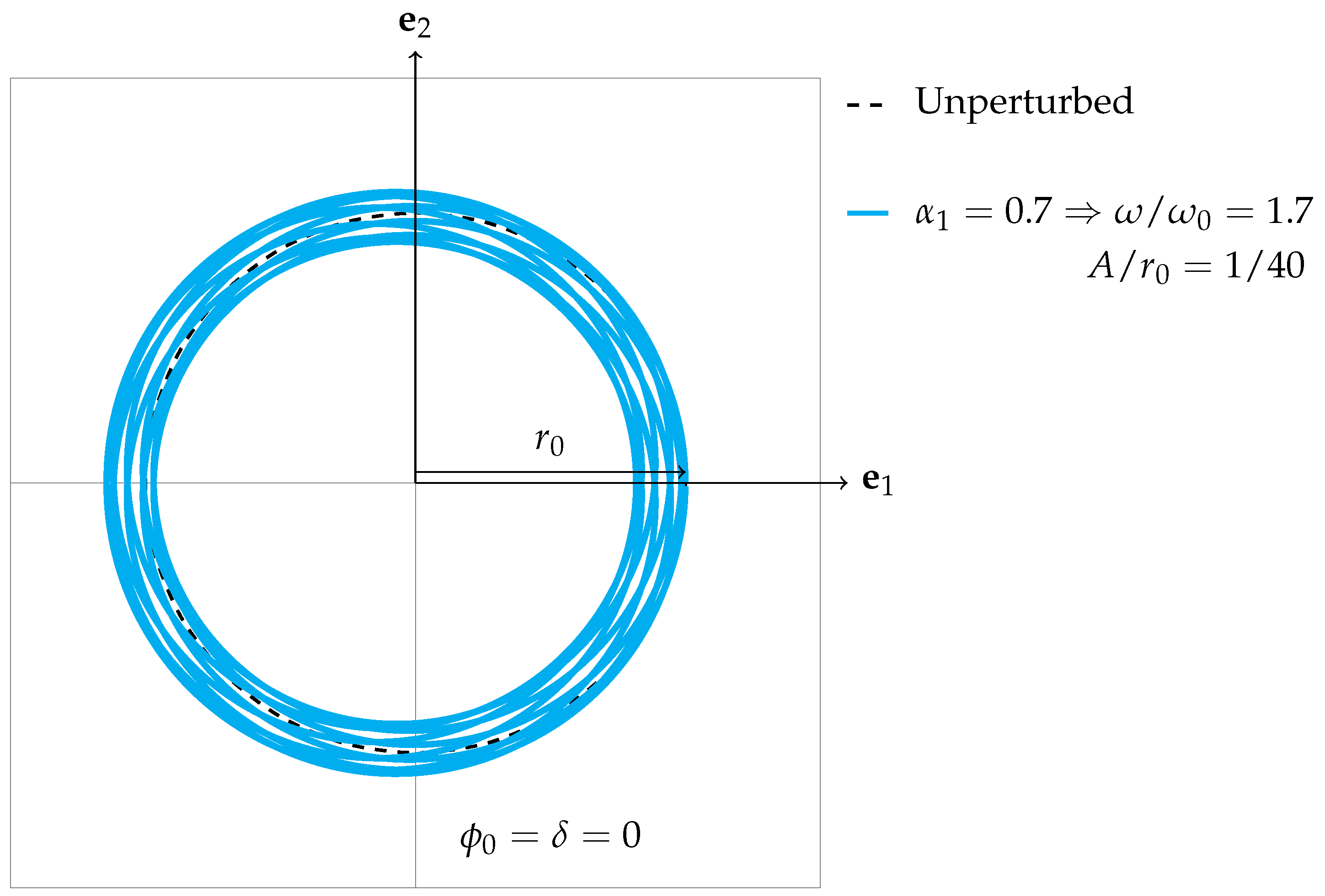
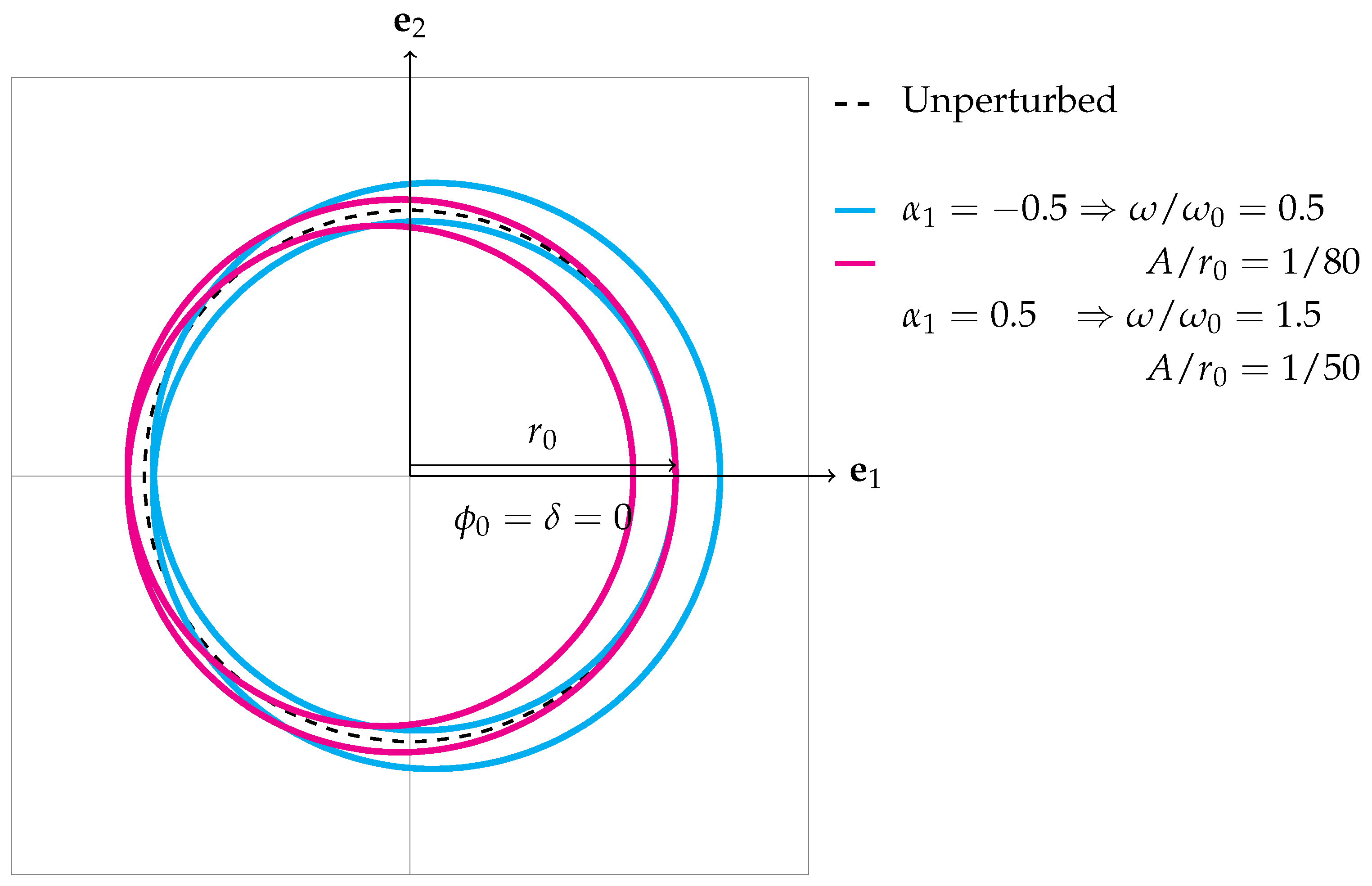
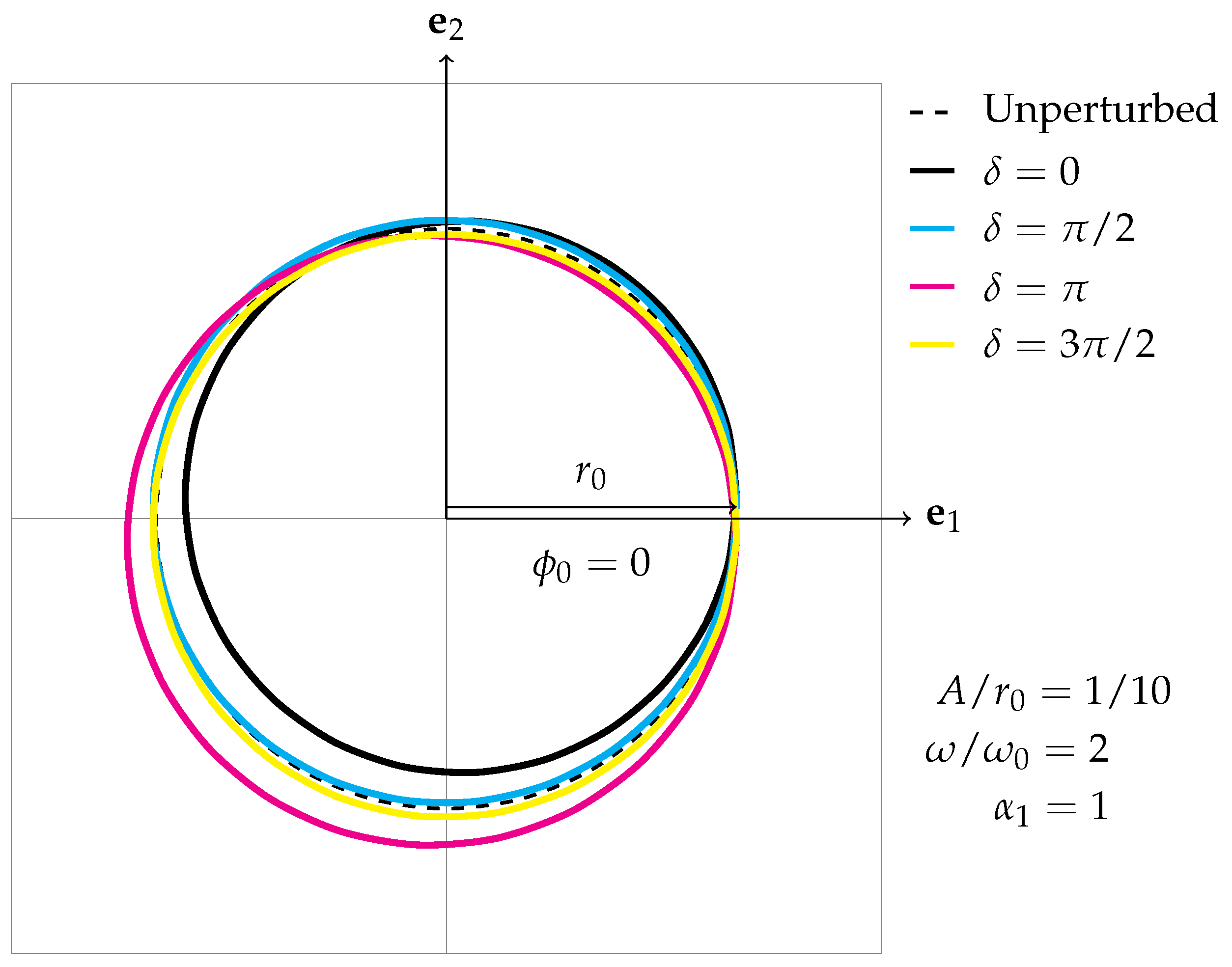
• Figure 2 for ${\alpha }_1=0.7$ (or $\alpha =1.7$) with $A/r_0=1/40$.
• Figure 3 for ${\alpha }_1=\{-0.5,0.5\}$ (or $\alpha =\{0.5,1.5\}$) with $A/r_0=\{1/10,1/4\}$.
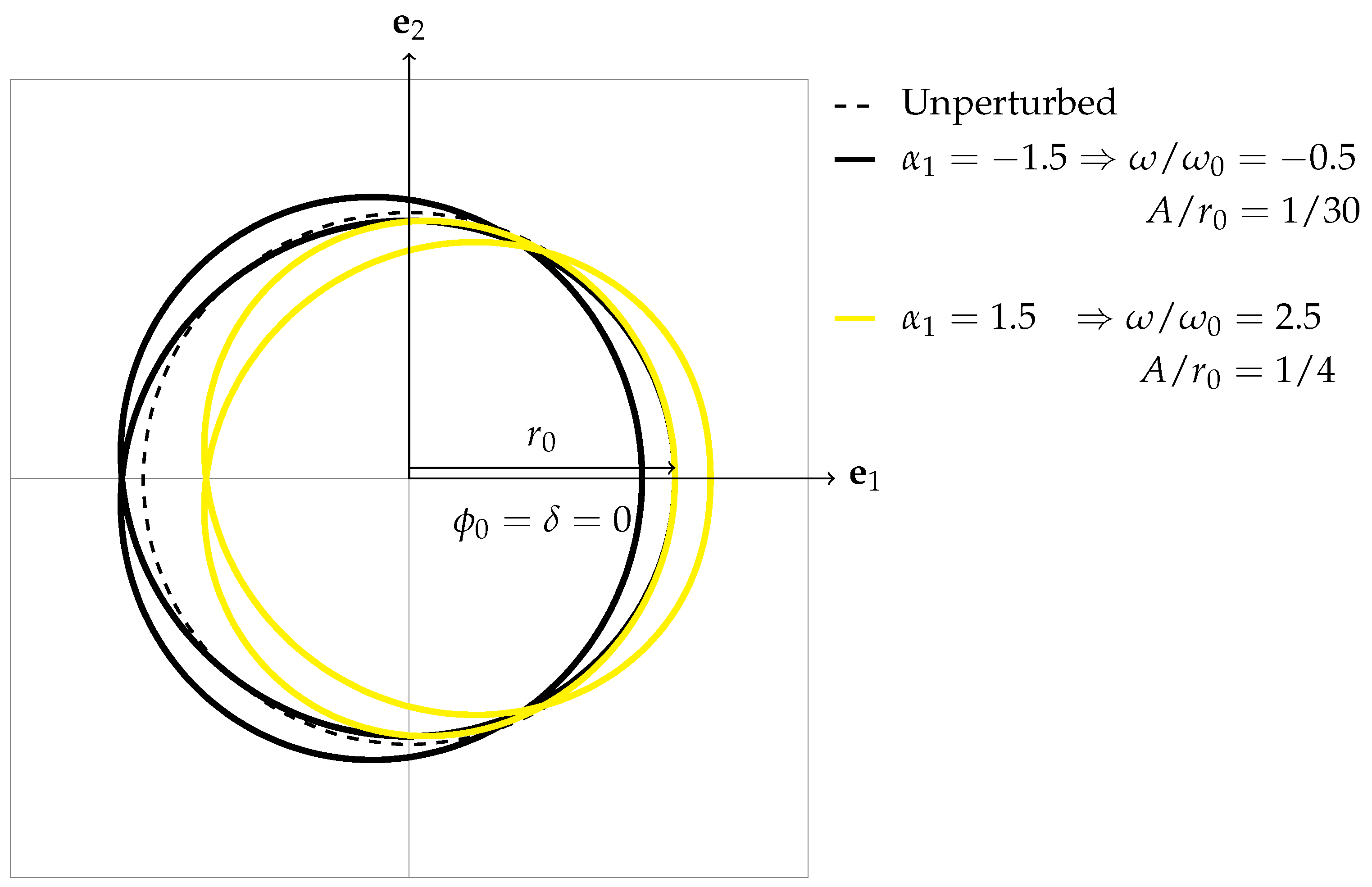
• Figure 4 for ${\alpha }_1=\{-1.5,1.5\}$ (or $\alpha =\{-0.5,2.5\}$) with $A/r_0=\{1/30,1/4\}$.
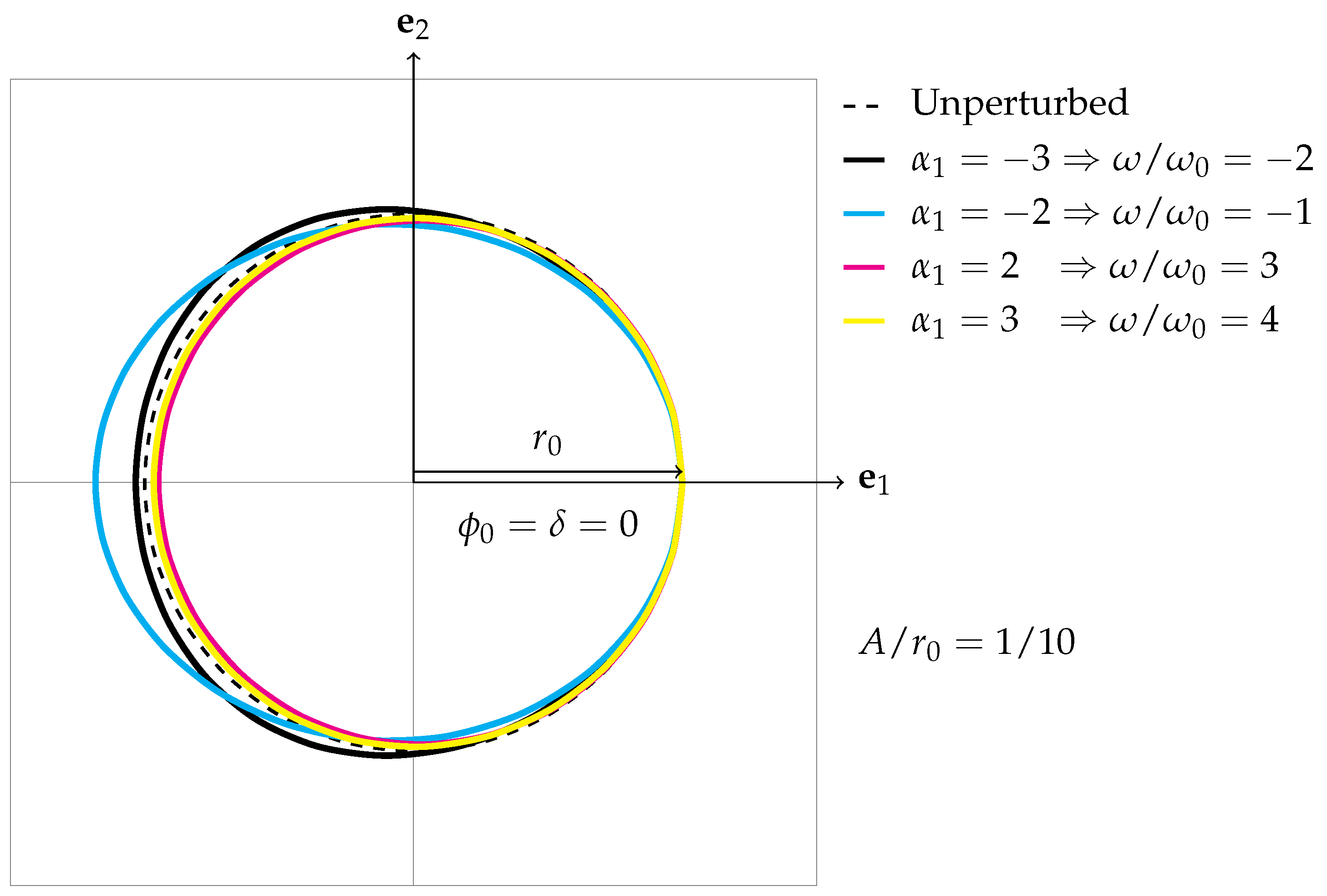
• Figure 5 for ${\alpha }_1=\{-3,-2,2,3\}$ (or $\alpha =\{-2,-1,3,4\}$) with $A/r_0=1/10$.

Note that we chose the values of the light-to-atom force magnitude ratio $A/r_0$ to be small enough ($A/r_0\ll 1$) for the linear perturbation assumption $\mathbf{r}={\mathbf{r}}_0+\lambda {\mathbf{r}}_1$ in Equation (37), but large enough ($A/r_0\approx 1$) so that the shape of the orbit can be seen.

4.6. Electron Orbit at Zeroth Harmonic Resonant Frequency

At displaced frequency ratio ${\alpha }_1=-1$ (which is equivalent to $\alpha =\omega /{\omega }_0=0$), the expression for the position $\mathbf{r}$ in Equation (112) becomes

$$\mathbf{r}={\mathbf{e}}_1\left[{\widehat{c}}_{-1}^{\prime }+({\widehat{r}}_0+{\widehat{c}}_0^{\prime }){\widehat{\psi }}_0+{\widehat{c}}_1^{\prime }{\widehat{\psi }}_0^2\right],$$

(123)

where

$$\begin{array}{cc}\hfill {\widehat{c}}_{-1}^{\prime }& \equiv {\widehat{c}}_{-1}+{\widehat{b}}_1,\hfill \end{array}$$

(124a)

$$\begin{array}{cc}\hfill {\widehat{c}}_0^{\prime }& \equiv {\widehat{c}}_0,\hfill \end{array}$$

(124b)

$$\begin{array}{cc}\hfill {\widehat{c}}_1^{\prime }& \equiv {\widehat{c}}_1+{\widehat{b}}_{-1}\hfill \end{array}$$

(124c)

and

$$\begin{array}{cc}\hfill {\widehat{c}}_{-1}+{\widehat{b}}_1& ={\displaystyle \frac{A}{{\alpha }_1^2({\alpha }_1^2-1)}}\left[-{\displaystyle \frac{3}{8}}({\alpha }_1^3-2{\alpha }_1^2-3{\alpha }_1)e^{(2{\varphi }_0-\delta )\widehat{\mathsf{ı}}}+{\displaystyle \frac{1}{8}}(9{\alpha }_1^3-10{\alpha }_1^2-7{\alpha }_1+12)e^{\widehat{\mathsf{ı}}\delta }\right],\hfill \end{array}$$

(125a)

$$\begin{array}{cc}\hfill {\widehat{c}}_0& ={\displaystyle \frac{A}{{\alpha }_1^2({\alpha }_1^2-1)}}\left[{\displaystyle \frac{6}{8}}({\alpha }_1^3-2{\alpha }_1^2-{\alpha }_1+2)e^{(2{\varphi }_0-\delta )\widehat{\mathsf{ı}}}-{\displaystyle \frac{2}{8}}(5{\alpha }_1^3-6{\alpha }_1^2-5{\alpha }_1+6)e^{\widehat{\mathsf{ı}}\delta }\right],\hfill \end{array}$$

(125b)

$$\begin{array}{cc}\hfill {\widehat{c}}_1+{\widehat{b}}_{-1}& ={\displaystyle \frac{A}{{\alpha }_1^2({\alpha }_1^2-1)}}\left[-{\displaystyle \frac{3}{8}}({\alpha }_1^3-2{\alpha }_1^2+{\alpha }_1+4)e^{(2{\varphi }_0-\delta )\widehat{\mathsf{ı}}}+{\displaystyle \frac{1}{8}}({\alpha }_1^3-2{\alpha }_1^2-3{\alpha }_1)e^{\widehat{\mathsf{ı}}\delta }\right].\hfill \end{array}$$

(125c)

Canceling out ${\alpha }_1+1$ from the numerators and the denominators of the coefficients, we get

$$\begin{array}{cc}\hfill {\widehat{c}}_{-1}+{\widehat{b}}_1\equiv {\widehat{c}}_{-1}^{\prime }& ={\displaystyle \frac{A}{{\alpha }_1^2({\alpha }_1-1)}}\left[-{\displaystyle \frac{3}{8}}({\alpha }_1^2-3{\alpha }_1)e^{(2{\varphi }_0-\delta )\widehat{\mathsf{ı}}}+{\displaystyle \frac{1}{8}}(9{\alpha }_1^2-19{\alpha }_1+12)e^{\widehat{\mathsf{ı}}\delta }\right],\hfill \end{array}$$

(126a)

$$\begin{array}{cc}\hfill {\widehat{c}}_0\equiv {\widehat{c}}_0^{\prime }& ={\displaystyle \frac{A}{{\alpha }_1^2({\alpha }_1-1)}}\left[{\displaystyle \frac{6}{8}}({\alpha }_1^2-3{\alpha }_1+2)e^{(2{\varphi }_0-\delta )\widehat{\mathsf{ı}}}+{\displaystyle \frac{2}{8}}(-5{\alpha }_1^2+11{\alpha }_1-6)e^{\widehat{\mathsf{ı}}\delta }\right],\hfill \end{array}$$

(126b)

$$\begin{array}{cc}\hfill {\widehat{c}}_1+{\widehat{b}}_{-1}\equiv {\widehat{c}}_1^{\prime }& ={\displaystyle \frac{A}{{\alpha }_1^2({\alpha }_1-1)}}\left[-{\displaystyle \frac{3}{8}}({\alpha }_1^2-3{\alpha }_1+4)e^{(2{\varphi }_0-\delta )\widehat{\mathsf{ı}}}+{\displaystyle \frac{1}{8}}({\alpha }_1^2-3{\alpha }_1)e^{\widehat{\mathsf{ı}}\delta }\right].\hfill \end{array}$$

(126c)

This allows us to remove the discontinuity at ${\alpha }_1=-1$, so that we can evaluate the limits of the coefficients as ${\alpha }_1$ approaches $-1$:

$$\begin{array}{cc}\hfill \underset{{\alpha }_1\to -1}{lim}({\widehat{c}}_{-1}+{\widehat{b}}_1)\equiv \underset{{\alpha }_1\to -1}{lim}{\widehat{c}}_{-1}^{\prime }& ={\displaystyle \frac{3}{4}}A{e}^{(2{\varphi }_0-\delta )\widehat{\mathsf{ı}}}-{\displaystyle \frac{5}{2}}A{e}^{\widehat{\mathsf{ı}}\delta },\hfill \end{array}$$

(127a)

$$\begin{array}{cc}\hfill \underset{{\alpha }_1\to -1}{lim}{\widehat{c}}_0\equiv \underset{{\alpha }_1\to -1}{lim}{\widehat{c}}_0^{\prime }& =-{\displaystyle \frac{9}{4}}A{e}^{(2{\varphi }_0-\delta )\widehat{\mathsf{ı}}}+{\displaystyle \frac{11}{4}}A{e}^{\widehat{\mathsf{ı}}\delta },\hfill \end{array}$$

(127b)

$$\begin{array}{cc}\hfill \underset{{\alpha }_1\to -1}{lim}({\widehat{c}}_1+{\widehat{b}}_{-1})\equiv \underset{{\alpha }_1\to -1}{lim}{\widehat{c}}_1^{\prime }& ={\displaystyle \frac{3}{2}}A{e}^{(2{\varphi }_0-\delta )\widehat{\mathsf{ı}}}-{\displaystyle \frac{1}{4}}A{e}^{\widehat{\mathsf{ı}}\delta }.\hfill \end{array}$$

(127c)

Comparing these with the coefficient definitions in Equation (113a–e), we obtain

$$\begin{array}{cc}\hfill c_{-1\rho }^{\prime }& ={\displaystyle \frac{3}{4}}A=0.750A,\hfill \end{array}$$

(128a)

$$\begin{array}{cc}\hfill c_{-1\delta }^{\prime }& =-{\displaystyle \frac{5}{2}}A=-2.500A,\hfill \end{array}$$

(128b)

$$\begin{array}{cc}\hfill c_{0\rho }^{\prime }& =-{\displaystyle \frac{9}{4}}A=-2.250A,\hfill \end{array}$$

(128c)

$$\begin{array}{cc}\hfill c_{0\delta }^{\prime }& ={\displaystyle \frac{11}{4}}A=2.750A,\hfill \end{array}$$

(128d)

$$\begin{array}{cc}\hfill c_{1\rho }^{\prime }& ={\displaystyle \frac{3}{2}}A=1.500A,\hfill \end{array}$$

(128e)

$$\begin{array}{cc}\hfill c_{1\delta }^{\prime }& =-{\displaystyle \frac{1}{4}}=-0.250A,\hfill \end{array}$$

(128f)

$$\begin{array}{cc}\hfill b_{-1\rho }^{\prime }& =0,\hfill \end{array}$$

(128g)

$$\begin{array}{cc}\hfill b_{1\delta }^{\prime }& =0.\hfill \end{array}$$

(128h)

We may substitute these expressions for the coefficient components into the expressions for the x and y components of the position in Equation (115a,b). Since this position is for ${\alpha }_1=-1$ (equivalent to $\alpha =\omega /{\omega }_0=0$), then the corresponding electron’s orbit is still nearly Keplerian, which is approximated by the sum of the Copernican Fourier elements: the eccentric ${\widehat{c}}_{-1}$, deferent ${\widehat{c}}_0^{\prime }{\widehat{\psi }}_0$, and epicycle ${\widehat{c}}_1^{\prime }{\widehat{\psi }}_0^2$ (see Figure 6).

4.7. Electron Ionization at the First Harmonic Resonant Frequency

At displaced frequency ratio ${\alpha }_1=0$ (which is equivalent to $\alpha =\omega /{\omega }_0=1$), the expression for the position $\mathbf{r}$ in Equation (112) becomes

$$\mathbf{r}={\mathbf{e}}_1\left[{\widehat{c}}_{-1}^{\prime }+({\widehat{r}}_0+{\widehat{c}}_0^{\prime }){\widehat{\psi }}_0+{\widehat{c}}_1^{\prime }{\widehat{\psi }}_0^2\right],$$

(129)

where

$$\begin{array}{cc}\hfill {\widehat{c}}_{-1}^{\prime }& \equiv {\widehat{c}}_{-1},\hfill \end{array}$$

(130a)

$$\begin{array}{cc}\hfill {\widehat{c}}_0^{\prime }& \equiv {\widehat{c}}_0+{\widehat{b}}_{-1}+{\widehat{b}}_1,\hfill \end{array}$$

(130b)

$$\begin{array}{cc}\hfill {\widehat{c}}_1^{\prime }& \equiv {\widehat{c}}_1,\hfill \end{array}$$

(130c)

and

$$\begin{array}{cc}\hfill {\widehat{c}}_{-1}& ={\displaystyle \frac{A}{{\alpha }_1^2({\alpha }_1^2-1)}}\left[-{\displaystyle \frac{3}{8}}({\alpha }_1^3-2{\alpha }_1^2-3{\alpha }_1)e^{(2{\varphi }_0-\delta )\widehat{\mathsf{ı}}}+{\displaystyle \frac{9}{8}}({\alpha }_1^3-2{\alpha }_1^2+{\alpha }_1)e^{\widehat{\mathsf{ı}}\delta }\right],\hfill \end{array}$$

(131a)

$$\begin{array}{cc}\hfill {\widehat{c}}_0+{\widehat{b}}_{-1}+{\widehat{b}}_1& ={\displaystyle \frac{A}{{\alpha }_1^2({\alpha }_1^2-1)}}\left[{\displaystyle \frac{6}{8}}({\alpha }_1^3-2{\alpha }_1^2-{\alpha }_1)e^{(2{\varphi }_0-\delta )\widehat{\mathsf{ı}}}+{\displaystyle \frac{2}{8}}(-5{\alpha }_1^3+10{\alpha }_1^2-3{\alpha }_1)e^{\widehat{\mathsf{ı}}\delta }\right],\hfill \end{array}$$

(131b)

$$\begin{array}{cc}\hfill {\widehat{c}}_1& ={\displaystyle \frac{A}{{\alpha }_1^2({\alpha }_1^2-1)}}\left[-{\displaystyle \frac{3}{8}}({\alpha }_1^3-2{\alpha }_1^2+{\alpha }_1)e^{(2{\varphi }_0-\delta )\widehat{\mathsf{ı}}}+{\displaystyle \frac{1}{8}}({\alpha }_1^3-2{\alpha }_1^2-3{\alpha }_1)e^{\widehat{\mathsf{ı}}\delta }\right].\hfill \end{array}$$

(131c)

Since only ${\alpha }_1$ can be factored out from the numerator and not ${\alpha }_1^2$, then an ${\alpha }_1$ factor remains in the denominator, so that in the limit as ${\alpha }_1\to 0$, the coefficients become infinite:

$$\underset{{\alpha }_1\to 0}{lim}|{\widehat{c}}_{-1}^{\prime }|=\underset{{\alpha }_1\to 0}{lim}|{\widehat{c}}_0^{\prime }|=\underset{{\alpha }_1\to 0}{lim}|{\widehat{c}}_1^{\prime }|=\infty .$$

(132)

This makes the position $\mathbf{r}$ also infinite:

$$\underset{{\alpha }_1\to 0}{lim}\left|\mathbf{r}\right|=\infty .$$

(133)

That is, the atom will become ionized as ${\alpha }_1=\omega /{\omega }_0-1\to 0$, which is when the light frequency $\omega$ is equal to the electron’s unperturbed orbital frequency ${\omega }_0$ (see Figure 7 and Figure 8 for the nearly Keplerian electron orbits at ${\alpha }_1=\{-0.01,0.01\}$).

4.8. Electron Orbit at Second Harmonic Resonant Frequency

At displaced frequency ratio ${\alpha }_1=1$ (which is equivalent to $\alpha =\omega /{\omega }_0=2$), the expression for the position $\mathbf{r}$ in Equation (112) becomes

$$\mathbf{r}={\mathbf{e}}_1\left[{\widehat{c}}_{-1}^{\prime }+({\widehat{r}}_0+{\widehat{c}}_0){\widehat{\psi }}_0+{\widehat{c}}_1^{\prime }{\widehat{\psi }}_0^2\right],$$

(134)

where

$$\begin{array}{cc}\hfill {\widehat{c}}_{-1}^{\prime }& \equiv {\widehat{c}}_{-1}+{\widehat{b}}_{-1},\hfill \end{array}$$

(135a)

$$\begin{array}{cc}\hfill {\widehat{c}}_0^{\prime }& \equiv {\widehat{c}}_0,\hfill \end{array}$$

(135b)

$$\begin{array}{cc}\hfill {\widehat{c}}_1^{\prime }& \equiv {\widehat{c}}_1+{\widehat{b}}_1,\hfill \end{array}$$

(135c)

and

$$\begin{array}{cc}\hfill {\widehat{c}}_{-1}+{\widehat{b}}_{-1}& ={\displaystyle \frac{A}{{\alpha }_1^2({\alpha }_1^2-1)}}\left[-{\displaystyle \frac{3}{8}}({\alpha }_1^3-2{\alpha }_1^2-3{\alpha }_1+4)e^{(2{\varphi }_0-\delta )\widehat{\mathsf{ı}}}+{\displaystyle \frac{9}{8}}({\alpha }_1^3-2{\alpha }_1^2+{\alpha }_1)e^{\widehat{\mathsf{ı}}\delta }\right],\hfill \end{array}$$

(136a)

$$\begin{array}{cc}\hfill {\widehat{c}}_0& ={\displaystyle \frac{A}{{\alpha }_1^2({\alpha }_1^2-1)}}\left[{\displaystyle \frac{6}{8}}({\alpha }_1^3-2{\alpha }_1^2-{\alpha }_1+2)e^{(2{\varphi }_0-\delta )\widehat{\mathsf{ı}}}-{\displaystyle \frac{2}{8}}(5{\alpha }_1^3-6{\alpha }_1^2-5{\alpha }_1+6)e^{\widehat{\mathsf{ı}}\delta }\right],\hfill \end{array}$$

(136b)

$$\begin{array}{cc}\hfill {\widehat{c}}_1+{\widehat{b}}_1& ={\displaystyle \frac{A}{{\alpha }_1^2({\alpha }_1^2-1)}}\left[-{\displaystyle \frac{3}{8}}({\alpha }_1^3-2{\alpha }_1^2+{\alpha }_1)e^{(2{\varphi }_0-\delta )\widehat{\mathsf{ı}}}+{\displaystyle \frac{1}{8}}({\alpha }_1^3+6{\alpha }_1^2-19{\alpha }_1+12)e^{\widehat{\mathsf{ı}}\delta }\right].\hfill \end{array}$$

(136c)

Canceling out ${\alpha }_1-1$ from the numerators and the denominators of the ${\widehat{c}}_{-1}^{\prime }$, ${\widehat{c}}_0^{\prime }$, and ${\widehat{c}}_1^{\prime }$ coefficients, we get

$$\begin{array}{cc}\hfill {\widehat{c}}_{-1}+{\widehat{b}}_{-1}\equiv {\widehat{c}}_{-1}^{\prime }& ={\displaystyle \frac{A}{{\alpha }_1^2({\alpha }_1+1)}}\left[-{\displaystyle \frac{3}{8}}({\alpha }_1^2-{\alpha }_1-4)e^{(2{\varphi }_0-\delta )\widehat{\mathsf{ı}}}+{\displaystyle \frac{9}{8}}({\alpha }_1^2-{\alpha }_1)e^{\widehat{\mathsf{ı}}\delta }\right],\hfill \end{array}$$

(137a)

$$\begin{array}{cc}\hfill {\widehat{c}}_0\equiv {\widehat{c}}_0^{\prime }& ={\displaystyle \frac{A}{{\alpha }_1^2({\alpha }_1+1)}}\left[{\displaystyle \frac{3}{4}}({\alpha }_1^2-{\alpha }_1-2)e^{(2{\varphi }_0-\delta )\widehat{\mathsf{ı}}}-{\displaystyle \frac{1}{4}}(5{\alpha }_1^2-{\alpha }_1-6)e^{\widehat{\mathsf{ı}}\delta }\right],\hfill \end{array}$$

(137b)

$$\begin{array}{cc}\hfill {\widehat{c}}_1+{\widehat{b}}_1\equiv {\widehat{c}}_1^{\prime }& ={\displaystyle \frac{A}{{\alpha }_1^2({\alpha }_1+1)}}\left[-{\displaystyle \frac{3}{8}}({\alpha }_1^2-{\alpha }_1)e^{(2{\varphi }_0-\delta )\widehat{\mathsf{ı}}}+{\displaystyle \frac{1}{8}}({\alpha }_1^2+7{\alpha }_1-12)e^{\widehat{\mathsf{ı}}\delta }\right].\hfill \end{array}$$

(137c)

This allows us to remove the discontinuity at ${\alpha }_1=1$, so that we can evaluate the limits of the coefficients as ${\alpha }_1$ approaches 1:

$$\begin{array}{cc}\hfill \underset{{\alpha }_1\to 1}{lim}({\widehat{c}}_{-1}+{\widehat{b}}_{-1})\equiv \underset{{\alpha }_1\to 1}{lim}{\widehat{c}}_{-1}^{\prime }& =A\left[{\displaystyle \frac{3}{4}}{e}^{(2{\varphi }_0-\delta )\widehat{\mathsf{ı}}}\right],\hfill \end{array}$$

(138a)

$$\begin{array}{cc}\hfill \underset{{\alpha }_1\to 1}{lim}{\widehat{c}}_0\equiv \underset{{\alpha }_1\to 1}{lim}{\widehat{c}}_0^{\prime }& =A\left[-{\displaystyle \frac{3}{4}}{e}^{(2{\varphi }_0-\delta )\widehat{\mathsf{ı}}}+{\displaystyle \frac{1}{4}}{e}^{\widehat{\mathsf{ı}}\delta }\right],\hfill \end{array}$$

(138b)

$$\begin{array}{cc}\hfill \underset{{\alpha }_1\to 1}{lim}({\widehat{c}}_1+{\widehat{b}}_1)\equiv \underset{{\alpha }_1\to 1}{lim}{\widehat{c}}_1^{\prime }& =A\left[-{\displaystyle \frac{1}{4}}{e}^{\widehat{\mathsf{ı}}\delta }\right].\hfill \end{array}$$

(138c)

Comparing these with the coefficient definitions in Equation (113a–e), we obtain

$$\begin{array}{cc}\hfill c_{-1\rho }^{\prime }& ={\displaystyle \frac{3}{4}}A=0.750A,\hfill \end{array}$$

(139a)

$$\begin{array}{cc}\hfill c_{-1\delta }^{\prime }& =0,\hfill \end{array}$$

(139b)

$$\begin{array}{cc}\hfill c_{0\rho }^{\prime }& =-{\displaystyle \frac{3}{4}}A=-0.750A,\hfill \end{array}$$

(139c)

$$\begin{array}{cc}\hfill c_{0\delta }^{\prime }& ={\displaystyle \frac{1}{4}}A=0.250A,\hfill \end{array}$$

(139d)

$$\begin{array}{cc}\hfill c_{1\rho }^{\prime }& =0,\hfill \end{array}$$

(139e)

$$\begin{array}{cc}\hfill c_{1\delta }^{\prime }& =-{\displaystyle \frac{1}{4}}A=-0.250A,\hfill \end{array}$$

(139f)

$$\begin{array}{cc}\hfill b_{-1\rho }^{\prime }& =0,\hfill \end{array}$$

(139g)

$$\begin{array}{cc}\hfill b_{1\delta }^{\prime }& =0.\hfill \end{array}$$

(139h)

We may substitute these expressions for the coefficient components into the expressions for the x and y components of the position in Equation (115a,b). Since this position is for ${\alpha }_1=\omega /{\omega }_0-1=1$ (equivalent to $\omega =2{\omega }_0$), then the corresponding electron’s orbit is still nearly Keplerian, which is approximated by the sum of the Copernican Fourier elements: the eccentric ${\widehat{c}}_{-1}$, the deferent ${\widehat{c}}_0^{\prime }{\widehat{\psi }}_0$, and the epicycle ${\widehat{c}}_1^{\prime }{\widehat{\psi }}_0^2$ (see Figure 9).

4.9. Electron Orbits: Frequency Conversion and Harmonic Generation

We assumed that before time $t=0$, a hydrogen electron of charge $-q$ is in a counterclockwise circular orbit around the proton of charge q at the origin of a coordinate system spanned by orthonormal vectors ${\mathbf{e}}_1$ and ${\mathbf{e}}_2$. The position $\mathbf{r}$ of the electron with respect to the proton is given by Equation (27):

$$\mathbf{r}={\mathbf{e}}_1{\widehat{r}}_0{\widehat{\psi }}_0={\mathbf{e}}_1{r}_0{e}^{\widehat{\mathsf{ı}}({\omega }_{0}t+{\varphi }_0)},$$

(140)

where $r_0$ is the electron’s orbital radius, ${\omega }_0$ is the electron’s orbital angular frequency, and ${\varphi }_0$ is the orbital phase. Note that ${\widehat{r}}_0=r_0{e}^{\widehat{\mathsf{ı}}{\varphi }_0}$ is the electron’s complex initial position and ${\widehat{\psi }}_0=e^{\widehat{\mathsf{ı}}{\omega }_{0}t}$ is the electron’s unperturbed orbital wave function that acts as a counterclockwise circular rotation operator.

We also assumed that at time $t\ge 0$, the circularly polarized light is switched on. The light’s electric field $\mathbf{E}$ is given by Equation (22), which we may rewrite as

$$\mathbf{E}={\mathbf{e}}_1\widehat{a}\widehat{\psi }={\mathbf{e}}_1\widehat{a}{\widehat{\psi }}_0^{\alpha }={\mathbf{e}}_{1}a{\widehat{\psi }}_0^{({\alpha }_1+1)}={\mathbf{e}}_{1}a{e}^{\widehat{\mathsf{ı}}(\omega t+\delta )},$$

(141)

where $\alpha =\omega /{\omega }_0$ is the light-to-atom frequency ratio, ${\alpha }_1=\alpha -1$ is the displaced light-to-atom frequency ratio, $a=|\widehat{a}|$ is the electric field amplitude, $\omega$ is the rotational angular frequency, and $\delta$ is the rotational phase. If $\omega >0$, the light is left-circularly polarized (rotating counterclockwise). If $\omega <0$, the light is right-circularly polarized (rotating clockwise). And if $\omega =0$, the electric field is constant (c.f., DC Stark Effect).

In response to this switching on of the circularly polarized radiation at time $t\ge 0$, the atom changes its orbit. But unlike in the Bohr model, the atom does not suddenly jump to a new circular orbit with a different radius. Instead, the electron starts at its unperturbed state at time $t=0$, so that initial position and velocity of the electron at its new orbit are the same as its final position and velocity at its unperturbed orbit, as given in Equations (101a,b) and (103a,b):

$$\begin{array}{cc}\hfill \mathbf{r}\left(0^{-}\right)=\mathbf{r}\left(0^{+}\right)& ={\mathbf{e}}_1{\widehat{r}}_0={\mathbf{e}}_1{r}_0{e}^{\widehat{\mathsf{ı}}{\varphi }_0},\hfill \end{array}$$

(142a)

$$\begin{array}{cc}\hfill \dot{\mathbf{r}}\left(0^{-}\right)=\dot{\mathbf{r}}\left(0^{+}\right)& ={\mathbf{e}}_1\widehat{\mathsf{ı}}{\omega }_0{\widehat{r}}_0={\mathbf{e}}_2{\omega }_0{r}_0{e}^{\widehat{\mathsf{ı}}{\varphi }_0}.\hfill \end{array}$$

(142b)

The new orbit of the electron is given by Equation (112)

$$\mathbf{r}={\mathbf{e}}_1\left[{\widehat{c}}_{-1}+({\widehat{r}}_0+{\widehat{c}}_0){\widehat{\psi }}_0+{\widehat{c}}_1{\widehat{\psi }}_0^2+{\widehat{b}}_{-1}{\widehat{\psi }}_0^{-({\alpha }_1-1)}+{\widehat{b}}_1{\widehat{\psi }}_0^{({\alpha }_1+1)}\right].$$

(143)

where the $\widehat{c}$ and $\widehat{b}$ coefficients of the orbital wave functions are given in Equations (113a) to (114h). The values of these coefficients as a function of ${\alpha }_1=\alpha -1$ are given in

Table 1. The decomposition of the $\widehat{c}$ and $\widehat{b}$ coefficients as a linear combination of the phase exponential functions $e^{(2{\varphi }_0-\delta )\widehat{\mathsf{ı}}}$ and $e^{\widehat{\mathsf{ı}}\delta }$ for the displaced frequency ratio ${\alpha }_1\in [-5,5]$, with ${\alpha }_1\ne \{-1,0,1\}$. The subscript $\rho$ refers to the component along $e^{(2{\varphi }_0-\delta )\widehat{\mathsf{ı}}}$, while the subscript $\delta$ refers to the component along $e^{\widehat{\mathsf{ı}}\delta }$. The bar over the c or b component means that the component is normalized with respect to the normalized light amplitude $A=q|\widehat{a}|/m{\omega }_0^2$. For example, ${\overline{c}}_{1\rho }=c_{1\rho }/A$. Note that ${\alpha }_1=\omega /{\omega }_0-1$ is the displaced light-to-atom frequency ratio.

${\mathit{\alpha }}_1$	${\overline{\mathit{c}}}_{-1\mathit{\rho }}$	${\overline{\mathit{c}}}_{-1\mathit{\delta }}$	${\overline{\mathit{c}}}_{0\mathit{\rho }}$	${\overline{\mathit{c}}}_{0\mathit{\delta }}$	${\overline{\mathit{c}}}_{1\mathit{\rho }}$	${\overline{\mathit{c}}}_{1\mathit{\delta }}$	${\overline{\mathit{b}}}_{-1\mathit{\rho }}$	${\overline{\mathit{b}}}_{1\mathit{\delta }}$
−5.0	0.100	−0.338	−0.210	0.310	0.113	−0.033	−0.003	0.061
−4.0	0.131	−0.469	−0.281	0.406	0.156	−0.044	−0.006	0.106
−3.0	0.188	−0.750	−0.417	0.583	0.250	−0.063	−0.021	0.229
−2.0	0.313	−1.688	−0.750	1.000	0.563	−0.104	−0.125	0.792
−1.9	0.333	−1.908	−0.810	1.073	0.636	−0.111	−0.159	0.946
−1.8	0.357	−2.188	−0.880	1.157	0.729	−0.119	−0.207	1.149
−1.7	0.384	−2.553	−0.960	1.254	0.851	−0.128	−0.275	1.426
−1.6	0.415	−3.047	−1.055	1.367	1.016	−0.138	−0.376	1.818
−1.5	0.450	−3.750	−1.167	1.500	1.250	−0.150	−0.533	2.400
−1.4	0.491	−4.821	−1.301	1.658	1.607	−0.164	−0.797	3.327
−1.3	0.539	−6.635	−1.464	1.849	2.212	−0.180	−1.286	4.965
−1.2	0.597	−10.313	−1.667	2.083	3.438	−0.199	−2.367	8.428
−1.1	0.666	−21.477	−1.921	2.376	7.159	−0.222	−5.903	19.323
−1.0
−0.9	0.855	23.750	−2.685	3.241	−7.917	−0.285	9.747	−26.706
−0.8	0.990	12.656	−3.281	3.906	−4.219	−0.330	6.510	−16.233
−0.7	1.166	9.107	−4.133	4.847	−3.036	−0.389	6.002	−13.565
−0.6	1.406	7.500	−5.417	6.250	−2.500	−0.469	6.510	−13.281
−0.5	1.750	6.750	−7.500	8.500	−2.250	−0.583	8.000	−14.667
−0.4	2.277	6.563	−11.250	12.500	−2.188	−0.759	11.161	−18.304
−0.3	3.173	6.964	−19.167	20.833	−2.321	−1.058	18.315	−26.740
−0.2	5.000	8.438	−41.250	43.750	−2.813	−1.667	39.063	−50.521
−0.1	10.568	13.750	−157.500	162.500	−4.583	−3.523	151.515	−172.727
0.0
0.1	−12.083	−9.205	−142.500	137.500	3.068	4.028	151.515	−132.323
0.2	−6.562	−3.750	−33.750	31.250	1.250	2.187	39.062	−29.687
0.3	−4.821	−2.019	−14.167	12.500	0.673	1.607	18.315	−12.088
0.4	−4.063	−1.205	−7.500	6.250	0.402	1.354	11.161	−6.399
0.5	−3.750	−0.750	−4.500	3.500	0.250	1.250	8.000	−4.000
0.6	−3.750	−0.469	−2.917	2.083	0.156	1.250	6.510	−2.865
0.7	−4.107	−0.284	−1.990	1.276	0.095	1.369	6.002	−2.361
0.8	−5.156	−0.156	−1.406	0.781	0.052	1.719	6.510	−2.344
0.9	−8.750	−0.066	−1.019	0.463	0.022	2.917	9.747	−3.314
1.0
1.1	6.477	0.049	−0.558	0.103	−0.016	−2.159	−5.903	2.007
1.2	2.812	0.085	−0.417	0.000	−0.028	−0.937	−2.367	0.852
1.3	1.635	0.113	−0.311	−0.074	−0.038	−0.545	−1.286	0.506
1.4	1.071	0.134	−0.230	−0.128	−0.045	−0.357	−0.797	0.351
1.5	0.750	0.150	−0.167	−0.167	−0.050	−0.250	−0.533	0.267
1.6	0.547	0.162	−0.117	−0.195	−0.054	−0.182	−0.376	0.215
1.7	0.410	0.172	−0.078	−0.216	−0.057	−0.137	−0.275	0.181
1.8	0.312	0.179	−0.046	−0.231	−0.060	−0.104	−0.207	0.157
1.9	0.241	0.184	−0.021	−0.242	−0.061	−0.080	−0.159	0.139
2.0	0.188	0.188	0.000	−0.250	−0.063	−0.063	−0.125	0.125
3.0	0.000	0.188	0.083	−0.250	−0.063	0.000	−0.021	0.063
4.0	−0.031	0.169	0.094	−0.219	−0.056	0.010	−0.006	0.040
5.0	−0.038	0.150	0.090	−0.190	−0.050	0.013	−0.003	0.028

. Notice that in Equation (143) the coefficients ${\widehat{c}}_{-1}$, ${\widehat{c}}_0$, and ${\widehat{c}}_1$ are for the zeroth, first, and second harmonics of the unperturbed orbital wave function ${\widehat{\psi }}_0=e^{\widehat{\mathsf{ı}}{\omega }_{0}t}$. On the other hand, the coefficient ${\widehat{b}}_1$ is for the wave function ${\widehat{\psi }}_0^{{\alpha }_1+1}$ of circularly polarized light, while the coefficient ${\widehat{b}}_{-1}$ is for the mixed wave function ${\widehat{\psi }}_0^{-({\alpha }_1-1)}$:

$$\begin{array}{cc}\hfill {\widehat{\psi }}_0^{{\alpha }_1+1}& ={\widehat{\psi }}_0^{\alpha }=\widehat{\psi }=e^{\widehat{\mathsf{ı}}\omega t},\hfill \end{array}$$

(144a)

$$\begin{array}{cc}\hfill {\widehat{\psi }}_0^{-({\alpha }_1-1)}& ={\widehat{\psi }}_0^{-(\alpha -2)}=e^{-\widehat{\mathsf{ı}}(\omega -2{\omega }_0)t}.\hfill \end{array}$$

(144b)

Now, the $\widehat{c}$ and $\widehat{b}$ coefficients in Equations (113a) to (114h) have the same denominator:

$${\alpha }_1^2({\alpha }_1^2-1)={(\alpha -1)}^2({(\alpha -1)}^2-1).$$

(145)

This means that the orbit will become resonant at three light-to-atom displaced frequency ratios:

$${\alpha }_1=\alpha -1=\{-1,0,1\},$$

(146)

which is equivalent to the light-to-atom frequency ratio

$$\alpha ={\displaystyle \frac{\omega }{{\omega }_0}}=\{0,1,2\}.$$

(147)

That is, the atom will resonate with the incident circularly polarized light only if the rotational angular frequency of light $\omega$ is the zeroth, first, or second harmonic of the electron’s orbital angular frequency ${\omega }_0$.

We evaluated the position $\mathbf{r}$ of the electron at ${\alpha }_1=\{-1,0,1\}$ (or at $\alpha =\{0,1,2\}$), as given in Equation (123). We showed that the $\widehat{b}$ coefficients become mixed with the $\widehat{c}$ coefficients at these resonant frequencies:

$$\begin{array}{cc}\hfill {\alpha }_1=-1:\mathbf{r}& ={\mathbf{e}}_1\left[({\widehat{c}}_{-1}+{\widehat{b}}_1)+({\widehat{r}}_0+{\widehat{c}}_0){\widehat{\psi }}_0+({\widehat{c}}_1+{\widehat{b}}_{-1}){\widehat{\psi }}_0^2\right],\hfill \end{array}$$

(148a)

$$\begin{array}{cc}\hfill {\alpha }_1=0:\mathbf{r}& ={\mathbf{e}}_1\left[{\widehat{c}}_{-1}+({\widehat{r}}_0+{\widehat{c}}_0+{\widehat{b}}_{-1}+{\widehat{b}}_1){\widehat{\psi }}_0+{\widehat{c}}_1{\widehat{\psi }}_0^2\right],\hfill \end{array}$$

(148b)

$$\begin{array}{cc}\hfill {\alpha }_1=1:\mathbf{r}& ={\mathbf{e}}_1\left[({\widehat{c}}_{-1}+{\widehat{b}}_{-1})+({\widehat{r}}_0+{\widehat{c}}_0){\widehat{\psi }}_0+({\widehat{c}}_1+{\widehat{b}}_1){\widehat{\psi }}_0^2\right].\hfill \end{array}$$

(148c)

We showed that the electron’s orbit becomes discontinuous and divergent at ${\alpha }_1=0$ (or at $\alpha =0$) which may result to ionization. On the other hand, we showed that the electron’s orbit is finite and continuous at ${\alpha }_1=\{-1,1\}$ (or at $\alpha =\{0,1,2\}$). The values of the $\widehat{c}$ and $\widehat{b}$ coefficients near these resonant frequencies are given in

Table 2. The position $\mathbf{r}={\mathbf{e}}_1\left[{\widehat{c}}_{-1}+({\widehat{r}}_0+{\widehat{c}}_0){\widehat{\psi }}_0+{\widehat{c}}_1{\psi }_0^2+{\widehat{b}}_{-1}{\widehat{\psi }}_0^{-({\alpha }_1-1)}+{\widehat{b}}_1{\widehat{\psi }}_0^{({\alpha }_1+1)}\right]$ of the hydrogen electron reduces to $\mathbf{r}={\mathbf{e}}_1({\widehat{c}}_{-1}^{\prime }+({\widehat{r}}_0+{\widehat{c}}_0^{\prime }){\widehat{\psi }}_0+{\widehat{c}}_1^{\prime }{\psi }_0^2)$ in the limit as the light-to-atom displaced frequency ratio ${\alpha }_1=(\alpha -1)\to \{-1,0,1\}$ (or $\alpha =\omega /{\omega }_0\to \{0,1,2\}$). The electron’s unperturbed position is $\mathbf{r}={\mathbf{e}}_1{r}_0{e}^{\widehat{\mathsf{ı}}({\omega }_{0}t+{\varphi }_0)}$, where $r_0=\left|{\widehat{r}}_0\right|$ is the electron’s orbital radius and ${\varphi }_0$ is the electron’s orbital phase. On the other hand, the electric field of the perturbing circularly polarized light is $\mathbf{E}={\mathbf{e}}_1\widehat{a}{\widehat{\psi }}_0^{{\alpha }_1+1}={\mathbf{e}}_1\left|\widehat{a}\right|e^{\widehat{\mathsf{ı}}(\omega t+\delta )}$, where $|\widehat{a}|$ and $\delta$ are the amplitude and phase of light’s electric field. Note that $\widehat{c}=A({\overline{c}}_{\rho }{e}^{\widehat{\mathsf{ı}}\rho }+{\overline{c}}_{\delta }{e}^{\widehat{\mathsf{ı}}\delta })$ and $\widehat{b}=A({\overline{b}}_{\rho }{e}^{\widehat{\mathsf{ı}}\rho }+{\overline{b}}_{\delta }{e}^{\widehat{\mathsf{ı}}\delta })$, where $\rho =2{\varphi }_0-\delta$, $A=q|\widehat{a}|/m{\omega }_0^2$, and ${\overline{b}}_{-1\delta }={\overline{b}}_{1\rho }=0$. Notice that the primed coefficients are continuous and finite as ${\alpha }_1\to \{-1,1\}$ (or $\alpha \to \omega /{\omega }_0=\{0,2\}$), but discontinuous and divergent as ${\alpha }_1\to 0$ (or $\alpha =\omega /{\omega }_0\to 1$).

${\mathit{\alpha }}_1$	${\overline{\mathit{c}}}_{-1\mathit{\rho }}$	${\overline{\mathit{c}}}_{-1\mathit{\delta }}$	${\overline{\mathit{c}}}_{0\mathit{\rho }}$	${\overline{\mathit{c}}}_{0\mathit{\delta }}$	${\overline{\mathit{c}}}_{1\mathit{\rho }}$	${\overline{\mathit{c}}}_{1\mathit{\delta }}$	${\overline{\mathit{b}}}_{-1\mathit{\rho }}$	${\overline{\mathit{b}}}_{1\mathit{\delta }}$
−1.01	0.741	−223.886	−2.213	2.708	74.629	−0.247	−73.156	221.425
−1.00	…	…	…	…	…	…	…	…
−0.99	0.759	226.136	−2.288	2.793	−75.379	−0.253	76.907	−228.676
−0.01	112	115	−15,075	15,125	−38	−37	15,002	−15,203
0.00	…	…	…	…	…	…	…	…
0.01	−113	−110	−14,925	14,875	37	38	15,002	−14,802
0.99	−76.136	−0.006	−0.773	0.268	0.002	25.379	76.907	−25.641
1.00	…	…	…	…	…	…	…	…
1.01	73.886	0.006	−0.728	0.233	−0.002	−24.629	−73.156	24.390
${\mathit{\alpha }}_{\mathbf{1}}$	${\overline{\mathit{c}}}_{\mathbf{-}\mathbf{1}\mathit{\rho }}^{\mathbf{\prime }}$	${\overline{\mathit{c}}}_{\mathbf{-}\mathbf{1}\mathit{\delta }}^{\mathbf{\prime }}$	${\overline{\mathit{c}}}_{\mathbf{0}\mathit{\rho }}^{\mathbf{\prime }}$	${\overline{\mathit{c}}}_{\mathbf{0}\mathit{\delta }}^{\mathbf{\prime }}$	${\overline{\mathit{c}}}_{\mathbf{1}\mathit{\rho }}^{\mathbf{\prime }}$	${\overline{\mathit{c}}}_{\mathbf{1}\mathit{\delta }}^{\mathbf{\prime }}$
−1.01	0.741	−2.461	−2.213	2.708	1.472	−0.247
−1.00	0.750	−2.500	−2.250	2.750	1.500	−0.250
−0.99	0.759	−2.540	−2.288	2.793	1.529	−0.253
−0.01	112	115	−73	−78	−38	−37
0.00	…	…	…	…	…	…
0.01	−113	−110	77	73	37	38
0.99	0.771	−0.006	−0.773	0.268	0.002	−0.262
1.00	0.750	0.000	−0.750	0.250	0.000	−0.250
1.01	0.730	0.006	−0.728	0.233	−0.002	−0.238

.

In order to make the frequency conversion clearer, we may denote the set of orbital frequencies of the position $\mathbf{r}$ in Equation (143) as

$${\mathsf{\Omega }}_{\mathbf{r}}=[0,{\omega }_0,2{\omega }_0;-(\omega -2{\omega }_0),\omega ].$$

(149)

Using this notation, the orbital frequencies of the electron’s unperturbed orbit position ${\mathbf{r}}_0$ and that of the electric field $\mathbf{E}$ of circularly polarized light may be written as

$$\begin{array}{cc}\hfill {\mathsf{\Omega }}_{{\mathbf{r}}_0}& =[,{\omega }_0,;,],\hfill \end{array}$$

(150a)

$$\begin{array}{cc}\hfill {\mathsf{\Omega }}_{\mathbf{E}}& =[,,;,\omega ].\hfill \end{array}$$

(150b)

The light–atom interaction may then be expressed as

$${\mathsf{\Omega }}_{\mathbf{E}}\to {\mathsf{\Omega }}_{{\mathbf{r}}_0}\Rightarrow {\mathsf{\Omega }}_{\mathbf{r}}.$$

(151)

At ${\alpha }_1=\{-1,0,1\}$ (or at light-to-atom frequency ratio $\alpha =\omega /{\omega }_0=\{0,1,2\}$), the frequencies of the orbit of the hydrogen electron are as follows:

$$\begin{array}{cc}\hfill \omega /{\omega }_0=0:{\mathsf{\Omega }}_{\mathbf{r}}& =[0,{\omega }_0,2{\omega }_0;2{\omega }_0,0],\hfill \end{array}$$

(152a)

$$\begin{array}{cc}\hfill \omega /{\omega }_0=1:{\mathsf{\Omega }}_{\mathbf{r}}& =[0,{\omega }_0,2{\omega }_0;{\omega }_0,{\omega }_0],\hfill \end{array}$$

(152b)

$$\begin{array}{cc}\hfill \omega /{\omega }_0=2:{\mathsf{\Omega }}_{\mathbf{r}}& =[0,{\omega }_0,2{\omega }_0;0,2{\omega }_0].\hfill \end{array}$$

(152c)

At light frequency $\omega =0$, the orbit resonates not only at the zeroth harmonic of the electron’s unperturbed orbital angular frequency ${\omega }_0$, but also at the first harmonic (higher harmonic) and second harmonic (higher harmonic) as well. At light frequency $\omega ={\omega }_0$, the orbit resonates not only at the first harmonic, but also at the zeroth (subharmonic) and the second harmonic (higher harmonic) as well. (But the orbit is divergent, so ionization occurs.) And at light frequency $\omega =2{\omega }_0$, the orbit resonates not only at the second harmonic, but also at the zeroth harmonic (subharmonic) and first harmonic (subharmonic) as well. These results agree with numerical simulations of the classical interaction of light with a hydrogen-like atom computed with a realistic effective radial potential and radiation damping force (proportional to the time derivative of acceleration):

…if the laser frequency is below the natural oscillation frequency of the optical electron, then laser interaction produces higher harmonics. In the opposite case, in addition to higher harmonics, the sub-harmonics may occur [57].

5. Light–Atom Interaction: Model Limitations and Proposed Corrections

5.1. Lorentz Oscillator, Refractive Index, and Absorption Coefficient

In the standard Lorentz oscillator model with damping, the hydrogen electron is treated as a mass m attached to a spring with force constant k and damping coefficient $\gamma$. When the complex electric field $E_0{e}^{i\omega t}$ of light hits the atom, the electron’s position will be displaced by $\mathbf{x}$ from its unperturbed position, which satisfies the linear differential equation [56]

$$\ddot{x}+{\displaystyle \frac{\gamma }{m}}\dot{x}+{\omega }_0^{2}x=-{\displaystyle \frac{q}{m}}{E}_0{e}^{i\omega t}.$$

(153)

The solution to this equation is

$${\displaystyle x=\frac{-q/m}{-{\omega }^2+i\frac{\gamma }{m}\omega +{\omega }_0^2}{E}_0{e}^{\widehat{\mathsf{ı}}\omega t}.}$$

(154)

Notice that the displacement x is proportional to the electric field of light $E_0{e}^{i\omega t}$; the complex proportionality constant only changes both the phase and magnitude of light’s electric field, but not its frequency $\omega$. This proportionality allows for the straightforward computation of the permittivity, refractive index, and absorption coefficient of light: at the resonant frequency $\omega ={\omega }_0$, the Lorentz oscillator would have an anomalous dispersion and a peak energy absorption.

In our Coulomb oscillator model, the differential equation for the complex perturbation ${\widehat{r}}_1$ is given in Equation (49), which we may rewrite as

$${\ddot{\widehat{r}}}_1+2\widehat{\mathsf{ı}}{\omega }_0{\dot{\widehat{r}}}_1-{\displaystyle \frac{3}{2}}{\omega }_0^2\left({\widehat{r}}_1+e^{2{\varphi }_0\widehat{\mathsf{ı}}}{\widehat{r}}_1^{\ast }\right)=-{\displaystyle \frac{q}{m}}\widehat{a}{e}^{\widehat{\mathsf{ı}}(\omega -{\omega }_0)t},$$

(155)

where we used the exponential definitions of the wave functions $\widehat{\psi }=e^{\widehat{\mathsf{ı}}\omega t}$ and ${\widehat{\psi }}_0=e^{\widehat{\mathsf{ı}}{\omega }_{0}t}$ in Equations (23b) and (28b). The position $\mathbf{r}$ of the electron we obtained is given in Equation (112), which we may also similarly rewrite as

$$\mathbf{r}={\mathbf{e}}_1\left[{\widehat{c}}_{-1}+({\widehat{r}}_0+{\widehat{c}}_0)e^{\widehat{\mathsf{ı}}{\omega }_{0}t}+{\widehat{c}}_1{e}^{\widehat{\mathsf{ı}}\left(2{\omega }_0\right)t}+{\widehat{b}}_{-1}{e}^{-\widehat{\mathsf{ı}}(\omega -2{\omega }_0)t}+{\widehat{b}}_1{e}^{\widehat{\mathsf{ı}}\omega t}\right].$$

(156)

Notice that the position $\mathbf{r}$ is not proportional to the circularly polarized electric field $\mathbf{E}={\mathbf{e}}_1\widehat{a}{e}^{\widehat{\mathsf{ı}}\omega t}$ of light, since there are five wave functions with at least three different frequencies. This makes the computation of the permittivity, refractive index, and absorption coefficient not as straightforward as in the Lorentz model. Nevertheless, we know that unlike the single light-to-atom resonance frequency ratio in the Lorentz model (i.e., $\omega /{\omega }_0=1$), our Coulomb oscillator model has three resonant light-to-atom frequency ratios: 0, 1, and 2. We expect that these resonant frequencies would correspond to peaks in the hydrogen atom’s energy absorption spectra under circularly polarized light.

5.2. Damping Force and Energy Dissipation

If we also include a Lorentz damping force $-\gamma \dot{\mathbf{r}}$ in our differential equation in Equation (34), we may write

$$m\ddot{\mathbf{r}}=-k{q}^2{\displaystyle \frac{\mathbf{r}}{r^3}}-\gamma \dot{\mathbf{r}}-q\mathbf{E}.$$

(157)

The inclusion of this damping that is linearly proportional to velocity may remove the infinities at the light-to-atom resonant frequency ratio $\omega /{\omega }_0=1$. The resulting orbit of the hydrogen electron may still be a sum of different circular motions (e.g., eccentric, deferent, and epicycle), but the radii of these circular motions would become smaller and smaller in time—so small that the atom becomes unstable, since the electron would slowly lose its energy and spiral to the nucleus.

To classically prevent this atomic catastrophe, we may use the definition of the energy dissipation term $\mathbf{E}·\mathbf{j}$ in the Conservation of Energy equation in Classical (Maxwellian) Electrodynamics. For the hydrogen electron, the energy dissipation term may be expressed as the negative of the dot product of the total electric field ${\mathbf{E}}_{\mathrm{total}}$ on the electron and the electron’s velocity $\mathbf{v}$. Since the total electric field acting on the electron consists of the Coulomb force of the proton and the electric force of light, then

$$-{\mathbf{E}}_{\mathrm{total}}·\dot{\mathbf{r}}={\displaystyle \frac{k{q}^2}{r^3}}\mathbf{r}·\dot{\mathbf{r}}+q\mathbf{E}·\dot{\mathbf{r}}.$$

(158)

In this way, even if there is no electric force due to light, the hydrogen atom would be stable if the electron remains in circular orbit around the proton, since the electron’s position $\mathbf{r}$ would be perpendicular to its velocity $\dot{\mathbf{r}}$ resulting in $(k{q}^2/r^3)\mathbf{r}·\dot{\mathbf{r}}=0$. But even if we adopt this model, we still need to incorporate the energy terms properly in the force equation to obtain the needed correction to Equation (157). It is possible that such a correction to the force equation would result in the radial radiation damping that is proportional to the first time derivative of acceleration (i.e., $\stackrel{⃛}{r}$) [46,47,48,49,50,51,52,53,54,55,56,57,58].

5.3. Strong Light Fields and Bohr-Sommerfeld Model

For a weak light-to-atom force magnitude ratio $A/r_0$, we assumed that the position $\mathbf{r}$ of the electron may be expressed as a sum of its zeroth-order component ${\mathbf{r}}_0$ and its first-order component ${\mathbf{r}}_1$, as given in Equation (37):

$$\mathbf{r}={\mathbf{r}}_0+\lambda {\mathbf{r}}_1,$$

(159)

where $\lambda$ is a perturbation parameter that shall be set equal to unity later. Substituting this position expression into the force equation in Equation (35), we obtained the zeroth- and first-order perturbation equations in Equation (43a,b). From these two equations, we solved for the electron’s position $\mathbf{r}$, as given in Equation (107). We showed that the electron’s position has five circular motions with five frequencies: 0, ${\omega }_0$, $2{\omega }_0$, $-(\omega -2{\omega }_0)$, and $\omega$. We also showed that the electron’s orbit has three resonant frequencies corresponding to the zeroth, first, and second harmonics of the electron’s unperturbed orbital angular frequency ${\omega }_0$.

For strong light-to-atom force magnitude ratio $A/r_0$, we may extend the expansion of the position $\mathbf{r}$ in Equation (159) at least up to second-order perturbation:

$$\mathbf{r}={\mathbf{r}}_0+\lambda {\mathbf{r}}_1+{\lambda }^2{\mathbf{r}}_2.$$

(160)

Substituting this into the force equation in Equation (35), we shall obtain the zeroth and first-order perturbation equations in Equation (43a,b), together with the corresponding equation for the second-order perturbation. By substituting our solutions to the zeroth- and first-order perturbation equations whenever terms involving ${\mathbf{r}}_0$ and ${\mathbf{r}}_1$ would appear, we can then use the same exponential Fourier analysis to solve the resulting equation and express the second order perturbation ${\mathbf{r}}_2$ as a linear combination of the products and powers of the wave functions $e^{\widehat{\mathsf{ı}}{\omega }_{0}t}$ and $e^{\widehat{\mathsf{ı}}\omega t}$. Such a linear combination of wave functions in exponential Fourier analysis corresponds to the Copernican notion of epicycles on epicycles that can describe any orbit in time.

We expect that the electron orbits in second-order perturbation theory may either be infinite or finite, in the same way as we showed using first-order perturbation theory that the electron orbit is infinite at light-to-atom frequency ratio $\omega /{\omega }_0=1$ and finite at $\omega /{\omega }_0=\{0,2\}$. These discrete resonant orbits may in some way satisfy the quantization rules for energy and momentum similar to those in the Bohr–Sommerfeld model. It is also possible that the discrete orbits are precessing just like in the Bohr–Sommerfeld case, since our exponential Fourier analysis techniques for electron orbits can also describe orbital precession, as shown in Figure 2.

5.4. Electric and Magnetic Forces of Circularly Polarized Light

In our paper we assumed that the hydrogen electron is only subject to two forces: (1) the electric force (Coulomb) due to the proton and (2) the electric force due to the electric field $\mathbf{E}$ of the circularly polarized light. If we wish to include the magnetic force due to the magnetic flux density $\mathbf{B}$ of the circularly polarized light into the force equation in Equation (34), we write

$$m\ddot{\mathbf{r}}=-k{q}^2{\displaystyle \frac{\mathbf{r}}{r^3}}-q\mathbf{E}-q\dot{\mathbf{r}}\times \mathbf{B},$$

(161)

assuming that there is no radiation damping [33,50,51,52,53,55]. We can still apply linear perturbation theory to this force equation by writing $\mathbf{r}={\mathbf{r}}_0+\lambda {\mathbf{r}}_1$. But we have to note that the ratio between the magnetic and electric forces of light is the inverse of the speed of light c in free space, $\left|\mathbf{B}\right|/\left|\mathbf{E}\right|=1/c$, so that we can determine which quantities in the force equation are in the order of 1, $\lambda$, and ${\lambda }^2$ in order to derive the perturbative equations for ${\mathbf{r}}_0$ and ${\mathbf{r}}_1$, which are generalizations of those in Equation (43a,b). We expect that the magnetic force of light would create an out-of-plane oscillation in the direction of ${\mathbf{e}}_3={\mathbf{e}}_1\times {\mathbf{e}}_2$ in addition to the in-plane sum of circular motions obtained from exponential Fourier analysis.

6. Conclusions

6.1. Summary

In this paper, we used Clifford (geometric) algebra $C{l}_{2,0}$ to find the 2D orbit of a hydrogen electron under a Coulomb force and a perturbing circularly polarized electric field of light at angular frequency $\omega$, which is turned on at time $t=0$ via a unit step switch. Using a coordinate system co-rotating with the electron’s unperturbed circular orbit at angular frequency ${\omega }_0$, we derived the complex antilinear differential equation for the perturbation. This antilinearity is due to the presence of the complex conjugate term, which makes the equation also nonlinear.

We solved the nonlinear differential equation’s particular equation and determined the two Fourier coefficients, ${\widehat{b}}_{-1}$ and ${\widehat{b}}_1$ in terms of the complex amplitude $\widehat{a}$ of the circularly polarized electric field of light. We also solved for the nonlinear differential equation’s homogeneous equation and showed that there are three unknown Fourier coefficients ${\widehat{c}}_{-1}$, ${\widehat{c}}_0$, and ${\widehat{c}}_1$, with the coefficients ${\widehat{c}}_{-1}$ and ${\widehat{c}}_1$ related by the Copernican eccentric–epicycle relation. In order to solve for these unknown $\widehat{c}$ coefficients, we substituted the homogeneous and particular solutions back into the expression for the electron’s position in time and imposed the following intial conditions: the position and velocity of the electron are continuous just before and just after the light–atom interaction. From these two boundary conditions we obtained the homogeneous $\widehat{c}$ coefficients in terms of the $\widehat{b}$ coefficients, which we then expressed in terms of the complex amplitude $\widehat{a}$ of light. This completes the solution to the first-order perturbation model of the interaction of a circularly polarized light and the hydrogen atom.

The perturbed circular orbit of the electron that we obtained is a linear combination of wave functions. The first three terms is an exponential Fourier series consisting of the zeroth, first, and second harmonics of the electron’s unperturbed circular orbit, which is characterized by the wave function ${\widehat{\psi }}_0=e^{\widehat{\mathsf{ı}}{\omega }_{0}t}$. These three terms correspond to the eccentric, deferent, and epicycle, which are similarly used in the Copernican model of the planetary orbits. The fifth term is the first harmonic of the circularly polarized wave function $e^{\widehat{\mathsf{ı}}\omega t}$. This epicycle term is the only term that is proportional to the circularly polarized electric field of light. And the fourth term is a mixed harmonic corresponding to the wave function ${\widehat{\psi }}^{-1}{\widehat{\psi }}_0^2$ with angular frequency $-\omega +2{\omega }_0$. Because the $\widehat{b}$ and $\widehat{c}$ coefficients all contain the denominator $\alpha {(\alpha -1)}^2(\alpha -2)$, we expected that the electron orbit is divergent at three resonant frequency ratios: $\alpha =\omega /{\omega }_0=\{0,1,2\}$. But using limit theorems in Calculus, we showed that only at $\alpha =1$ is the orbit discontinuous and divergent, while the discontinuities at $\alpha =\{0,2\}$ are removable so that the orbits are continuous and non-divergent at these frequencies.

6.2. Significance

The 2D interaction of a hydrogen atom and a circularly polarized light has no known closed-form solutions, because it belongs to a class of difficult problems called the restricted three-body problem. In this paper, we showed that if we apply first-order perturbation theory, we can solve the resulting nonlinear (antilinear) differential equation exactly using exponential Fourier series analysis. We did not use the standard techniques of Hamiltonian mechanics as done by most of the other authors, but instead used vectors and complex numbers in Newtonian Mechanics within the framework of Clifford (geometric) algebra $C{l}_{2,0}$.

Unlike the Lorentz oscillator model that yields only one resonant frequency $\omega ={\omega }_0$, our oscillator model of the atom yields three resonant frequencies: $\omega =\{1,{\omega }_0,2{\omega }_0\}$. These frequencies correspond the three Copernican harmonics: eccentric, deferent, and epicycle. As $\omega \to {\omega }_0$, the orbit becomes discontinuous and divergent. On the other hand, as $\omega \to \{0,2{\omega }_0\}$, the orbit becomes continuous and non-divergent, because the divergent terms in the $\widehat{c}$ coefficients cancel out those in the $\widehat{b}$ coefficients.

We showed that for light-to-atom frequency ratios satisfying $\omega /{\omega }_0\ne 1$, we can plot the new orbit of the hydrogen electron from its initial circular orbit when the light is switched on, since the x and y positions of the electron are explicitly expressed in terms of cosine and sine functions of light’s electric field amplitude $|\widehat{a}|$, angular frequency $\omega$, rotational phase $\delta$ and of the electron’s unperturbed orbital radius $|{\widehat{r}}_0|$, orbital angular frequency ${\omega }_0$, and orbital phase ${\varphi }_0$. These analytical expressions for the plots of the electron orbits allow us to use simple plotting software (e.g., Google Sheets 2026-04-06 for the tables of orbit coefficients and Tikz 2023-01-15 v3.1.10 for the plots of orbits.) for different values of time t instead of using complicated numerical algorithms that require the time step $\Delta t$ to be as small as possible.

Moreover, unlike the Bohr–Sommerfeld planetary model of the atom, we do not assume that the atom only absorbs radiation in quantized or discrete frequency values. Instead, we assume that the atom can absorb radiation at any frequency. There are no quantum jumps in our model, i.e., the electron changes the radius of its orbit at infinitesimally small time. Instead, we assume that the electron’s position and velocity are continuous just before and just after the circularly polarized light is switched on at time $t=0$. It is only when the light is switched on when the electron changes its orbit from circular to a sum of different circular orbits at different frequencies.

We expect that if we extend the perturbation theory from first-order to second-order and higher, we shall generate more exponential Fourier terms to describe the hydrogen electron orbits, whose frequencies are integral or fractional multiples of the fundamental angular frequency ${\omega }_0$ of the electron’s unperturbed circular orbit. From these orbits we may be able to compute the refractive index and energy absorption spectra of a hydrogen atomic gas, which can serve as a better model than the Lorentz model of light–atom interaction. This would require a careful revisiting of the classical radiation theory without invoking the Bohr–Sommerfeld quantization rules.

6.3. Future Works

In future studies, we shall extend our work on hydrogen electron orbits under circularly polarized light by including the magnetic field of light in the force equation and employing second-order perturbation theory to compute the exponential Fourier series coefficients and wave functions, in order to compute the electrical permittivity, refractive index, and absorption spectra of the hydrogen atom.

References

1. Szebehely, V. Theory of Orbit: The Restricted Problem of Three Bodies; Academic: New York, NY, USA, 1967. [Google Scholar]
2. Gutzwiller, M.C. Moon-Earth-Sun: The oldest three-body problem. Rev. Mod. Phys. 1998, 70, 589. [Google Scholar] [CrossRef] [Scilit]
3. Robutel, P.; Souchay, J. An introduction to the dynamics of Trojan asteroids. In Dynamics of Small Solar System Bodies and Exoplanets; Souchay, J.J., Dvorak, R., Eds.; Springer: Berlin, Germany, 2010; pp. 195–227. [Google Scholar]
4. Von Milczewski, J.; Uzer, T. Canonical perturbation treatment of a Rydberg electron in combined electric and magnetic fields. Phys. Rev. A 1997, 56, 220. [Google Scholar] [CrossRef] [Scilit]
5. Bayfield, J.; Koch, P. Multiphoton ionization of highly excited hydrogen atoms. Phys. Rev. Lett. 1974, 33, 258. [Google Scholar] [CrossRef] [Scilit]
6. Fu, P.; Scholz, T.; Hettema, J.; Gallagher, T. Ionization of Rydberg atoms by a circularly polarized microwave field. Phys. Rev. Lett. 1990, 64, 511. [Google Scholar] [CrossRef] [Scilit] [PubMed]
7. Gallagher, T. Ionization of Rydberg Atoms by Circularly Polarized Microwave Fields. Mod. Phys. Lett. B 1991, 5, 259–272. [Google Scholar] [CrossRef] [Scilit]
8. Ganesan, K.; Gȩbarowski, R. Chaos in the hydrogen atom interacting with external fields. Pramana 1997, 48, 379–410. [Google Scholar] [CrossRef] [Scilit]
9. Koch, P.M. Polarization dependence of microwave “ionization” of excited hydrogen atoms. Acta Phys. Pol. A 1998, 93, 105–133. [Google Scholar] [CrossRef] [Scilit]
10. Alaburda, M.; Gontis, V.; Kaulakys, B. Interaction and chaotic dynamics of the classical hydrogen atom in an electromagnetic field. arXiv 2010. [Google Scholar] [CrossRef] [Scilit]
11. Barrabés, E.; Ollé, M.; Borondo, F.; Farrelly, D.; Mondelo, J.M. Phase space structure of the hydrogen atom in a circularly polarized microwave field. Phys. D Nonlinear Phenom. 2012, 241, 333–349. [Google Scholar] [CrossRef] [Scilit]
12. Bialynicki-Birula, I.; Kaliński, M.; Eberly, J. Lagrange equilibrium points in celestial mechanics and nonspreading wave packets for strongly driven Rydberg electrons. Phys. Rev. Lett. 1994, 73, 1777. [Google Scholar] [CrossRef] [Scilit] [PubMed]
13. Brunello, A.F.; Uzer, T.; Farrelly, D. Hydrogen atom in circularly polarized microwaves: NChaotic ionization via core scattering. Phys. Rev. A 1997, 55, 3730. [Google Scholar] [CrossRef] [Scilit]
14. Chism, W.; Choi, D.I.; Reichl, L. Classical origins of stabilization in circularly polarized laser fields. Phys. Rev. A 2000, 61, 054702. [Google Scholar] [CrossRef] [Scilit]
15. Delande, D.; Zakrzewski, J. Ionization of hydrogen atoms by circularly polarized microwaves. In Classical, Semiclassical and Quantum Dynamics in Atoms; Springer: Berlin/Heidelberg, Germany, 2007; pp. 205–232. [Google Scholar] [CrossRef] [Scilit]
16. Farrelly, D.; Uzer, T. Ionization mechanism of Rydberg atoms in a circularly polarized microwave field. Phys. Rev. Lett. 1995, 74, 1720. [Google Scholar] [CrossRef] [Scilit] [PubMed]
17. Lee, E.; Brunello, A.F.; Farrelly, D. Coherent states in a Rydberg atom: Classical mechanics. Phys. Rev. A 1997, 55, 2203. [Google Scholar] [CrossRef] [Scilit]
18. Ollé, M. To and fro motion for the hydrogen atom in a circularly polarized microwave field. Commun. Nonlinear Sci. Numer. Simul. 2018, 54, 286–301. [Google Scholar] [CrossRef] [Scilit]
19. Ollé, M.; Pacha, J.R. Hopf bifurcation for the hydrogen atom in a circularly polarized microwave field. Commun. Nonlinear Sci. Numer. Simul. 2018, 62, 27–60. [Google Scholar] [CrossRef] [Scilit]
20. Raković, M.J.; Chu, S.I. Hydrogen atoms in circularly polarized microwave fields: Near-integrability and ionization. Phys. Rev. A 1995, 52, 1358. [Google Scholar] [CrossRef] [Scilit] [PubMed]
21. Gȩbarowski, R.; Zakrzewski, J. Ionization of hydrogen atoms by circularly polarized microwaves. Phys. Rev. A 1995, 51, 1508. [Google Scholar] [CrossRef] [Scilit] [PubMed]
22. Gȩbarowski, R. Ionization of Rydberg hydrogen atoms driven by a strong half-cycle microwave pulse. J. Phys. B At. Mol. Opt. Phys. 1997, 30, 2143. [Google Scholar] [CrossRef] [Scilit]
23. Gȩbarowski, R.; Zakrzewski, J. Power-Law Decay in the Ionization of H Rydberg Atoms. Open Syst. Inf. Dyn. 1997, 4, 323–326. [Google Scholar] [CrossRef] [Scilit]
24. Griffiths, J.A.; Farrelly, D. Ionization of Rydberg atoms by circularly and elliptically polarized microwave fields. Phys. Rev. A 1992, 45, R2678. [Google Scholar] [CrossRef] [Scilit] [PubMed]
25. Howard, J. Stochastic ionization of hydrogen atoms in a circularly polarized microwave field. Phys. Rev. A 1992, 46, 364. [Google Scholar] [CrossRef] [Scilit] [PubMed]
26. Jung, C.; Waalkens, H. Dynamics associated with the normally hyperbolic invariant manifold that governs the ionization of hydrogen in a circularly polarized electric field. Int. J. Bifurc. Chaos 2020, 30, 2030022. [Google Scholar] [CrossRef] [Scilit]
27. Kappertz, P.; Nauenberg, M. Circularly polarized microwave ionization of hydrogen. Phys. Rev. A 1993, 47, 4749. [Google Scholar] [CrossRef] [Scilit] [PubMed]
28. Kwon, D.H.; Chun, Y.J.; Lee, H.W.; Rhee, Y. Stabilization dynamics in an intense circularly polarized laser field. Phys. Rev. A 2002, 65, 055401. [Google Scholar] [CrossRef] [Scilit]
29. Okon, E.; Parker, W.; Chism, W.; Reichl, L.E. Chaotic scattering from hydrogen atoms in a circularly polarized laser field. Phys. Rev. A 2002, 66, 053406. [Google Scholar] [CrossRef] [Scilit]
30. Rza̧żewski, K.; Piraux, B. Circular Rydberg orbits in circularly polarized microwave radiation. Phys. Rev. A 1993, 47, R1612. [Google Scholar] [CrossRef] [Scilit] [PubMed]
31. Sacha, K.; Zakrzewski, J. Resonance overlap criterion for H atom ionization by circularly polarized microwave fields. Phys. Rev. A 1997, 55, 568. [Google Scholar] [CrossRef] [Scilit]
32. Kryukov, N.; Oks, E. Relativistic Effects for a Hydrogen Rydberg Atom in a High-Frequency Laser Field: Analytical Results. Foundations 2022, 2, 105–113. [Google Scholar] [CrossRef] [Scilit]
33. Luo, S.; Grugan, P.; Walker, B. Classical study of atomic bound state dynamics in circularly polarized ultrastrong fields. J. Phys. B At. Mol. Opt. Phys. 2014, 47, 135601. [Google Scholar] [CrossRef] [Scilit]
34. Mostowski, J.; Sànchez-Mondragón, J.J. Interaction of highly excited hydrogen atoms with a resonant oscillating field. Opt. Commun. 1979, 29, 293–296. [Google Scholar] [CrossRef] [Scilit]
35. Gallavotti, G. Quasi periodic motions from Hipparchus to Kolmogorov. arXiv 1999, arXiv:chao-dyn/9907004. [Google Scholar]
36. Calvet, R.G. Treatise of Plane Geometry Through Geometric Algebra; Ramon González-Calvet, 2007; Available online: http://tomlr.free.fr/Math%E9matiques/Math%20Complete/Geometry/Treatise%20of%20plane%20geometry%20through%20geometric%20algebra%20-%20Calvet%20R.G.%20-.pdf (accessed on 15 April 2026).
37. Doran, C.; Lasenby, A. Geometric Algebra for Physicists; Cambridge University Press: Cambridge, UK, 2003. [Google Scholar]
38. Hestenes, D. New Foundations for Classical Mechanics; Springer: Berlin/Heidelberg, Germany, 1999. [Google Scholar]
39. Hitzer, E. Introduction to Clifford’s geometric algebra. J. Soc. Instrum. Control Eng. 2012, 51, 338–350. [Google Scholar]
40. Jancewicz, B. Multivectors and Clifford Algebra in Electrodynamics; World Scientific: Singapore, 1989. [Google Scholar]
41. Lounesto, P. Clifford algebras and spinor operators. In Clifford (Geometric) Algebras: With Applications to Physics, Mathematics, and Engineering; Springer: Berlin/Heidelberg, Germany, 1996; pp. 5–35. [Google Scholar]
42. Sugon, Q.M., Jr.; Bragais, S.; McNamara, D.J. Copernicus’s epicycles from Newton’s gravitational force law via linear perturbation theory in geometric algebra. arXiv 2008, arXiv:0807.2708. [Google Scholar]
43. Spiegel, M.R. Schaum’s Outline of Theory and Problems of Vector Analysis; McGraw-Hill: New York, NY, USA, 1959. [Google Scholar]
44. Brown, J.W.; Churchill, R.V. Complex Variables and Applications; McGraw-Hill: New York, NY, USA, 2009. [Google Scholar]
45. Asher, K. An introduction to Laplace transform. Int. J. Sci. Res. 2013, 2, 2319–7064. [Google Scholar]
46. Boyer, T.H. Comments on Cole and Zou’s Calculation of the Hydrogen Ground State in Classical Physics. Found. Phys. Lett. 2003, 16, 613–617. [Google Scholar] [CrossRef] [Scilit]
47. Boyer, T.H. Any classical description of nature requires classical electromagnetic zero-point radiation. Am. J. Phys. 2011, 79, 1163–1167. [Google Scholar] [CrossRef] [Scilit]
48. Cole, D.C.; Zou, Y. Analysis of orbital decay time for the classical hydrogen atom interacting with circularly polarized electromagnetic radiation. Phys. Rev. E 2004, 69, 016601. [Google Scholar] [CrossRef] [Scilit] [PubMed]
49. Cole, D.C.; Zou, Y. Perturbation analysis and simulation study of the effects of phase on the classical hydrogen atom interacting with circularly polarized electromagnetic radiation. J. Sci. Comput. 2004, 21, 145–172. [Google Scholar] [CrossRef] [Scilit]
50. Cole, D.C.; Zou, Y. Simulation study of aspects of the classical hydrogen atom interacting with electromagnetic radiation: Circular orbits. J. Sci. Comput. 2004, 20, 43–68. [Google Scholar] [CrossRef] [Scilit]
51. Cole, D.C.; Zou, Y. Simulation study of aspects of the classical hydrogen atom interacting with electromagnetic radiation: Elliptical orbits. J. Sci. Comput. 2004, 20, 379–404. [Google Scholar] [CrossRef] [Scilit]
52. Cole, D.C.; Zou, Y. Subharmonic resonance behavior for the classical hydrogen atomic system. J. Sci. Comput. 2009, 39, 1–27. [Google Scholar] [CrossRef] [Scilit]
53. Cole, D.C. Subharmonic resonance and critical eccentricity for the classical hydrogen atomic system. Eur. Phys. J. D 2018, 72, 200. [Google Scholar] [CrossRef] [Scilit]
54. Kowalski, M. Classical Description of Photon Emission from Atomic Hydrogen. Phys. Essays 1999, 12, 312–331. [Google Scholar] [CrossRef] [Scilit]
55. Maclay, G.J. The Role of Vacuum Fluctuations and Symmetry in the Hydrogen Atom in Quantum Mechanics and Stochastic Electrodynamics. Atoms 2019, 7, 39. [Google Scholar] [CrossRef] [Scilit]
56. Semak, V.V.; Shneider, M.N. Invicem Lorentz Oscillator Model (ILOM). arXiv 2017, arXiv:1709.02466. [Google Scholar]
57. Semak, V.; Shneider, M. Analysis of harmonic generation by a hydrogen-like atom using a quasi-classical non-linear oscillator model with realistic electron potential. OSA Contin. 2019, 2, 2343–2352. [Google Scholar]
58. Semak, V.V.; Shneider, M.N. Atomic model best suited for physical optics. Phys. Lett. A 2021, 387, 127031. [Google Scholar] [CrossRef] [Scilit]
59. Zhang, J.; Li, K.; Fang, Z.J.; Li, J.; Li, Q.Y.; Li, X.Q.; Zheng, Y.; Peng, Y.T.; Zhang, Y.; Zhao, P.D. Quantum impedance Lorentz oscillator and its 1-and 2-photon-absorption applications. AIP Adv. 2021, 11, 075218. [Google Scholar]
60. Simmonds, J.G.; Mann, J.E., Jr. A First Look at Perturbation Theory; Courier Corporation: New York, NY, USA, 1998. [Google Scholar]
61. Sugon, Q.M., Jr.; Bennett, C.D.; McNamara, D.J. Hydrogen atom as a nonlinear oscillator under circularly polarized light: Epicyclical electron orbits. arXiv 2024, arXiv:2410.00056. [Google Scholar]
62. Ponomarev, D. A Note on the Appearance of the Simplest Antilinear ODE in Several Physical Contexts. AppliedMath 2022, 2, 433–445. [Google Scholar] [CrossRef] [Scilit]
Figure 1. The vector e 1 e ı ^ ϕ 0 = e 1 cos ϕ + e 2 sin ϕ is a counterclockwise rotation of the unit vector e 1 by an angle ϕ > 0 , while the vector e 2 e ı ^ ϕ 0 = e 1 sin ϕ + e 2 cos ϕ is a counterclockwise rotation of the unit vector e 1 by an angle ϕ > 0 . The rotation becomes clockwise if the phase angle ϕ < 0 . Note that the unit imaginary number ı ^ = e 1 e 2 is a bivector.
Hydrogen 07 00092 g001
Figure 2. Hydrogen electron orbits at displaced frequency ratio α 1 = 0.7 (or light-to-atom frequency ratio α = ω / ω 0 = 1.7 ) with a light-to-atom force magnitude ratio of A / r 0 = 1 / 40 . The electron’s unperturbed orbit position r = e 1 r 0 e ı ^ ( ω 0 t + ϕ 0 ) with the orbital phase ϕ 0 = 0 . At time t 0 , the left-circularly polarized light E = e 1 a e ı ^ ( ω t + δ ) is turned on with rotational phase δ = 0 .
Hydrogen 07 00092 g002
Figure 3. Hydrogen electron orbits at displaced frequency ratio α 1 = { 0.5 , 0.5 } (or light-to-atom frequency ratio α = ω / ω 0 = { 0.5 , 1.5 } ) with light-to-atom force magnitude ratio of A / r 0 = { 1 / 80 , 1 / 50 } . The electron’s unperturbed orbit position r = e 1 r 0 e ı ^ ( ω 0 t + ϕ 0 ) with the orbital phase ϕ 0 = 0 . At time t 0 , the left-circularly polarized light E = e 1 a e ı ^ ( ω t + δ ) is turned on with rotational phase δ = 0 .
Hydrogen 07 00092 g003
Figure 4. Hydrogen electron orbits at displaced frequency ratio α 1 = { 1.5 , 1.5 } (or light-to-atom frequency ratio α = ω / ω 0 = { 0.5 , 2.5 } ) with light-to-atom force magnitude ratio of A / r 0 = { 1 / 30 , 1 / 4 } . The electron’s unperturbed orbit position r = e 1 r 0 e ı ^ ( ω 0 t + ϕ 0 ) with the orbital phase ϕ 0 = 0 . At time t 0 , the circularly polarized light E = e 1 a e ı ^ ( ω t + δ ) is turned on with rotational phase δ = 0 .
Hydrogen 07 00092 g004
Figure 5. Hydrogen electron orbits at displaced frequency ratio α 1 = { 3 , 2 , 2 , 3 } (or light-to-atom frequency ratio α = ω / ω 0 = { 2 , 1 , 3 , 4 } ) with light-to-atom force magnitude ratio of A / r 0 = 1 / 10 . The electron’s unperturbed orbit position r = e 1 r 0 e ı ^ ( ω 0 t + ϕ 0 ) with the orbital phase ϕ 0 = 0 . At time t 0 , the left-circularly polarized light E = e 1 a e ı ^ ( ω t + δ ) is turned on with rotational phase δ = 0 .
Hydrogen 07 00092 g005
Figure 6. Hydrogen electron orbits at displaced frequency ratio α 1 = 1 (or light-to-atom frequency ratio α = ω / ω 0 = 0 ) with a light-to-atom force magnitude ratio of A / r 0 = 1 / 10 . The electron’s unperturbed orbit position r = e 1 r 0 e ı ^ ( ω 0 t + ϕ 0 ) with the orbital phase ϕ 0 = 0 . At time t 0 , the left-circularly polarized light E = e 1 a e ı ^ ( ω t + δ ) is turned on with rotational phase δ = { 0 , π / 2 , π , 3 π / 2 } . The near Keplerian electron orbits are linear combinations of the zeroth, first, and second harmonics of the unperturbed wave function ψ ^ 0 = e ı ^ ω 0 t , which correspond to the Copernican eccentric, deferent, and epicycle, respectively.
Hydrogen 07 00092 g006
Figure 7. Hydrogen electron orbits at displaced frequency ratio α 1 = 0.01 (or light-to-atom frequency ratio α = ω / ω 0 = 0.99 ) with a light-to-atom force magnitude ratio of A / r 0 = 1 / 2000 . The electron’s unperturbed orbit position r = e 1 r 0 e ı ^ ( ω 0 t + ϕ 0 ) with the orbital phase ϕ 0 = 0 . At time t 0 , the left-circularly polarized light E = e 1 a e ı ^ ( ω t + δ ) is turned on with rotational phase δ = { 0 , π / 2 , π , 3 π / 2 } . The near-Keplerian electron orbits are linear combinations of the zeroth, first, and second harmonics of the unperturbed wave function ψ ^ 0 = e ı ^ ω 0 t , which correspond to the Copernican eccentric, deferent, and epicycle, respectively.
Hydrogen 07 00092 g007
Figure 8. Hydrogen electron orbits at displaced frequency ratio α 1 = 0.01 (or light-to-atom frequency ratio α = ω / ω 0 = 1.01 ) with a light-to-atom force magnitude ratio of A / r 0 = 1 / 2000 . The electron’s unperturbed orbit position r = e 1 r 0 e ı ^ ( ω 0 t + ϕ 0 ) with the orbital phase ϕ 0 = 0 . At time t 0 , the left-circularly polarized light E = e 1 a e ı ^ ( ω t + δ ) is turned on with rotational phase δ = { 0 , π / 2 , π , 3 π / 2 } . The near-Keplerian electron orbits are linear combinations of the zeroth, first, and second harmonics of the unperturbed wave function ψ ^ 0 = e ı ^ ω 0 t , which correspond to the Copernican eccentric, deferent, and epicycle, respectively.
Hydrogen 07 00092 g008
Figure 9. Hydrogen electron orbits at displaced frequency ratio α 1 = 1 (or light-to-atom frequency ratio α = ω / ω 0 = 2 ) with a light-to-atom force magnitude ratio of A / r 0 = 1 / 10 . The electron’s unperturbed orbit position r = e 1 r 0 e ı ^ ( ω 0 t + ϕ 0 ) with the orbital phase ϕ 0 = 0 . At time t 0 , the left-circularly polarized light E = e 1 a e ı ^ ( ω t + δ ) is turned on with rotational phase δ = { 0 , π / 2 , π , 3 π / 2 } . The near-Keplerian electron orbits are linear combinations of the zeroth, first, and second harmonics of the unperturbed wave function ψ ^ 0 = e ı ^ ω 0 t , which correspond to the Copernican eccentric, deferent, and epicycle, respectively.
Hydrogen 07 00092 g009