Density and Abundance of Green Turtles in the Saudi Arabian Red Sea

Abstract

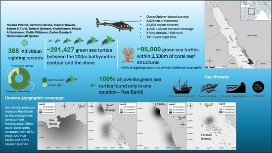
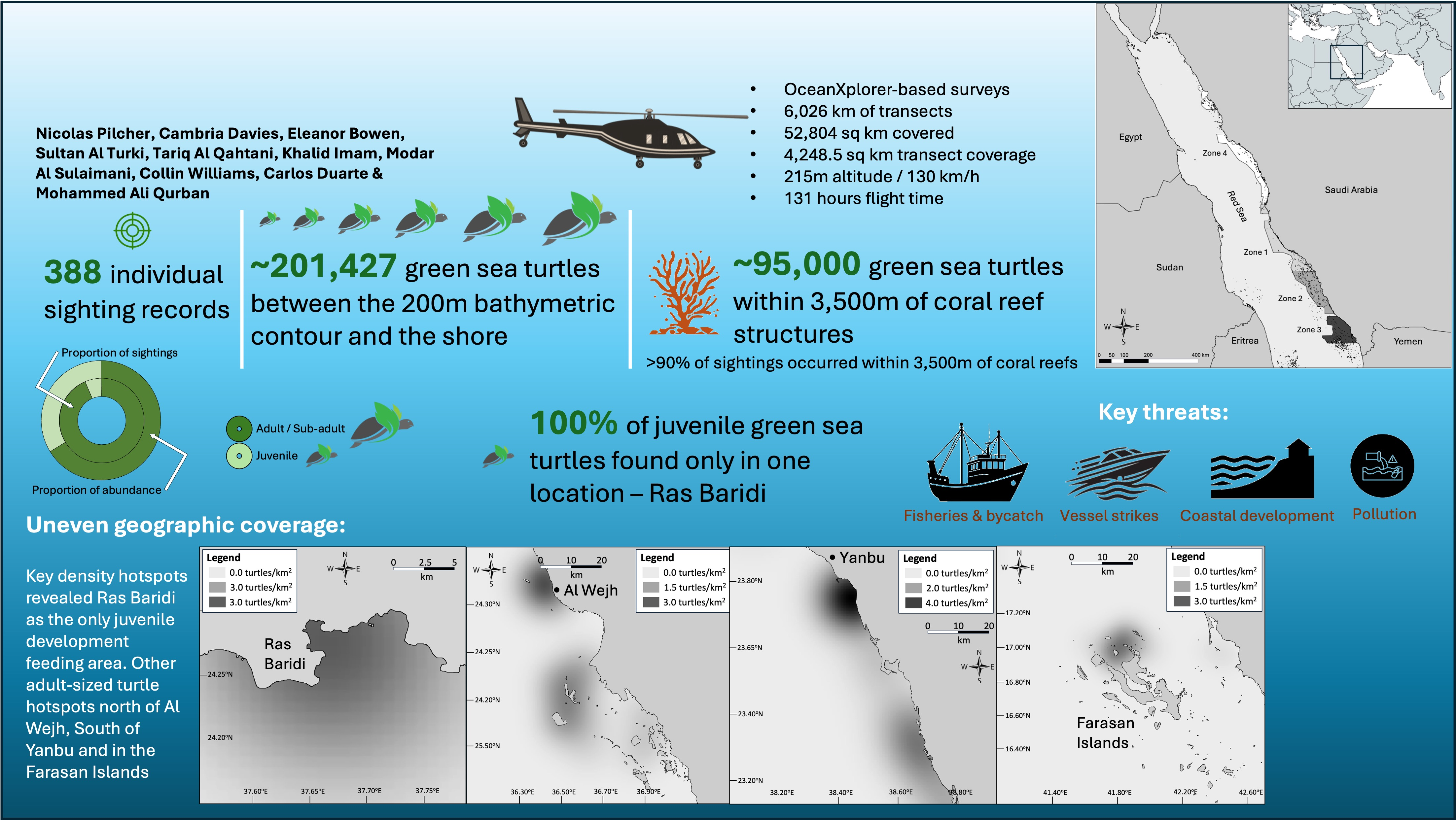
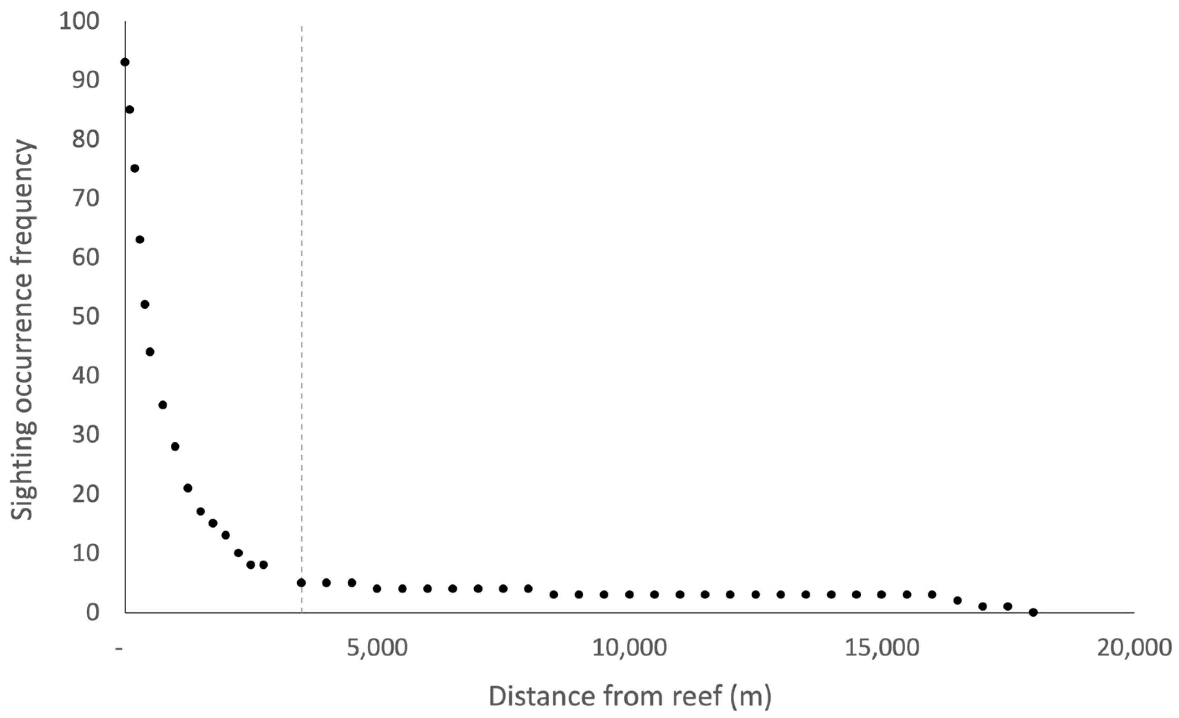
Effective management and conservation of sea turtles is often constrained by a lack of knowledge of at-sea distribution and abundance. While abundance estimates of nesting females are typically well-documented on nesting beaches, counting sea turtles at sea presents challenges due to their widespread distribution and cryptic habits. Given nesting beaches only document adult females, at-sea data are also more informative of greater population demographics. To estimate the abundance and density of green sea turtles (Chelonia mydas) in the Red Sea waters of Saudi Arabia we conducted strip transect aerial surveys in four survey zones that spanned ~66% of shallow water habitats (<200 m depth), within which we counted sea turtles, and also other species such as dugongs and other marine mammals, sharks, and rays. Corresponding abundance estimates were modelled to account for perception bias (whether a surveyor saw a turtle that was available) and detection bias (whether a turtle was available to be seen). Our results suggest an abundance of ~201,427 green sea turtles potentially present between the 200 m bathymetric contour and the Saudi Arabian shore. However, there was a statistically significant relationship between turtle location and proximity to coral reefs, with over 90% of turtles found within 3500 m of coral reef structures (whether coastal fringing reefs, barrier reefs or atolls), and therefore it would be inappropriate to use an estimate assuming equal distribution. Adjusting for this buffer area we estimated ~95,000 turtles (95% CI: 64,000–142,000) within the proximity of reef structures. These findings represent the first abundance estimates of green turtles in the Red Sea. Repeated over time, surveys such as these can identify changes in population structure, distribution and abundance, and inform conservation and management agencies.

1. Introduction

Sea turtles are iconic species that have been under substantive anthropogenic pressures for multiple decades, including bycatch in commercial and artisanal fisheries [1,2], alteration or loss of nesting habitats [3], and both commercial and community-based harvests [4,5]. More recently, the proliferation of marine plastics has also led to turtle mortalities in multiple ocean areas [6,7]. Natural impacts such as climate-related extreme storms [8] and increasing temperature [9] are also influencing sea turtle populations to varying degrees across the globe. However, concerted, informed conservation action has led to the recovery of some species in some areas. For example, the Olive ridley turtle was downlisted from Endangered to Vulnerable on the IUCN Red List in 2008 [10], and the green turtle was downlisted from Endangered to Least Concern on the Red List in 2025 [11]. Despite these conservation successes, other species remain imperilled and Regional Management Units (RMUs) [12] of some species face the threat of imminent extinction (e.g., Eastern and Western Pacific leatherback turtles, Northwest Indian Ocean loggerhead turtles, hawksbill turtles globally).

Science-based management [13,14] is an important component of species conservation, and has been used to guide recovery strategies for multiple species, including the humpback whale in Australia [15], the green sea turtle globally [11], and the Atlantic bluefin tuna [16], amongst others. Indeed, there are multiple cases of species recovery successes in marine conservation, built upon the foundations of robust science-based management and conservation [17]. These management responses involve actions derived from robust data collection, scientific analysis, management interventions, monitoring, and evaluation of management efforts. The present surveys were designed to contribute to science-based management of sea turtles in the Red Sea.

Sea turtle research and population monitoring has predominantly occurred during the easily accessible terrestrial component of sea turtle life histories, when female turtles emerge on nesting beaches to deposit their eggs. However, sea turtles spend the majority of their lives at sea, using various habitats at different life stages including shallow habitats as feeding and development areas, deep-water habitats in early life-stage dispersal, and adult-stage reproduction migrations. These diverse habitats are used as migratory routes, nesting sites, foraging grounds, mating areas, inter-nesting habitat, and as development habitat [18,19]. Understanding sea turtle distribution and abundance in their at-sea environment can address persistent data gaps and greatly contribute to the design of management and conservation efforts.

In Saudi Arabia, interest in sea turtles’ population status was awakened in the 1980s through a joint Saudi Arabia–Australia initiative that resulted in the first robust scientific studies of sea turtles in the Arabian Gulf and (to a lesser extent) the Red Sea [20]. Subsequent to this groundbreaking work, descriptions of sea turtle nesting populations and impacts were documented for the Arabian Gulf [21,22] and the Red Sea [23,24], and estimates of nesting population sizes from that time remain the baselines with which more recent advances in science have been compared [25]. In recent years there has been renewed interest in scientific studies on sea turtles in Saudi Arabia with the establishment of King Abdullah University for Science and Technology (KAUST) in 2009, the development of the Red Sea Project and NEOM giga-projects in 2019, alongside a new environment policy structure and the establishment of the National Center for Wildlife in 2019. Recent work has expanded to studies on turtle habitat use and movements through satellite tracking [26,27,28,29], identification and descriptions of foraging areas [30,31] and new nesting sites [32], implications of climate change [33], genetics [34], threats [35,36] and citizen science [37].

However, with the exception of descriptions of post-nesting adult female migrations [26,27,30], there is minimal information on at-sea abundance and distribution patterns across varying life stages in the Red Sea. Where do juvenile sea turtles recruit and develop in coastal waters? Where do larger sub-adult and adult turtles (both males and females) feed, mate, and disperse? How many turtles are in the Saudi Arabian Red Sea, and how has sea turtle abundance changed over time? To address these questions, the current study provided the first large-scale estimate of abundance and distribution of green sea turtles derived from an aerial survey conducted in 2022 in shallow (<200 m deep) waters in the Saudi Arabian Red Sea. By describing spatial patterns of abundance for turtles inhabiting coastal areas and quantifying a population estimate (i.e., the number of individuals in the study region), we aim to guide the delineation of Important Sea Turtle Areas (IMTAs) [38], national conservation action, and ultimately, long-term monitoring programmes.

2. Materials and Methods

2.1. Flight Logistics

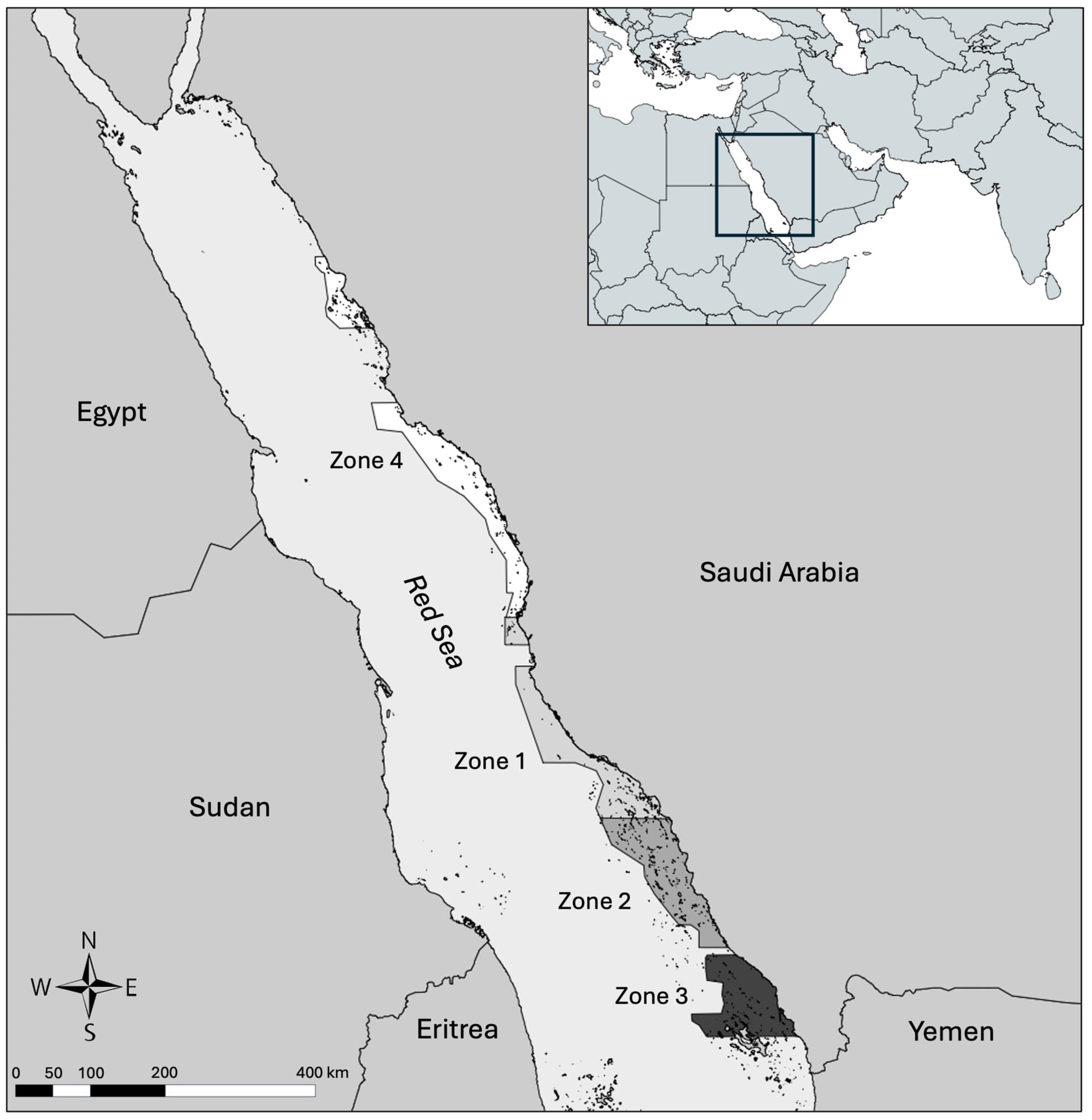
Aerial surveys were conducted between February and May 2022 using an Airbus 125 helicopter (Airbus, Toulouse, France) operated by a single pilot, with one survey leader (front left seat) and two observers (rear left and right seats), with personnel limited due to space and fuel endurance. Flights were only conducted once at each location and along each transect, scheduled within two-week vessel deployments, and subject to weather limitations (no flights were conducted in Beaufort sea state >3). Flight timing and spatial coverage details are provided in Table S1. The helicopter operated off the research vessel OceanXplorer as part of a holistic exploration of the Saudi Arabian Red Sea (the Red Sea Decade Expedition, RSDE). Flights were designed to follow a series of predetermined U-shaped flight plans that spanned a total length of 6804 nm (12,195 km) along the eastern (Saudi Arabian) extent of the Red Sea (Figure 1). The flight plan was superimposed over flight paths from a survey undertaken in the 1980s by Preen [39] for dugongs, so that estimates of current dugong abundance could be tied back to past abundance estimates. However, given the intent of this survey to record multiple species, the flight tracks were extended further offshore from the Preen [39] surveys (Figure S1). Flights were generally oriented in an E-W direction to minimise glare, and environmental data were collected to determine influences on turtle detection. Individual legs were separated by approximately 2 nm (~3.7 km) to avoid double counting animals that might swim and be spotted on adjacent lines. Setting the transects 2 nm apart was designed to minimise this possibility, and also allowed for continuous, manageable track lines to account for the helicopter’s fuel reserves. A reference marker pole extending from either side of the helicopter allowed for a standardised strip transect along the flight path. The effective survey transect width was established via triangulation from the outer extent of the marker pole diagonally to the sea surface, and extended approximately 200 m to either side of the helicopter (400 m total strip width). Strip transects were used instead of distance sampling given limited observer experience, and assumed a constant but declining likelihood of detection across the defined 400 m strip [40,41]. The likelihood of detection was deemed lower on the outer third of the transect strip than in the inner third, where turtles were clearly visible to observers. The rear doors of the helicopter were removed for increased visibility, and each observer recorded their individual sightings into a time-stamped voice recorder, synchronised to the helicopter’s flight recording software. For each green turtle observation, observers recorded whether the survey was ‘on effort’ or ‘off effort’, the time (linked to the helicopter’s GPS track to determine location), the number of individuals, and a size estimate. Size estimates were subjective and classified simply as small or large to refer to juveniles and adults/sub-adults. Given the inability to distinguish between a large sub-adult and an adult, these are referred to hereafter collectively. Sighting data were transcribed independently to written records immediately after each day’s flights. In our surveys, ‘on effort’ refers to the time the helicopter was actively collecting primary data along the designated survey transects. ‘Off effort’ refers to transit, repositioning, or periods where standardised data collection was halted to circle back and identify species, but where sighting data were recorded opportunistically.

Flights were operated at an altitude of 700 ft (~215 m) and a speed of 70 kn (~130 km/h), with course and altitude held by autopilot (Genesys Aerosystems HeliSAS [Moog Inc., Houston, TX, USA], controlled by Garmin GTN650, GTN750 and G500H TXi navigation radios [Garmin Ltd., Olathe, KS, USA]). The autopilot was only disconnected in instances where observer effort was discontinued to circle back for species identification. Given the use of the autopilot, the planned tracks and actual tracks were extremely closely aligned. Flights were typically of ~3 h endurance due to fuel limitations. Records of environmental variables were determined at the start of each flight, and updated based on course changes or changes in environmental conditions as these occurred, using standard categories [42], with the time of each change recorded to the nearest minute. Records were kept of sun altitude (low, medium and high), sun position relative to the helicopter (recorded as hours on a clock face relative to the front of the helicopter), wind and sea state (Beaufort scale), haze (recorded as low, moderate or substantial) and cloud cover in 10% increments. Flight logs from the helicopter provided three-dimensional data on movements and altitude.

Survey areas were split into four zones based on OceanXplorer deployments, and covered a total of 52,804 sq km of the Red Sea, mostly between the shore and the 200 m bathymetric contour line (Figure 1). Due to unforeseen circumstances the surveys planned for the northern Red Sea were discontinued, and due to security concerns, some of the far southern surveys were removed, resulting in a total flight distance of 6026 km and 4248.5 sq km transect coverage over 131 h of flight time.

2.2. Availability Bias (Detection Probability)

Availability bias (i.e., detection probability) pertains to the likelihood of turtles being present in the survey area but being submerged and not available for detection [40,43]. This occurs due to environmental conditions (e.g., sea state, cloud cover, surface glare) and animal characteristics (e.g., body colour and size, diving patterns). Turtles were classified as juvenile or adult/sub-adult subjectively by observers, and referred to as small or large with no ability to measure them from the air. However, smaller turtles were only seen in shallow water habitats where they were easily detected against the sea floor. It is likely that smaller turtles had substantially lower detection probabilities in deeper waters, which may influence the results. Availability (for detection) was determined as the proportion of time green sea turtles spent at different depths at which they could be seen. Proportional time-at-depth data for green turtles in the Red Sea were sourced from ten post-nesting green turtles equipped with satellite transmitters containing time–depth recorders (TDRs), deployed in the northern Red Sea by the NEOM Marine Nature Reserve Department in 2024.

Only data from foraging or inter-nesting behaviour states were used to infer time-at-depth, as turtles frequently surface and breathe during migrations, which could bias detection probability. Data were filtered for time spent within the upper 10 m of the water column, and then by the proportion of time where maximum dive depth was at detection depths of 5 m, 2.5 m and 0.75 m. These depths were chosen as being indicative of decreasing detection probabilities in the inner, middle and outer reaches of the survey transects. We used an inner-weighted distribution for sightings (50:30:20), whereby turtles in the inner third of the transect were more likely to have been seen down to deeper depths than those on outer extents of the strip transect. The Red Sea is generally clear given the lack of terrestrial runoff [44], and thus the detection/depth data were considered indicative of the sighting probabilities for turtles across the entire survey.

Overall, turtles spent 64.7% of their time within the upper 10 m of the water column, within which they spent 27.8% of time in the upper 5 m (inner detection zone), 8.5% of the time in the upper 2.5 m (middle detection zone), and 1.5% of the time in the upper 0.75 m (outer detection zone). While extracted from a small sample of ten turtles, these proportional time-at-depth data are comparable to the detection probabilities from five different studies summarised by Fuentes et al. [43].

Individual-level variation provided bounds for sensitivity analyses. For the inner detection zone, individual means ranged from 20.8% to 56.5%. For the middle and outer detection zones, some individual turtles had no recorded time at these shallow depths during their deployment periods, likely reflecting sampling limitations. We acknowledge that additional Red Sea-specific data on availability bias would strengthen abundance estimates, and urge that these be collected in future surveys.

2.3. Perception Bias

Perception bias results from observers missing turtles that were visible in the survey area, but were not detected and recorded [40,43]. This bias can result from slight inherent variations in observer scanning frequency, observer distraction, or reduced focus on the transect area. Given this survey only employed one set of observers, and it was the first time such surveys had occurred in the Red Sea, we were not able to calculate a perception bias amongst the observers for this study. To solve this, we adapted perception bias from data presented by Fuentes et al. [43] who summarised the findings of multiple other studies in several locations. The probability of an observer detecting an available turtle ranged from 0.37 to 0.93 across studies, with a central estimate of 0.65. We used these values in our sensitivity analyses, applying a correction factor of 1/p for each scenario (where p is the probability of detection), giving correction factors of 2.70 (conservative, p = 0.37), 1.54 (central, p = 0.65), and 1.08 (optimistic, p = 0.93).

We then used a constant probability of detection p = 0.65, or a correction factor of 1/0.65 = 1.538, for each individual sighting record. Fuentes et al. [43] found that perception corrections (single vs. tandem observers) often shifted abundance estimates by only ~5% once availability was applied, and that such small changes often fell within sampling noise. We suggest that perception variability in this study is similarly likely to be within sampling noise ranges once availability is accounted for. We acknowledge that survey-specific data on perception bias would be favourable, and urge that a measure of these be included in future surveys.

2.4. Environmental Conditions Analysis

For each transect we summarised the most frequently recorded (modal) environmental condition and standardised labels for consistency across transects. Sea state was recorded on the Beaufort scale (0 = calm through 4 = moderate breeze and above). Sun altitude was classified in degrees above the horizon as low (0–30°), medium (30–60°), or high (60–90°). Cloud cover was described in 10% increments and categorised as clear (0%), partly cloudy (10–49%), mostly cloudy (50–79%), or overcast (≥80%). Haze was recorded as none, light, moderate, or heavy. The environmental variable classification to determine their effects on abundance estimates are provided in Table S2.

Glare potential was classified by combining sun position relative to the observer with sun altitude: high glare was assigned only when the sun was on the observer’s side of the aircraft and the sun altitude was low or medium; high sun (>60°) was treated as no glare given that glare is minimal when the sun is overhead. Glare was assigned at the sighting level, then summarised to each transect and side (port/starboard).

To test whether glare reduced detection, we compared sightings on the high-glare side of the aircraft versus the opposite side within the same transect using a paired-comparison generalised linear model (GLM). Because both sides of the aircraft shared the same habitat within a transect, any consistent left–right difference under high glare reflected a detection effect rather than habitat variation. We used a log-linear Poisson count model with a log(area/2) offset and transect random effect; over-dispersion was tested to determine whether a Negative Binomial model was required. The result is reported as a rate ratio (high-glare vs. no-glare) with 95% confidence interval.

To assess whether sea state, cloud cover, and haze affected turtle encounter rates across transects, we modelled individuals per transect using a quasi-Poisson GLM with a log(area) offset, including sea state, cloud cover, haze, and zone as fixed effects, plus a day effect. Quasi-Poisson regression was used instead of standard Poisson to account for over-dispersion (variance exceeding the mean) commonly observed in ecological count data, producing more conservative standard errors and confidence intervals. We avoided over-complex model structures (e.g., many interactions) because the data had limited contrast (most flights were calm and clear) and sample sizes were modest. These analyses do not separate perception bias from availability bias; they simply test whether transects flown under different conditions yielded systematically different encounter rates. No perception or availability corrections were applied at this stage; these were handled separately in the abundance estimation.

2.5. Data Analysis

Analyses were conducted using RStudio (version 2024.04.2+764). Estimates of marine turtle relative abundance followed methodology outlined by Pollock et al. [45] that corrects for (1) sampling fraction, (2) perception bias, and (3) availability bias (sensu [40]). Corrections for these biases were applied separately for each turtle sighted as an individual, and for each group of turtles. For each transect we then computed the number of turtles (Σ group_size across all on-effort sightings in the transect); the surveyed area (km²) = area_sq_km per transect (computed from flight path × strip width); the observed density (inds·km⁻²) = turtles sighted/area_sq_km of transect; and summarised means of density (±SE) across survey zones.

To assess the impact of environmental variables on counts and densities, we analysed individual counts and proportions within transects by each environmental factor; and zone mean densities ±SE using the following environmental covariates: sea state, sun altitude, cloud cover, glare, haze, and depth. We then computed Spearman rank correlations (ρ) between transect density (inds·km²) and each ordered environmental factor—sea state, sun altitude, cloud cover, haze (plus depth as numeric)—and repeated the analysis within glare strata (low vs. high) to determine whether any association was simply a by-product of glare. We then fit a linear mixed model with αdayj∼N(0,σday2)\alpha_{\text{day}_j} \sim \mathcal{N}(0, \sigma^2_{\text{day}})αdayj∼N(0,σday2) as a random intercept for zone to handle repeated transects within the same zone; sea, sun, glare are fixed effects (treatment-coded). The Spearman rank correlations provide a robust, assumption-light read on monotonic associations with ordered covariates, while the linear mixed model (LMM) provides a variance-stabilised, zone-adjusted cross-check. We report the Type-II Wald χ² tests (marginal tests for each factor adjusting for the others) and effect estimates with 95% confidence intervals.

2.6. Sensitivity Analysis

To propagate uncertainty through the abundance estimation process and generate confidence intervals, we employed Monte Carlo simulation with 10,000 iterations following the approach of Fuentes et al. [43]. This approach treats five individual turtles as a sample from the population and uses bootstrap resampling to capture uncertainty in availability estimates. For each Monte Carlo iteration, we: (1) assigned each turtle sighting to a detection zone using the 50:30:20 inner-weighted probability distribution, (2) sampled five turtles with replacement from our pool of five individuals to generate a bootstrap estimate of availability for each zone, calculated as the mean of the resampled individual values, (3) sampled a perception probability from a uniform distribution spanning the literature-derived range (0.37–0.93), and (4) calculated a correction factor for each sighting as 1/(availability × perception). Corrected counts were summed and extrapolated to the full survey area using the ratio method. The median and 95% confidence intervals (2.5th and 97.5th percentiles) were extracted from the resulting distribution of 10,000 abundance estimates.

In addition to the bootstrapped confidence intervals, we conducted sensitivity analyses using fixed parameter values to evaluate the influence of key assumptions on abundance estimates and to provide interpretable bounds on plausible estimates. For zone weighting, we compared the inner-weighted distribution (50:30:20) with a uniform distribution (33:33:33). For perception bias, we evaluated three fixed scenarios: conservative (p = 0.37), central (p = 0.65), and optimistic (p = 0.93). For availability bias, we evaluated three fixed scenarios based on individual turtle variation: lower-bound (using minimum non-zero individual means: 20.8%/13.6%/1.5% for inner/middle/outer zones), central (using pooled means: 27.8%/8.5%/1.5%), and upper-bound (using maximum individual means: 56.5%/27.8%/3.5%). The fixed-scenario sensitivity analysis complements the bootstrapped approach by showing how extreme assumptions affect estimates, while the bootstrap provides the primary uncertainty quantification for the central estimate.

2.7. Spatial Analysis and Extrapolation

We determined the distance from each turtle sighting to the nearest reef structure using the Shortest line between features function under Vector geometry in QGIS (https://qgis.org), setting the number of nearest features to 1. The coral reef GIS layer was generated by the Saudi Arabia National Center for Wildlife as a composite of graphically digitised reef outlines from remotely sensed imagery and the Allen Coral Atlas layer (https://allencoralatlas.org).

Abundance estimates were extrapolated from surveyed transects to the full survey area using the ratio method [46]. Given the strong association between turtle sightings and reef structures (>90% within 3500 m of reefs), we calculated extrapolations for: the flight survey zone (52,804 km²), the full 200 m bathymetric zone (79,515 km²), and reef-associated habitat within 3500 m of reef structures (37,422 km²).

3. Results

3.1. Distribution and Abundance of Turtle Sightings—Raw Counts

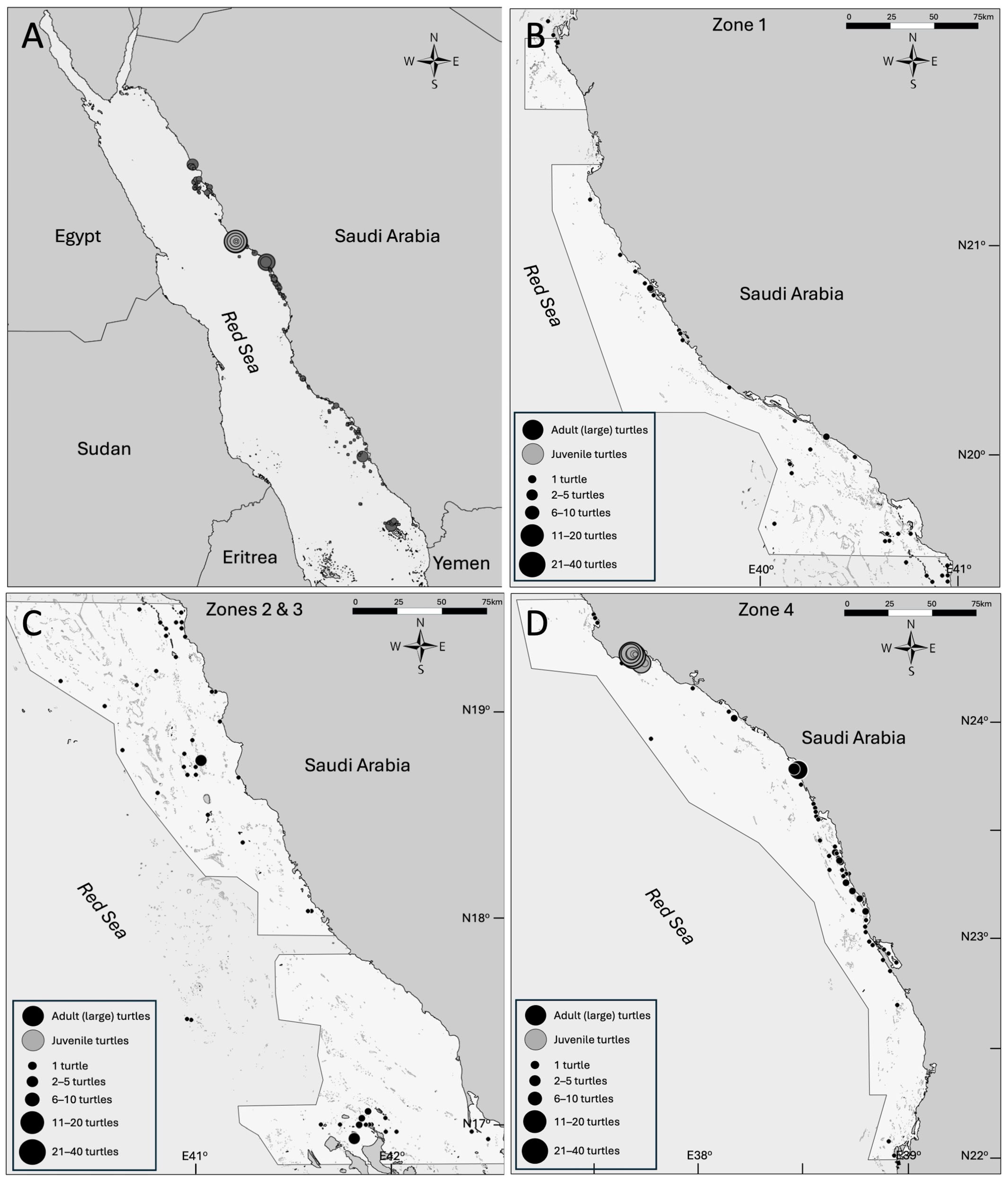
All sea turtle sightings were recorded, including those that did not fall within the transect strip. In such cases, the animals were recorded as effort = “on” or “off” the transect strip to reduce the likelihood of an observer recording a sighting as in the transect when it was just outside. Very few sightings were recorded outside of the survey zones (‘off effort’) and these were not included in density and abundance calculations. A total of 186 sightings comprising 388 individual green turtles were recorded ‘on effort’ during the aerial surveys. The majority of sightings were of single large-sized and presumably large sub-adult or adult turtles, with five larger counts (ranging from 10 to 36 individuals) that comprised nearly entirely juvenile turtles. The distribution and relative abundance of the turtle sightings are presented in Figure 2.

Sightings were distributed relatively evenly along the Red Sea coast, with the exception of a dense accumulation of juvenile turtles southeast of Ras Baridi (grey circles, Figure 2A and Figure S2). This site is the location of the largest mainland nesting site for green sea turtles in the Red Sea [20,24,25]. There were also some elevated densities of large-sized turtles around the northern sector of the Red Sea, south of Yanbu, and in the Farasan Islands.

Of note, the majority of sightings of both adults/sub-adults and juveniles occurred near coral reef formations, with the frequency of sightings declining exponentially with distance from the nearest reef, so that >90% of sightings occurred within 3500 m of coral reef formations, rather than in deeper waters offshore or between reefs (Figure 3). All juveniles were found within the 3500 m coral reef buffers at only one location (southeast of Ras Baridi), but this area also coincided with extensive seagrass habitats. While a number of adult/sub-adult turtle sightings were in shallow waters which may have contained seagrass habitats, many were in deeper waters adjacent to reefs where depths drop vertically to 25–30 m and deeper, where it is unlikely seagrass was present.

3.2. Effects of Environmental Conditions on Detection

3.2.1. Glare

A paired-comparison GLM comparing detection rates between the high-glare and no-glare sides of the aircraft yielded a detection rate ratio of 1.48 (95% CI: 0.85–2.57, p = 0.168). This indicates that turtles on the high-glare side were detected at 1.48 times the rate of the no-glare side; however, this difference was not statistically significant (z = 1.38, p = 0.168; RR = 1.48, 95% CI 0.85–2.57; residual deviance 22.1 on 14 df; AIC 221), and the 95% confidence interval includes 1.0. The model fit was excellent (residual deviance = 22.1 on 14 df; AIC = 221). Only five transects contained high-glare versus no-glare contrasts, providing limited statistical power for this comparison.

The absence of a significant glare effect likely reflects effective mitigation through survey orientation and timing protocols that avoided low sun angles, as well as the restricted range of glare conditions encountered during the survey. Overall, it is believed that glare did not substantially impact the detection of turtles during the surveys.

3.2.2. Sea State, Cloud Cover, and Haze

A quasi-Poisson GLM assessing the effects of sea state, cloud cover, and haze on turtle detection rates across transects found no statistically significant associations between any environmental variable and observed turtle counts (sea state: F_(2,5) = 0.12, p = 0.89; cloud cover: F_(1,5) = 0.05, p = 0.83; haze: F_(2,5) = 2.88, p = 0.15;

Table 1. Rate ratios from quasi-Poisson GLM of environmental effects on turtle detection rates across transects. No terms were statistically significant.

Condition	Rate Ratio	95% CI
Sea State
Very light vs. calm	0.55	0.03–8.75
Light vs. calm	0.003	<0.001–163
Gentle vs. calm	0.004	<0.001–1610
Cloud Cover
Partly cloudy vs. clear	0.07	<0.001–2183
Mostly cloudy vs. clear	3.01	0.003–2761
Overcast vs. clear	1.33	<0.001–6701
Haze
Light vs. none	0.13	<0.001–6056

). All environmental terms produced extremely wide confidence intervals, indicating insufficient statistical power to detect effects. This limitation stems from the restricted range of environmental variability encountered during the survey: 87% of transects were conducted under clear skies, 97% in calm-to-light seas, and adverse conditions were deliberately avoided under survey protocols.

3.2.3. Assessment of Environmental Corrections

None of the environmental variables tested showed a statistically reliable association with observed turtle encounter rates. In line with established practice for strip transect aerial surveys of marine fauna [41,47], environmental conditions were treated as diagnostic covariates rather than correction factors. An environmental correction is applied only when effects are credibly large and consistent across sensitivity checks; this threshold was not met in the present study. Accordingly, no routine environmental adjustment was applied to the abundance estimates. The predominantly favourable survey conditions (calm seas, clear skies, and controlled sun angles) contributed to high-quality data by minimising environmental variation, even though this restricted the range of conditions available for statistical comparison.

3.3. Abundance Estimates

Monte Carlo simulation (n = 10,000 iterations) produced abundance estimates for three spatial extents (

Table 2. Green turtle abundance estimates from Monte Carlo simulation (n = 10,000 iterations) for three spatial extents.

Spatial Extent	Area (km2)	Mean ± SE	95% CI	CV
Flight zone	52,804	133,763 ± 27,683	90,710–199,906	20.7%
Full 200 m zone	79,515	201,427 ± 41,686	136,595–301,028	20.7%
Reef-associated *	37,422	94,797 ± 19,619	64,286–141,672	20.7%

* Primary estimate based on reef-associated habitat.

). Extrapolating to the sum of the four flight survey zones (52,804 km²) yielded an estimate of 133,763 ± 27,683 turtles (95% CI: 90,710–199,906). Extrapolating to the entire 200 m bathymetric zone where turtles could conceivable be distributed (79,515 km²) yielded 201,427 ± 41,686 turtles (95% CI: 136,595–301,028). However, for reef-associated habitat across all of the Saudi Red Sea (37,422 km²), which represents the primary estimate given the strong association between turtle sightings and reef structures, we estimated a mean abundance of 94,797 ± 19,619 (SE) green turtles (95% CI: 64,286–141,672; CV = 20.7%). The corresponding density was 2.53 ± 0.52 turtles per km² within the 3500 m reef buffers.

3.4. Sensitivity Analysis

Sensitivity analyses revealed that availability bias assumptions had the largest effect on abundance estimates (

Table 3. Sensitivity of reef-associated abundance estimates to availability and perception bias assumptions (50:30:20 zone weighting throughout; p = proportion of turtles available for detection).

Availability	p = 0.37	p = 0.65	p = 0.93
Upper-bound	139,214	79,245	55,386
Central	144,754	82,398 *	57,590
Lower-bound	59,567	33,907	23,699

* Primary estimate using central availability and perception values.

). Using lower-bound availability values (higher time at surface) reduced the reef-associated abundance estimate to 33,907 turtles, while upper-bound values yielded 79,245 turtles. Perception bias had a moderate effect, with estimates ranging from 57,590 (p = 0.93) to 144,754 (p = 0.37) turtles. Zone weighting had a smaller effect: uniform weighting (33:33:33) increased the estimate to 121,552 turtles compared to 82,398 with inner-weighted (50:30:20) distribution.

The full range of estimates across all sensitivity scenarios (23,699 to 144,754 turtles) reflects a 6.1-fold difference, with availability bias contributing approximately 2.4-fold variation and perception bias contributing approximately 2.5-fold variation. The Monte Carlo 95% confidence interval (64,286–141,672) captures much of this uncertainty while accounting for the correlation structure among parameters.

4. Discussion

The current study provides the first bias-corrected abundance estimate for green turtles in the Saudi Arabian Red Sea, suggesting approximately 95,000 individuals (95% CI: 64,000–142,000) occur within reef-associated habitat, and some 200,000 (95% CI: 136,595–301,028) may occur from the shore to the 200 m bathymetric zone. Our estimates account for both perception bias (observers missing available turtles) and availability bias (turtles being submerged and unavailable for detection), following the methodological framework established by Marsch & Sinclair [40,41] and expanded on by Fuentes et al. [43].

The large-scale aerial survey helped identify and confirm purported hotspots of juvenile and adult/sub-adult green turtle abundance in the eastern Red Sea, where they face many ongoing threats, including harvest, entanglement, vessel strikes, pollution, and other anthropogenic stressors [48,49,50,51]. There are also risks of noise [52], vessel strikes and oil pollution from the intense shipping that passes thorough this vital geopolitical waterway [53]. Recent surveys in 2024 and 2025 by the King Abdullah University for Science and Technology (KAUST) on behalf of the National Center for Wildlife (NCW) have demonstrated that commercial fishery bycatch extending south of Al Lith towards the Farasan Islands is a worrying and ongoing threat to sea turtles in the Red Sea (NCW, unpublished report). There are also some 3800 small artisanal vessels distributed across 34 fishing ports along the entire Red Sea coast that may additionally impact sea turtles. NCW stranding data also indicate 81 turtles were reported stranded in the Red Sea between 2019 and 2023 (NCW, unpublished data) and it is likely the majority of these were the result of bycatch in commercial and artisanal fisheries. With the exception of turtles in the Farasan Islands Marine Protected Area, no other major aggregations were recorded inside protected areas during these surveys. Importantly, the shallow bay southeast of Ras Baridi, where all juvenile turtles were found, is not protected and yet is likely a key source of sub-adult and adult turtles in the Saudi Arabian Red Sea. The NCW has a broad mandate to conserve terrestrial and marine wildlife in Saudi Arabia, and the General Organisation for the Conservation of Coral Reefs and Turtles in the Red Sea (SHAMS) has a specific mandate to protect sea turtles identified in this study. Additionally, the Directorate of Fisheries under the Ministry of Environment, Water and Agriculture (MEWA) is responsible for fisheries management, which is known to directly impact sea turtles in the Red Sea. Addressing bycatch and protection of feeding and nesting habitats by these agencies remain the highest-priority measures for the conservation of sea turtles in the Saudi Arabian Red Sea.

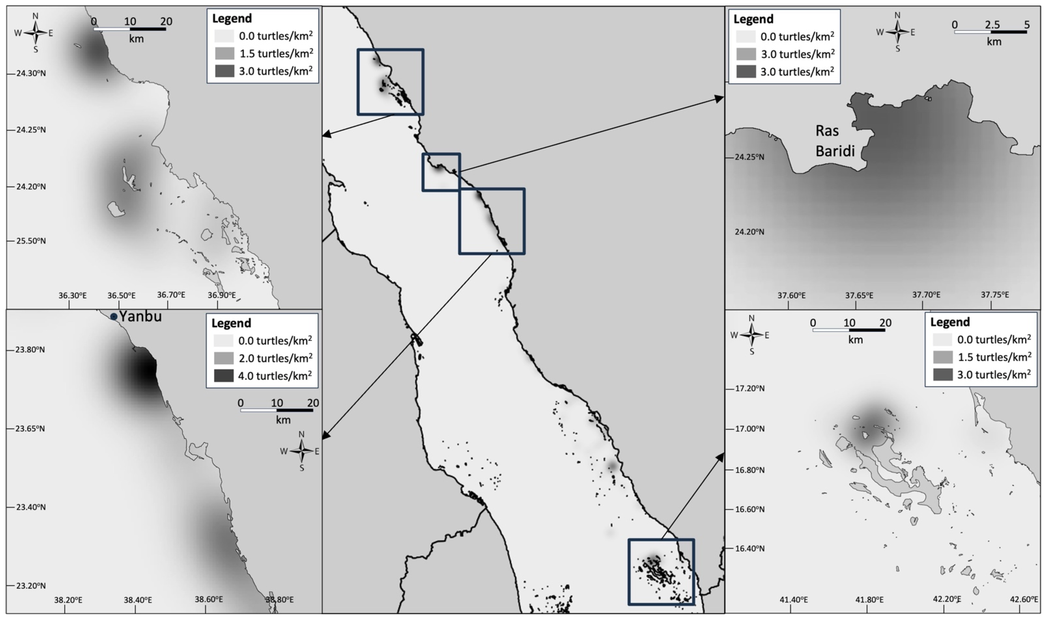
Given the risk of vessel strikes for turtles on the surface [54,55], mapping the density of turtles in shallow coastal waters can also aid in the design of go-slow zones and vessel exclusion areas, and highlight areas where at-sea protection of sea turtles is most warranted. While at a Red Sea basin-wide level the distribution was wide and overall density estimates were low, several hotspot areas were identified (Figure 4). These areas also merit consideration for conservation and management attention by Saudi authorities, in particular the zone to the SE of Ras Baridi which appears to be an important juvenile development area for green turtles in the Saudi Arabian Red Sea.

The overall density estimates for turtles averaged 2.51 ± 0.52 turtles/km² across the Red Sea basin, with increased densities within the lagoon SE of Ras Baridi, primarily comprising juvenile turtles (Figure 4). We acknowledge that the subjective assessment of turtle size (and thus age class) may have introduced a level of error in the distinction between juvenile and adult/sub-adult turtles, but given the smaller turtles were only spotted on one flight and at one location, and the observers were able to clearly distinguish between the larger turtles (adults and large sub-adults typically measure 80–100 cm in curved carapace lengths) and the smaller juveniles (that generally measure <60 cm) during this flight, we believe this error would have been minimal across all of the survey. Our abundance estimates should also be considered alongside the annual number of nesting green turtles in Saudi Arabia [25], and also at other nesting sites such as in Egypt [56,57], that likely number between 500 and 1000 annual nesters [58]. With an age to maturity that can range from 28 [59] to 40 [60] years and typical clutch frequencies of 3 to 6 [61], clutch sizes of ~100 eggs [23] and a hatching success of 40% [33] to 80% [23], the green turtle population in the Red Sea likely produces a range of 60,000 to 480,000 hatchlings annually. While the study identified primarily larger-sized sub-adult and adult turtles (with the exception of the single dense foraging and development area for smaller juvenile turtles south of Ras Baridi), the abundance estimate of approximately 95,000 individuals appears reasonable after natural and anthropogenic mortality are taken into account. Our findings are also consistent with the order of magnitude of estimates developed by Fuentes et al. [47] for the northern Great Barrier Reef, Australia.

Some nesting turtles from the Saudi Arabian nesting sites in the north of the Saudi Red Sea remain in Saudi waters upon their return migration after the nesting season [26,27,28,29], while others travel to Egypt, Sudan and Eritrea. There is no data on migrations to and from nesting sites in the south of Saudi Arabia, and it is possible this survey detected some nesting turtles that may have been from outside Saudi waters, along with a greater majority of resident turtles. The phenology of nesting in the Red Sea advances along a south-to-north gradient, with nesting in the southern Red Sea commencing as early as February to March, and in the northern Red Sea from about August onward [25]. Given this timing, the aerial surveys overlapped slightly with nesting in the southern Red Sea (indeed, some evidence of nesting was observed on several islands); it is possible some of the larger turtles may have been ‘visiting’ nesting adults and not full-time residents. The aerial surveys were concluded by the time the onset of nesting occurred at the larger northern sites (see [25]), and we believe that the overlap with the nesting season and the potential arrival of nesters from foraging areas outside of the Saudi Red Sea waters at these sites was minimal and would not largely bias the abundance estimates and confound resident and visiting nesters. We acknowledge that surveys during and outside of nesting seasons would resolve abundance estimate discrepancies and, given the phased south-to-north onset of nesting, it is likely that only surveys from November to February would exclude nesting turtles, and any surveys conducted from March to October would include both resident and outside visitors. These considerations should be included in the design of future survey campaigns.

The strong association between turtle sightings and reef structures (>90% within 3500 m) also supports focusing abundance estimates on reef-associated habitat rather than extrapolating uniformly across the entire survey area during future surveys. Given the steep bathymetric gradients in the Red Sea, this spatial pattern is consistent with green turtle foraging ecology, as they rely on seagrass beds and algal communities, typically associated with shallow water habitats [62]. The identification of only one hotspot for juvenile turtles (in the bay south of Ras Baridi) suggests that this is a critically important site for management and conservation of the species, requiring immediate attention.

Availability bias had the largest influence on abundance estimates in our sensitivity analyses, and this finding is consistent with Fuentes et al. [43]. Our use of locally collected TDR data from Red Sea green turtles represents an improvement over extrapolating availability parameters from other geographic regions. We found that the sensitivity analysis results for both perception and availability bias, and for detection zones, were broadly within the range of the confidence interval in Monte Carlo simulations, suggesting the abundance estimates were reliable even in the face of small sample sizes of turtles to calculate availability bias, and the lack of multiple sets of observers to calculate perception bias. Nonetheless, the limited sample size remains a constraint that should be addressed in future studies, potentially through Secchi disc trials [47] in cases where TDR data remain unavailable. The coefficient of variation (20.7%) reflects substantial but manageable uncertainty, primarily driven by individual variation in turtle diving behaviour among our limited sample of TDR-tagged animals. This level of precision is comparable to other marine megafauna aerial surveys and sufficient for baseline population assessment and trend monitoring.

Several additional limitations should be considered when interpreting these results. First, the TDR data came from satellite-relayed devices with coarse depth resolution (10 m bins), requiring assumptions about time allocation within the upper 10 m. Second, we lacked individual sighting position data within transects, necessitating probabilistic zone assignment rather than direct measurement. Third, perception bias was estimated from the literature values rather than survey-specific mark–recapture analysis. Future surveys could address these limitations by deploying higher-resolution TDR devices, recording sighting positions within transects, and implementing tandem observer protocols for perception bias estimation.

Despite these limitations, the current study established an important baseline for green turtle abundance in the Saudi Arabian Red Sea and a replicable survey approach for basin-scale monitoring of regional sea turtle populations. Repeated surveys using consistent methodology will enable trend detection and inform adaptive management of this ecologically significant population. The surveys also provided data on the distribution and abundance of dugongs, whales, multiple dolphin species, whale sharks and manta rays, and as such are an efficient method to collect data on multiple species, which can be used to design effective management and conservation efforts.

References

1. Lewison, R.L.; Crowder, L.B.; Read, A.J.; Freeman, S.A. Understanding impacts of fisheries bycatch on marine megafauna. Trends Ecol. Evol. 2004, 19, 598–604. [Google Scholar] [CrossRef]
2. Senko, J.F.; Nalovic, M.A. Addressing sea turtle bycatch in developing countries: A global challenge that requires adaptive solutions for the 21st Century. In Sea Turtle Research and Conservation; Nahill, B., Ed.; Academic Press: New York, NY, USA, 2021; pp. 151–165. [Google Scholar]
3. Sella, K.A.N.; Fuentes, M.M.P.B. Exposure of marine turtle nesting grounds to coastal modifications: Implications for management. Ocean Coast. Manag. 2019, 169, 182–190. [Google Scholar] [CrossRef]
4. Frazier, J. Marine turtles: The role of flagship species in interactions between people and the sea. Mar. Stud. 2005, 4, 5–38. [Google Scholar]
5. Van Houtan, K.S.; Kittinger, J.N. Historical commercial exploitation and the current status of Hawaiian green turtles. Biol. Conserv. 2014, 170, 20–27. [Google Scholar] [CrossRef]
6. Nelms, S.E.; Duncan, E.M.; Broderick, A.C.; Galloway, T.S.; Godfrey, M.H.; Hamann, M.; Lindeque, P.K.; Godley, B.J. Plastic and marine turtles: A review and call for research. ICES J. Mar. Sci. 2016, 73, 165–181. [Google Scholar]
7. Moon, Y.; Shim, W.J.; Hong, S.H. Characteristics of plastic debris ingested by sea turtles: A comprehensive review. Ocean Sci. J. 2023, 58, 31. [Google Scholar] [CrossRef]
8. Van Houtan, K.S.; Bass, O.L. Stormy oceans are associated with declines in sea turtle hatching. Curr. Biol. 2007, 17, 590–591. [Google Scholar] [CrossRef]
9. Maurer, A.S.; Seminoff, J.A.; Layman, C.A.; Stapleton, S.P.; Godfrey, M.H.; Reiskind, M.O.B. Population viability of sea turtles in the context of global warming. BioScience 2021, 71, 790–804. [Google Scholar] [CrossRef]
10. Abreu-Grobois, A.; Plotkin, P.; IUCN SSC Marine Turtle Specialist Group. Lepidochelys olivacea. In The IUCN Red List of Threatened Species; IUCN: Cambridge, UK, 2008; p. e.T11534A3292503. [Google Scholar] [CrossRef]
11. Wallace, B.P.; Broderick, A.C. Chelonia mydas. In The IUCN Red List of Threatened Species; IUCN: Cambridge, UK, 2025; p. e.T4615A285108125. [Google Scholar] [CrossRef]
12. Wallace, B.P.; Posnik, Z.A.; Hurley, B.J.; DiMatteo, A.D.; Bandimere, A.; Rodriguez, I.; Maxwell, S.M.; Meyer, L.; Brenner, H.; Jensen, M.P.; et al. Marine turtle regional management units 2.0: An updated framework for conservation and research of wide-ranging megafauna species. Endanger. Species Res. 2023, 52, 209–223. [Google Scholar] [CrossRef]
13. Sutherland, W.J.; Pullin, A.S.; Dolman, P.M.; Knight, T.M. The need for evidence-based conservation. Trends Ecol. Evol. 2004, 19, 305–308. [Google Scholar] [CrossRef] [PubMed]
14. Mahajan, S.L.; Tanner, L.; Ahmadia, G.; Becker, H.; DeMello, N.; Fidler, R.; Harborne, A.R.; Jagadish, A.; Mills, M.; Cairney, P.; et al. Accelerating evidence-informed decision-making in conservation implementing agencies through effective monitoring, evaluation, and learning. Biol. Conserv. 2023, 286, 110304. [Google Scholar]
15. Bejder, M.; Johnston, D.W.; Smith, J.; Friedlaender, A.; Bejder, L. Embracing conservation success of recovering humpback whale populations: Evaluating the case for downlisting their conservation status in Australia. Mar. Policy 2016, 66, 137–141. [Google Scholar] [CrossRef]
16. Porch, C.; Bonhommeau, S.; Diaz, G.A.; Arrizabalaga, H.; Melvin, G. The journey from overfishing to sustainability for Atlantic bluefin tuna, Thunnus thynnus. In The Future of Bluefin Tunas; Block, B.A., Ed.; Johns Hopkins University Press: Baltimore, MD, USA, 2017; pp. 3–44. [Google Scholar]
17. Rossbach, S.; Steckbauer, A.; Klein, S.G.; Arossa, S.; Geraldi, N.R.; Lim, K.K.; Martin, C.; Rossbach, F.I.; Shellard, M.J.; Valluzzi, L.; et al. A tide of change: What we can learn from stories of marine conservation success. One Earth 2023, 6, 505–518. [Google Scholar] [CrossRef]
18. Musick, J.A.; Limpus, C.J. Habitat utilization and migration in juvenile sea turtles. In The Biology of Sea Turtles; Musick, J.A., Lutz, P.L., Eds.; CRC Press: Boca Raton, FL, USA, 1997; pp. 137–163. [Google Scholar]
19. Plotkin, P.; Lutz, P.L.; Musick, J.A.; Wyneken, J. Adult migrations and habitat use. In The Biology of Sea Turtles; Musick, J.A., Lutz, P.L., Eds.; CRC Press: Boca Raton, FL, USA, 2003; Volume II, pp. 225–241. [Google Scholar]
20. Miller, J.D. Marine Turtles, Volume 1: An Assessment of the Conservation Status of Marine Turtles in the Kingdom of Saudi Arabia; Report No. 9; MEPA: Jeddah, Saudi Arabia, 1989; p. 289. [Google Scholar]
21. Pilcher, N.J. The hawksbill turtle, Eretmochelys imbricata, in the Arabian Gulf. Chelonian Conserv. Biol. 1999, 3, 312–317. [Google Scholar]
22. Pilcher, N.J. The green turtle, Chelonia mydas, in the Saudi Arabian Gulf. Chelonian Conserv. Biol. 2000, 3, 730–734. [Google Scholar]
23. Al-Merghani, M.; Miller, J.D.; Pilcher, N.J.; Al-Mansi, A. The green and hawksbill turtles in the Kingdom of Saudi Arabia: Synopsis of nesting studies 1986–1997. Fauna Arab. 2000, 18, 369–384. [Google Scholar]
24. Pilcher, N.J.; Al-Merghani, M. Reproductive biology of the green turtle Chelonia mydas at Ras Baridi, Saudi Arabia. Herpetol. Rev. 2000, 32, 142–147. [Google Scholar]
25. Shimada, T.; Meekan, M.G.; Baldwin, R.; Al-Suwailem, A.M.; Clarke, C.; Santillan, A.S.; Duarte, C.M. Distribution and temporal trends in the abundance of nesting sea turtles in the Red Sea. Biol. Conserv. 2021, 261, 109235. [Google Scholar] [CrossRef]
26. Al-Mansi, A.M.; Sambas, A.Z.; Abukaboos, B.A.; Al Zahrani, A.H.; Abdulaziz, A.S.; Almasabi, A.A.; Alkreda, R.S.; Miller, J. Satellite tracking of post-nesting green sea turtles (Chelonia mydas) from Ras Baridi, Red Sea. Front. Mar. Sci. 2021, 8, 758592. [Google Scholar] [CrossRef]
27. Shimada, T.; Duarte, C.M.; Al-Suwailem, A.M.; Tanabe, L.K.; Meekan, M.G. Satellite tracking reveals nesting patterns, site fidelity and potential impacts of warming on major green turtle rookeries in the Red Sea. Front. Mar. Sci. 2021, 8, 633814. [Google Scholar] [CrossRef]
28. Tanabe, L.K.; Cochran, J.E.M.; Berumen, M.L. Inter-nesting, migration, and foraging behaviors of green turtles (Chelonia mydas) in the central-southern Red Sea. Sci. Rep. 2023, 13, 11222. [Google Scholar]
29. Tanabe, L.K.; Cochran, J.E.M.; Williams, C.T.; Garzon, F.; Langner, U.; Hardenstine, R.S.; Hawkes, L.A.; Brainard, R.E.; Eweida, A.A.; Marshall, P.A.; et al. Case report: Tracking data from foraging hawksbill turtles in the northern Red Sea. Anim. Biotelem. 2023, 11, 1. [Google Scholar] [CrossRef]
30. Mann, H.F.; Wildermann, N.E.; Fu, C.; Barrios-Garrido, H.; Shimada, T.; Pluma, N.; Duarte, C.M. Green turtle tracking leads the discovery of seagrass blue carbon resources. Proc. R. Soc. B 2024, 291, 20240502. [Google Scholar] [CrossRef]
31. Garzon, F.; Williams, C.T.; Cochran, J.E.; Tanabe, L.K.; Abdulla, A.; Berumen, M.L.; Hawkes, L.A. A multi-method characterization of Elasmobranch & Cheloniidae communities of the north-eastern Red Sea and Gulf of Aqaba. PLoS ONE 2022, 17, e0275511. [Google Scholar]
32. Scott, K.; Tanabe, L.K.; Miller, J.D.; Berumen, M.L. Newly described nesting sites of the green sea turtle (Chelonia mydas) and the hawksbill sea turtle (Eretmochelys imbricata) in the central Red Sea. PeerJ 2022, 10, e13408. [Google Scholar] [CrossRef] [PubMed]
33. Tanabe, L.; Ellis, J.; Elsadek, I.; Berumen, M. Potential feminization of Red Sea turtle hatchlings as indicated by in situ sand temperature profiles. Conserv. Sci. Pract. 2020, 2, e266. [Google Scholar]
34. Scott, K.; He, S.; Hardenstine, R.S.; Tanabe, L.K.; Barrios-Garrido, H.; Jensen, M.P.; Afiq-Rosli, L.; Wildermann, N.E.; Duarte, C.M.; Cochran, J.E.; et al. Genetic divergence and isolation of the green sea turtle (Chelonia mydas) in the Red Sea. Trends Ecol. Evol. 2025, 15, e72046. [Google Scholar] [CrossRef]
35. Tanabe, L.K.; Carvalho, S.; Dasari, V.; Nasif, A.; O’Toole, K.A.; Berumen, M.L. Potential effects of heavy metal pollution from a cement factory near Saudi Arabia’s largest green turtle rookery. Environ. Monit. Assess. 2022, 194, 450. [Google Scholar] [CrossRef]
36. Tanabe, L.K.; Cochran, J.E.M.; Hardenstine, R.S.; Scott, K.; Berumen, M.L. A preliminary report of plastic ingestion by hawksbill and green turtles in the Saudi Arabian Red Sea. Anim. Sci. 2023, 13, 314. [Google Scholar]
37. Montagna, M.I.; Alatawi, A.B.; Algohane, A.; Alturki, S.; Barrios-Garrido, H.; Mancini, A.; Al Mansi, A.H.; Eamalho, R.O.; Taher, A.R.; Al Zahrani, A.; et al. Combined photo identification and flipper tagging of green turtles identify connections between Egyptian Red Sea feeding areas and a key nesting area in Saudi Arabia. Indian Ocean Turt. Newsl. 2023, 38, 2–7. [Google Scholar]
38. Bandimere, A.; Brenner, H.; Casale, P.; DiMatteo, A.; Hurley, B.; Hutchinson, B.; Mast, R.; Maxwell, S.; Meyer, L.; Poznik, Z.; et al. Important Marine Turtle Areas; IUCN SSC Marine Turtle Specialist Group Guidelines 1.0; IUCN: Cambridge, UK, 2021; 12p. [Google Scholar]
39. Preen, A. The Status and Conservation of Dugongs in the Arabian Region; Report No 10; Meteorology and Environment Protection Administration: Jeddah, Saudi Arabia, 1989; 200p. [Google Scholar]
40. Marsh, H.; Sinclair, D.F. Correcting for visibility bias in strip transect aerial surveys of aquatic fauna. J. Wildl. Manag. 1989, 53, 1017–1024. [Google Scholar] [CrossRef]
41. Marsh, H.; Sinclair, D.F. An experimental evaluation of dugong & sea turtle aerial survey techniques. Aust. Wildl. Res. 1989, 16, 639–650. [Google Scholar]
42. Sobtzick, S.; Hagihara, R.; Penrose, H.; Grech, A.; Cleguer, C.; Marsh, H. An assessment of the distribution and abundance of dugongs in the Northern Great Barrier Reef and Torres Strait. In Report to the National Environmental Research Program; Reef and Rainforest Research Centre Limited: Cairns, Australia, 2014; 72p. [Google Scholar]
43. Fuentes, M.M.P.B.; Bell, I.; Hagihara, R.; Hamann, M.; Hazel, J.; Huth, A.; Seminoff, J.A.; Sobtzick, S.; Marsh, H. Improving in-water estimates of marine turtle abundance by adjusting aerial survey counts for perception and availability biases. J. Exp. Mar. Biol. Ecol. 2015, 471, 77–83. [Google Scholar] [CrossRef]
44. Cai, C.; Huertas, A.D.; Agusti, S. Declining nutrient availability and metal pollution in the Red Sea. Commun. Earth Environ. 2023, 4, 424. [Google Scholar] [CrossRef]
45. Pollock, K.H.; Marsh, H.D.; Lawler, I.R.; Alldredge, M.W. Estimating animal abundance in heterogeneous environments: An application to aerial surveys for dugongs. J. Wildl. Manag. 2006, 70, 255–262. [Google Scholar] [CrossRef]
46. Jolly, G.M. Sampling methods for aerial censuses of wildlife populations. East Afr. Agric. For. J. 1969, 34, 46–49. [Google Scholar] [CrossRef]
47. Marsh, H.; Saalfeld, W.K. Aerial surveys of sea turtles in the northern Great Barrier-Reef Marine Park. Wildl. Res. 1989, 16, 239–249. [Google Scholar] [CrossRef]
48. Kattan, A.; Coker, D.J.; Berumen, M.L. Reef fish communities in the central Red Sea show evidence of asymmetrical fishing pressure. Mar. Biodivers. 2017, 47, 1227–1238. [Google Scholar] [CrossRef]
49. Shellem, C.T.; Ellis, J.I.; Coker, D.J.; Berumen, M.L. Red Sea fish market assessments indicate high species diversity and potential overexploitation. Fish. Res. 2021, 239, 105922. [Google Scholar] [CrossRef]
50. Womersley, F.C.; Rohner, C.A.; Abrantes, K.; Afonso, P.; Arunrugstichai, S.; Bach, S.S.; Bar, S.; Barash, A.; Barnes, P.; Barnett, A.; et al. Identifying priority sites for whale shark ship collision management globally. Sci. Total Environ. 2024, 934, 172776. [Google Scholar] [CrossRef]
51. Williams, C.; Foster, A.D.; Kattan, A.; Cochran, J.E.; Berumen, M.L. Float lines from the Arabian trap fishery are an overlooked entanglement risk for marine turtles. Reptil. Amphib. 2025, 32, e23092. [Google Scholar] [CrossRef]
52. Larayedh, R.; Cornuelle, B.D.; Krokos, G.; Hoteit, I. Numerical investigation of shipping noise in the Red Sea. Sci. Rep. 2024, 14, 5851. [Google Scholar] [CrossRef]
53. Mittal, H.V.R.; Langodan, S.; Zhan, P.; Li, S.; Knio, O.; Hoteit, I. Hazard assessment of oil spills along the main shipping lane in the Red Sea. Sci. Rep. 2021, 11, 17078. [Google Scholar] [CrossRef] [PubMed]
54. Fuentes, M.M.; Meletis, Z.A.; Wildermann, N.E.; Ware, M. Conservation interventions to reduce vessel strikes on sea turtles: A case study in Florida. Mar. Pol. 2021, 128, 104471. [Google Scholar]
55. Welsh, R.C.; Witherington, B.E. Spatial mapping of vulnerability hotspots: Information for mitigating vessel-strike risks to sea turtles. Glob. Ecol. Conserv. 2023, 46, e02592. [Google Scholar] [CrossRef]
56. Hanafy, M. Nesting of marine turtles on the Egyptian beaches of the Red Sea. Egypt. J. Aquat. Biol. Fish. 2012, 16, 59–71. [Google Scholar] [CrossRef]
57. Mohammad, A.S.; Hussein, H.N.; Ghallab, A.; Mahdy, A.; Madkour, H. Status of green sea turtles (Chelonia mydas) at Zabargad Island, southern Egyptian Red Sea. In Coral Reefs and Associated Marine Fauna Around the Arabian Peninsula; CRC Press: Boca Raton, FL, USA, 2024; pp. 323–329. [Google Scholar]
58. Tanabe, L.; Hardenstine, R.; Cornfield, C.; Shum, E.; Rees, A.L.; Baldwin, R. KSA Outlook Turtle Report 2024; 5Oceans: Muscat, Oman, 2024; 233p. [Google Scholar]
59. Van Houtan, K.S.; Hargrove, S.K.; Balazs, G.H. Modeling sea turtle maturity age from partial life history records. Pac. Sci. 2014, 68, 465–477. [Google Scholar] [CrossRef]
60. Goshe, L.R.; Avens, L.; Scharf, F.S.; Southwood, A.L. Estimation of age at maturation and growth of Atlantic green turtles (Chelonia mydas) using skeletochronology. Mar. Biol. 2010, 157, 1725–1740. [Google Scholar] [CrossRef]
61. Weber, N.; Weber, S.B.; Godley, B.J.; Ellick, J.; Witt, M.; Broderick, A.C. Telemetry as a tool for improving estimates of marine turtle abundance. Biol. Conserv. 2013, 167, 90–96. [Google Scholar] [CrossRef]
62. Bjorndal, K.A. Foraging ecology and nutrition of sea turtles. In The Biology of Sea Turtles; CRC Press: Boca Raton, FL, USA, 2017; Volume I, pp. 199–231. [Google Scholar]
Figure 1. Map of the Red Sea depicting the four aerial survey zones along the Saudi Arabian coast.
Ecologies 07 00050 g001
Figure 2. Distribution and relative abundance of green sea turtles from raw sightings. (A) Overall distribution in the Saudi Arabian Red Sea; (B) distribution in the central north (Zone 1); (C) distribution in the central south (Zone 2) and south (Zone 3); (D) distribution in the central Red Sea (Zone 4). Grey lines represent coral reef formations. Concentric circles at Ras Baridi indicate multiple sightings of different numbers of turtles.
Ecologies 07 00050 g002
Figure 3. Relationship between sightings and distance to reef formations. Dashed line represents 3500 m from the closest reef.
Ecologies 07 00050 g003
Figure 4. Kernel density distribution map showing hotspot locations where green turtles in the Saudi Arabian Red Sea may be subject to higher risk of vessel strikes (note: scales differ for each hotspot graphic).
Ecologies 07 00050 g004