Assessment of Diversity and Evenness of Herbaceous Vegetation and Natural Regeneration Communities in the Plaiul Fagului Reserve

Abstract

Environmental changes and anthropogenic pressures significantly influence both the tree layer and natural regeneration within forest ecosystems. Protected areas represent essential territories for the maintenance and conservation of species within forest communities. In this context, the present study aims to develop a methodological framework for the integrated application of diversity, evenness, and dominance indices in the study of forest plant communities. Analyses were conducted at both α- and β-diversity levels, providing a methodological basis for characterizing local diversity and community differentiation. Species diversity was estimated using the Shannon–Wiener (H′) and Simpson (D) indices, while evenness and dominance were assessed using the Pielou (J′) and Berger–Parker (d) indices. Differences among communities were quantified using the Bray–Curtis dissimilarity index and its components, turnover and nestedness, and structural convergence of forest communities was analyzed through the ICF. The results indicate that α-diversity, estimated by H′, ranges from low to moderate, suggesting a relatively uniform distribution of species abundance. In certain microhabitats, processes of diversification and oligodominance are observed. At the β-diversity level, the analyzed communities are characterized by high dissimilarity, mainly driven by species turnover and, to a lesser extent, by nestedness associated with species loss. The ICF highlights that these forest communities exhibit relatively high structural uniformity, characteristic of mature stands in ecological equilibrium.

1. Introduction

The herbaceous layer and natural regeneration represent dynamic and sensitive components of forest ecosystems, reflecting the variability of local ecological conditions and influencing forest functioning. Through their roles in nutrient cycling, microclimate regulation, and support of regeneration, herbaceous species contribute to ecosystem stability and provide early indicators of structural changes driven by natural or anthropogenic factors [1,2,3,4,5].

The composition and structure of the herbaceous layer result from the interaction between abiotic factors, available resources, and disturbance intensity, being influenced by light availability, water regime, stand composition, and anthropogenic pressure. These relationships shape diversity patterns and regeneration processes, conferring high ecological value to the herbaceous layer for monitoring forest ecosystem dynamics [6,7,8].

Heterogeneous forest habitats, through microsite variation and differentiated resource distribution, promote higher plant richness by expanding ecological niches and reducing interspecific competition [9,10]. In contrast, anthropogenic activities such as selective logging, overgrazing, or climate change can reduce understorey diversity, affecting regeneration and the functional balance of the forest. Maintaining a plant composition adapted to local conditions is therefore essential for the stability of forest ecosystems [11,12].

The analysis of forest vegetation diversity increasingly relies on quantitative methods that employ ecological indices to integrate information on species abundance and distribution. These indices provide a comprehensive perspective on the organization of plant communities and the relationships between floristic structure, natural regeneration, and ecological processes within ecosystems [13,14]. Among them, dominance indices such as Simpson, McIntosh, and Berger–Parker quantify the distribution of abundance among species, while Pielou, Shannon–Wiener, Gini, and Camargo coefficients assess the evenness of plant communities and the level of ecological dominance [15]. Simultaneously, our Integrated Community Structure Index combines species turnover, community evenness, and compositional dissimilarity to generate a synthetic indicator of structural differentiation among communities. This index provides additional insight into local community assembly processes and can be applied both as an exploratory tool and a potential indicator for forest monitoring and management.

In a uniform plant community, species are represented in similar proportions, indicating structural balance and stability [3,14]. Conversely, high dominance signals an unbalanced structure, characteristic of ecosystems undergoing succession or exposed to abiotic and anthropogenic stressors [13].

Assessing plant species diversity is essential for describing the structure and stability of forest ecosystems [1,16]. Comparative analysis of richness, evenness, and dominance indices highlights the relationships between floristic variability, natural regeneration, and local ecological conditions, providing insights into the succession and competitive processes shaping the dynamics of plant communities [17,18]. This approach is particularly important in protected areas, where biodiversity conservation and sustainable management ensure the maintenance of ecological integrity [19].

The Plaiul Fagului Nature Reserve provides an appropriate setting for studying diversity and the ecological processes that support forest stability. Assessment of the herbaceous layer and natural regeneration reveals the effects of microhabitats and management practices on community composition, including rare and environmentally sensitive species. In the context of climate change and anthropogenic pressures, this ecosystem serves as a relevant model for analyzing resilience and biodiversity conservation mechanisms [20,21]. This study provides an original scientific contribution through an integrated analysis of plant diversity at a micro-spatial scale (sub-plot level) in temperate forest communities, based on the concurrent use of diversity, evenness, dominance metrics, and a synthetic index of community structure. This approach allows not only the characterization of variation in α-diversity, but also the interpretation of ecological mechanisms underlying structural differences among communities by analyzing the turnover and nestedness components of β-diversity [22], thereby offering insights into local community assembly processes that are difficult to detect in studies conducted at broader spatial scales.

The present study aims to develop and apply a methodological approach for evaluating and comparing the diversity of vascular plant species across different forest habitats, using a multiparametric set of diversity, evenness, and dominance indices. This integrated approach seeks to highlight differences in forest community structure and composition, which shape the variation in local diversity (α-diversity) and between-community diversity (β-diversity) within the reserve.

2. Materials and Methods

2.1. Study Area

The Plaiul Fagului Nature Reserve is located in central Moldova, approximately 70 km northwest of Chișinău, near the village of Rădenii-Vechi, and covers an area of 5558.7 ha, at 47°18′ N latitude and 28°00′ E longitude. The relief is highly fragmented, with elevations ranging from 150 to over 408 m, and the temperate-continental climate is characterized by mean annual temperatures of 8.7–9.2 °C and annual precipitation of 580–650 mm, most of which falls during the warm season. A schematic map of the reserve is presented in Figure 1.

The flora comprises approximately 720 vascular plant species, along with numerous fungi, lichens, and bryophytes. Species of different biogeographic origins occur in varying proportions, with Euroasiatic elements (46.5%) and European elements (14.4%) being the most frequent, while Mediterranean, Balkan, and Pontic species are less common. The vegetation is dominated by deciduous forests, with sessile oak (Quercus petraea) on plateaus and slopes, and pedunculate oak (Q. robur) along valley sides. On higher slopes, in gullies and on scarps formed by old landslides with northern, north-eastern, and eastern exposures, pure beech (Fagus sylvatica) stands develop, whereas on brown forest soils, beech grows mixed with sessile oak, hornbeam (Carpinus betulus), small-leaved lime (Tilia cordata), and sycamore maple (Acer pseudoplatanus).

The reserve is divided into three zones: a strictly protected core (800 ha), a protected zone, and a buffer zone, where standard silvicultural interventions are carried out. Current management aims to maintain the natural forest structure and biological diversity, ensuring the conservation of numerous rare and threatened species listed in the Red Book of the Republic of Moldova.

2.2. Design and Establishment of Experimental Plots

In the summer of 2025, four experimental plots were established within the reserve, selected to represent the variability of relief, soil types, forest composition, and the degree of plant conservation. Each experimental plot had a square shape, measuring 50 × 50 m, and all trees within the plots were individually numbered with white paint for identification and subsequent monitoring.

Within each experimental plot, corresponding to a management unit, ten subplots measuring 1 × 1 m were delineated. Their placement was partially randomized to ensure a representative sampling of micro-site variability while also targeting clusters of rare plants, so that their presence and abundance could be accurately recorded. Within these subplots, all herbaceous species, shrubs, and natural regeneration were inventoried, each identified taxonomically to the species level.

2.3. Characterization of the Experimental Plots

For each of the four experimental plots, corresponding to management units, data on orographic, edaphic, and structural conditions of the stands were obtained from the forest management plan. These data were used to characterize the ecological context and to interpret differences between the plots in terms of plant community structure and species diversity (

Table 1. Orographic, edaphic, and structural characteristics of the stands in the management plots.

Management Plot	Aspect	Slope (°)	Altitude (m)	Soil Type	Stand Composition *	Age (Years)	Stocking
15D	Northeast	14	330	typical brown	1Go1Fa4Fr3Ca1Tep	90	0.8
62R	North	35	232	typical gray	1Go1Fa3Fr1Tea4Ca	95	0.7
31K	Flat	-	160	illuvial gray	6St2Pac2Ju	100	0.8
32L	North	10	165	typical gray	5St3Go2Fr	75	0.8

* Legend: Go—Quercus petraea, St—Q. robur, Fa—Fagus sylvatica, Fr—Fraxinus excelsior, Pac—Acer platanoides, Tep—Tilia cordata, Tea—T. tomentosa, Ca—Carpinus betulus, Ju—A. campestre.

).

2.4. Diversity Indices Calculated

The diversity of herbaceous species, shrubs, and natural regeneration was assessed using a set of ecological indices that provide complementary information on the structure and organization of plant communities. The Shannon–Wiener, Simpson, Pielou, and Berger–Parker indices were calculated, as they are widely considered relevant for quantifying species richness, evenness, and ecological dominance [14,23].

The Shannon–Wiener diversity index (H′) reflects the complexity of the forest community and the degree of uncertainty in predicting the species identity of a randomly selected individual. It was calculated using the formula:

$$H^{\prime }=-{\displaystyle \sum _{i=1}^S{p}_i\ln p_i}$$

where p_i represents the proportion of individuals belonging to species i relative to the total number of individuals (p_i = n_i/N), and S is the total number of species identified. Higher values of H′ indicate greater species diversity and a more balanced distribution of abundances among species.

H′ was interpreted according to widely accepted ecological thresholds for temperate broadleaved forests in the Republic of Moldova: H′ < 1.5 indicates low diversity (communities dominated by few species or under ecological stress), H′ = 1.5–2.5 indicates moderate diversity, and H′ > 2.5 reflects high diversity, characteristic of complex and ecologically stable forest communities [14].

The Simpson dominance index (D) was used to assess the degree of species dominance within the plant community:

$$D={\displaystyle \sum _{i=1}^S{p}_i^2}$$

where the variables have the same meaning as in the previous formula. High values of D indicate strong dominance by one or a few species, whereas low values reflect increased diversity. For easier interpretation, the complementary form of the index (1 − D) was also used, which increases with community diversity.

The Pielou evenness index (J′) describes the degree of uniformity in the distribution of individuals among species and was calculated using the formula:

$$J^{\prime }={\displaystyle \frac{H^{\prime }}{\ln S}}$$

where H′ is the Shannon–Wiener index and S is the total number of species. Values of this index range from 0 to 1, with values close to 1 indicating a uniform distribution of abundances among taxa.

The Berger–Parker index (d) highlights the relative contribution of the most abundant species to the community structure and was calculated using the formula:

$$d={\displaystyle \frac{N_{\max }}{N}}$$

where N_max is the number of individuals (abundance) of the most frequent species, and N is the total number of individuals recorded. High values of d indicate pronounced ecological dominance and a reduction in the structural balance of the community.

2.5. Bray–Curtis Dissimilarity and Turnover and Nestedness Components

To assess differences among plant communities in the experimental plots, we used the Bray–Curtis dissimilarity index, decomposed into turnover and nestedness components, following the methodology proposed by Baselga [22]. The Bray–Curtis dissimilarity (β_BC) between two communities i and j was calculated as:

$${\beta }_{BC}=1-\frac{2{\displaystyle {\sum }_{k=1}^S\min (x_k,y_k)}}{{\displaystyle {\sum }_{k=1}^S\left(x_k+y_k\right)}}$$

where S is the total number of species shared by the two communities, x_k is the abundance of species k in community i, y_k is the abundance of species k in community j, and min(x_k,y_k) is the minimum abundance of the same species in the two communities.

This formula transforms the Bray–Curtis index into a dissimilarity measure ranging from 0, representing identical communities, to 1, representing completely distinct communities.

Decomposition into Components

To determine the proportion of dissimilarity attributable to species turnover and nestedness, the following mathematical approaches were applied:

$$A={\displaystyle \sum _k\min (x_k,y_k)} B={\displaystyle \sum _k{x}_k-A} C={\displaystyle \sum _k{y}_k-A}$$

Turnover (β_BAL) represents the proportion of dissimilarity due to species replacement between communities and is calculated as follows:

$${\beta }_{BAL}=\frac{2\times \min \left(B,C\right)}{2A+B+C}$$

Nestedness (β_GRA) represents the proportion of dissimilarity attributable to the inclusion of one community within another or to imbalances in species abundances and is calculated as follows:

$${\beta }_{GRA}=\frac{|\mathrm{B}-\mathrm{A}|}{2\mathrm{A}+\mathrm{B}+\mathrm{C}}$$

2.6. Composite Index of Forest Community Structure (ICF)

To assess the structural state and resilience potential of forest plant communities, a composite index ICF was developed. This index integrates three main components: (i) the spatial differentiation of species composition among plots, evaluated using the Bray–Curtis index (β_BC), (ii) the rate of species replacement between communities (turnover), and (iii) the evenness of species abundance distribution, assessed with the Pielou index (J′).

Each component was standardized on a common scale (0–1) using the min-max method to ensure comparability of values and their integration into a single synthetic index. The general formula used was:

$${ICF}_{ij}=\frac{{\beta }_{{BC}_{ij}}{+Turnover}_{ij}+(1-{\bar{J}}_{ij}^{\prime })}{3}$$

where β_BC represents the Bray–Curtis dissimilarity between plots i and j, Turnover is the species replacement rate, and $\overline{J^{\prime }}$ is the average of the Pielou indices of the two plots. The term $\left(1-\overline{J^{\prime }}\right)$ was used to maintain the same ecological meaning for all components, so that higher index values indicate a less homogeneous structure and a greater degree of differentiation among communities.

By design, higher ICF values indicate a more pronounced degree of structural differentiation among communities, reflecting reduced evenness and increased dissimilarity and turnover. In contrast, lower index values suggest a more stable and balanced community structure, characteristic of mature and well-conserved forest ecosystems.

The index was calculated for each pair of plots, and the resulting values were used to interpret structural variations among the forest communities. Based on these results, the ICF is proposed as a potential early-warning indicator for detecting diversity loss and structural imbalances within plant communities.

2.7. Statistical Procedures

Differences among the analyzed diversity indices were evaluated both between experimental plots, at the level of β-diversity, and between subplots, at the level of local diversity. Prior to analysis, homogeneity of variances was assessed using Levene’s test. Subsequently, a multifactor analysis of variance (Multifactor ANOVA) was applied, using Type III sums of squares. The plot factor was examined at the main level, while the subplot factor was treated as nested within plots, allowing the assessment of subplot differences within the context of each plot. All F-ratios were computed relative to the residual error.

3. Results

3.1. Estimation of Local Diversity (α-Diversity) at the Level of Experimental Subplots

The diversity indices assessed for the herbaceous layer and the natural regeneration in the ten experimental subplots of plot 15 reflect the structural composition and the current condition of the plant community. The Shannon–Wiener index (H′) ranged from low to moderate values, suggesting an uneven distribution of species and ecological differentiation among microhabitats (

Table 2. Diversity indices of natural regeneration, herbaceous vegetation, and shrubs in the experimental subplots (plot 15D).

Experimental Subplot	Number of Individuals (N)	Number of Species (S)	Investigated Indices
			Shannon–Wiener (H′)	Simpson (D)	Pielou (J′)	Berger–Parker (d)
1	14	5	1.433	0.265	0.890	0.357
2	20	5	1.561	0.220	0.970	0.300
3	32	7	1.737	0.199	0.892	0.281
4	33	7	1.718	0.203	0.883	0.273
5	22	5	1.364	0.302	0.847	0.455
6	26	6	1.280	0.385	0.714	0.577
7	80	5	1.024	0.502	0.636	0.688
8	68	5	0.518	0.782	0.322	0.882
9	20	6	1.682	0.210	0.939	0.350
10	50	7	1.108	0.509	0.569	0.700

).

Pielou’s evenness index (J′), which expresses the uniformity of relative species abundances, indicates high evenness in most subplots, with the exception of subplots 8 and 10, where low values point to a disproportionate distribution of dominant species. In these cases, the high values of the Berger–Parker index (d) confirm the pronounced dominance of Parietaria officinalis L. and Stellaria holostea L., which are abundant in more light-exposed microhabitats, indicating a tendency toward structural simplification of the plant community (Table 2).

Accordingly, the values of the Simpson index (D), which represent the probability that two randomly selected individuals belong to the same species, vary significantly among subplots, highlighting notable differences in species dominance. High D values in subplots 7, 8, and 10 reflect the dominance of a single species and reduced diversity, whereas low values (D < 0.25) in subplots 3, 4, and 9 indicate more balanced communities with more complex structural organization.

The data presented in

Table 3. Diversity indices of natural regeneration and of the herbaceous layer in the experimental subplots (plot 62R).

Experimental Subplot	Number of Individuals (N)	Number of Species (S)	Investigated Indices
			Shannon–Wiener (H′)	Simpson (D)	Pielou (J′)	Berger–Parker (d)
1	77	9	1.764	0.227	0.803	0.390
2	55	11	1.990	0.189	0.830	0.364
3	43	8	1.518	0.296	0.730	0.465
4	57	10	1.770	0.224	0.769	0.351
5	64	8	1.075	0.518	0.517	0.703
6	44	7	1.560	0.262	0.802	0.386
7	72	10	1.210	0.499	0.525	0.694
8	62	9	2.034	0.148	0.926	0.242
9	69	9	1.661	0.262	0.756	0.435
10	71	9	1.681	0.251	0.765	0.423

indicate a moderate diversity of the tree regeneration layer and the herbaceous vegetation. The values of the H′ index suggest a relatively balanced α-diversity among subplots, with a slight tendency toward structural homogeneity in plot 62R. High H′ values (above 1.7) recorded in subplots 2, 4, 8, and 10 indicate a well-balanced species composition and reduced interspecific competition, characteristic of biotopes favorable to regeneration, with a higher number of species per unit area.

The J′ index shows values exceeding 0.75 in most subplots, indicating a relatively even community structure, with the exception of subplot 5, where a single species is dominant. This distribution of individuals correlates with the values of the D and d indices, highlighting the predominance of Carex pilosa Scop. and its influence on community structure (Table 3).

This species dominates the ground vegetation in the subplot located at the base of the northern slope, where moist soils and moderate humidity provide optimal growth conditions (Table 1), reflecting how species distribution and dominance shape diversity patterns and the structure of regeneration within the analyzed subplots.

The data presented in

Table 4. Diversity indices of natural regeneration, herbaceous vegetation, and shrubs in the experimental subplots (plot 31K).

Experimental Subplot	Number of Individuals (N)	Number of Species (S)	Investigated Indices
			Shannon–Wiener (H′)	Simpson (D)	Pielou (J′)	Berger–Parker (d)
1	31	11	1.838	0.265	0.767	0.484
2	19	8	1.955	0.158	0.940	0.263
3	17	8	1.952	0.163	0.939	0.294
4	27	9	1.837	0.221	0.832	0.407
5	21	7	1.860	0.166	0.956	0.238
6	22	9	2.008	0.153	0.914	0.227
7	14	10	2.243	0.112	0.974	0.143
8	16	9	1.977	0.172	0.900	0.313
9	21	6	1.388	0.311	0.775	0.429
10	29	7	1.560	0.275	0.802	0.448

indicate a moderate species diversity in the subplots of plot 31, with H′ reflecting variations in α-diversity and the numerical distribution of plants. Subplot 7, with H′ = 2.243, J′ = 0.974, and d = 0.143, exhibits a well-balanced community with no clearly dominant species. In contrast, in subplots 9 and 10, the lower H′ and J′ values indicate a more uneven distribution, dominated by Daphne mezereum L., a species characteristic of mesophilous hill forests, occurring in microhabitats with specific edaphic and microtopographic conditions.

The D index further confirms the overall trend of moderate diversity and weak dominance across most subplots. The number of species (S) varied between 6 and 11, with a total of 26 species identified across the plot, suggesting that local diversity remains relatively uniform despite differences among subplots.

The values of the H′ index in most experimental subplots of plot 32 ranged between ≈0.92 and 1.25, indicating low diversity of the herbaceous layer and natural regeneration. The J′ index showed considerable variability: the highest values (subplots 4, 6, 8, and 9) suggest a more even distribution of plants among species, whereas subplots 1–3, with lower values, indicate numerical dominance of Euonymus nanus M. Bieb. (

Table 5. Diversity indices of the natural regeneration, herbaceous vegetation, and shrubs in the experimental subplots (plot 32L).

Experimental Subplot	Number of Individuals (N)	Number of Species (S)	Investigated Indices
			Shannon–Wiener (H′)	Simpson (D)	Pielou (J′)	Berger–Parker (d)
1	23	7	1.249	0.448	0.642	0.652
2	23	7	1.249	0.448	0.642	0.652
3	19	6	1.117	0.490	0.623	0.684
4	14	4	1.154	0.388	0.832	0.571
5	15	3	0.628	0.662	0.571	0.800
6	26	3	0.925	0.456	0.842	0.615
7	37	6	1.106	0.484	0.617	0.676
8	9	2	0.637	0.556	0.918	0.667
9	13	6	1.484	0.290	0.828	0.462
10	21	4	0.971	0.488	0.701	0.667

).

The d index confirmed a moderate to high level of ecological dominance in most subplots. The values of the D index indicate that the community is numerically dominated by a limited number of species, particularly Euonymus nanus M. Bieb. This explains the high dominance index values and the variation in evenness among subplots, highlighting the oligodominant structure of the herbaceous layer and natural regeneration (Table 5).

3.2. Estimation of β-Diversity Among Plant Communities at the Experimental Plot Level

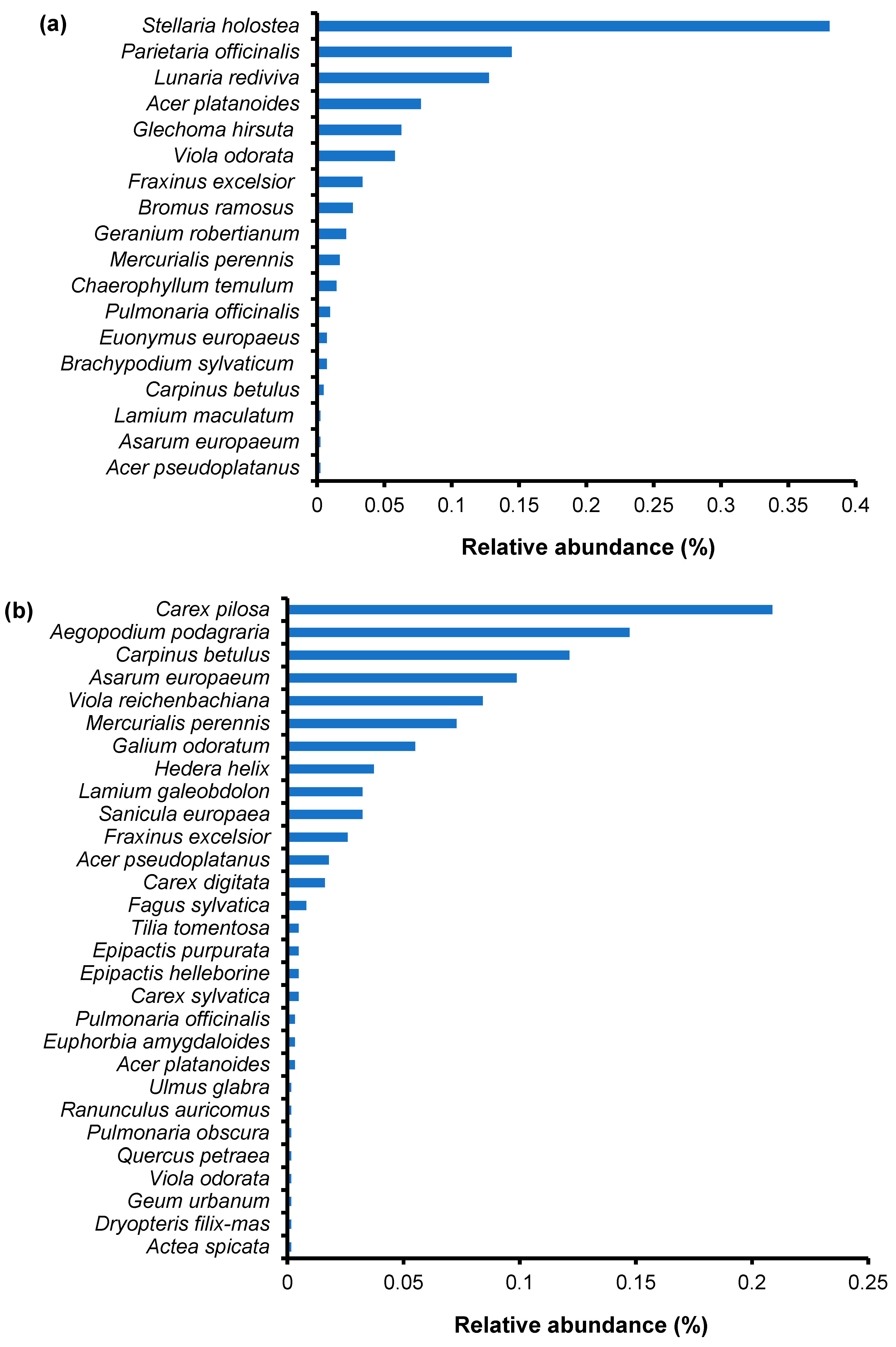
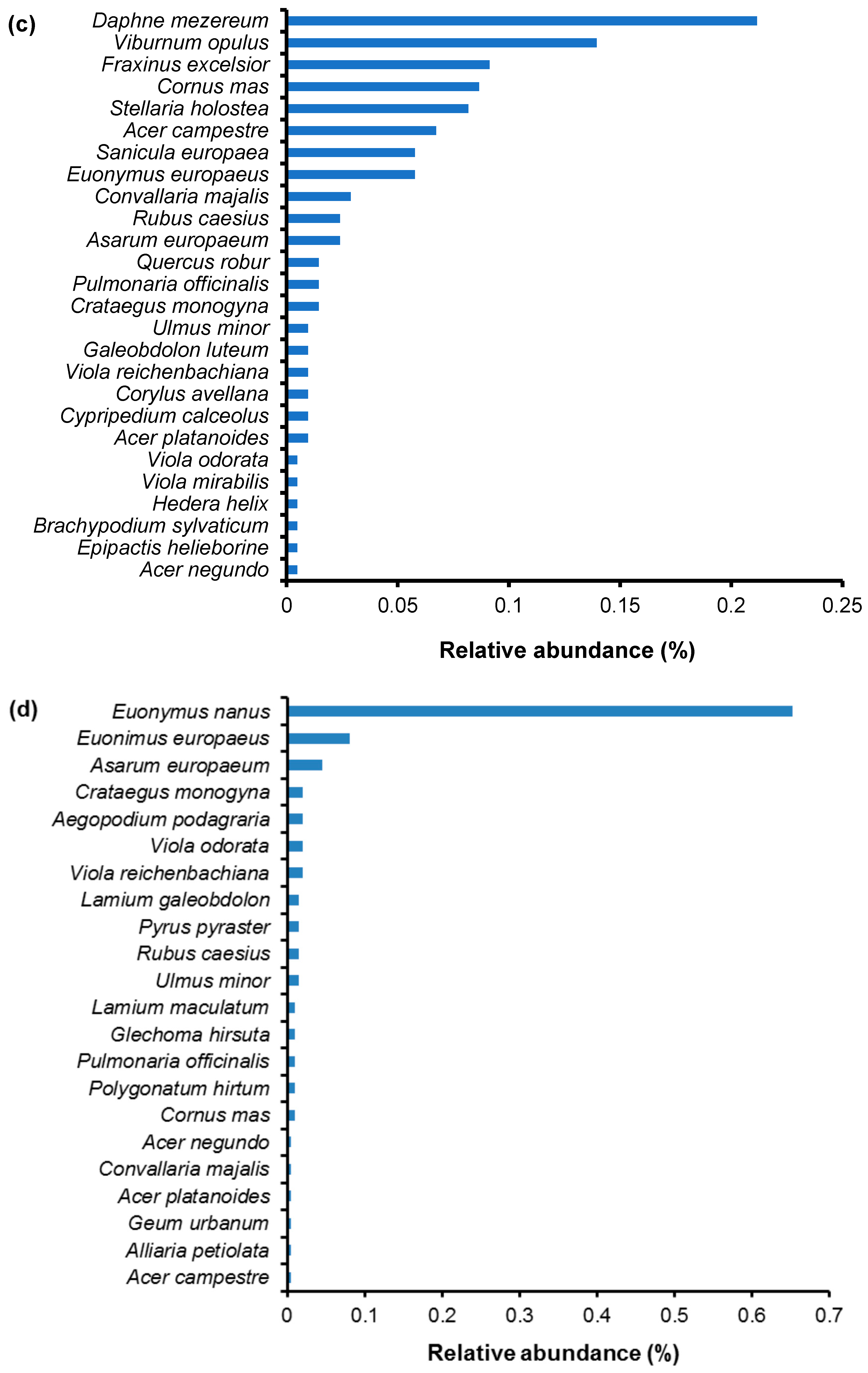
The analysis of diversity among plant communities across the four experimental plots reveals clear discrepancies in floristic composition and species abundance distribution (Figure 2a–d). According to H′, the forest communities in plots 62 and 31 exhibit moderate species richness, indicating a relatively balanced relationship between species diversity and the number of individuals. In contrast, plot 32 shows a more uneven distribution of abundance among species (H′ = 1.579), reflecting a pronounced dominance of certain species (

Table 6. Diversity indices of natural regeneration, the herbaceous vegetation layer, and shrubs at the plant community level.

Experimental Subplot	Number of Individuals (N)	Number of Species (S)	Investigated Indices
			Shannon–Wiener (H′)	Simpson (D)	Pielou (J′)	Berger–Parker (d)
15	415	18	2.055	0.198	0.711	0.381
62	620	29	2.506	0.109	0.744	0.209
31	208	26	2.636	0.101	0.809	0.212
32	199	22	1.579	0.438	0.511	0.653

).

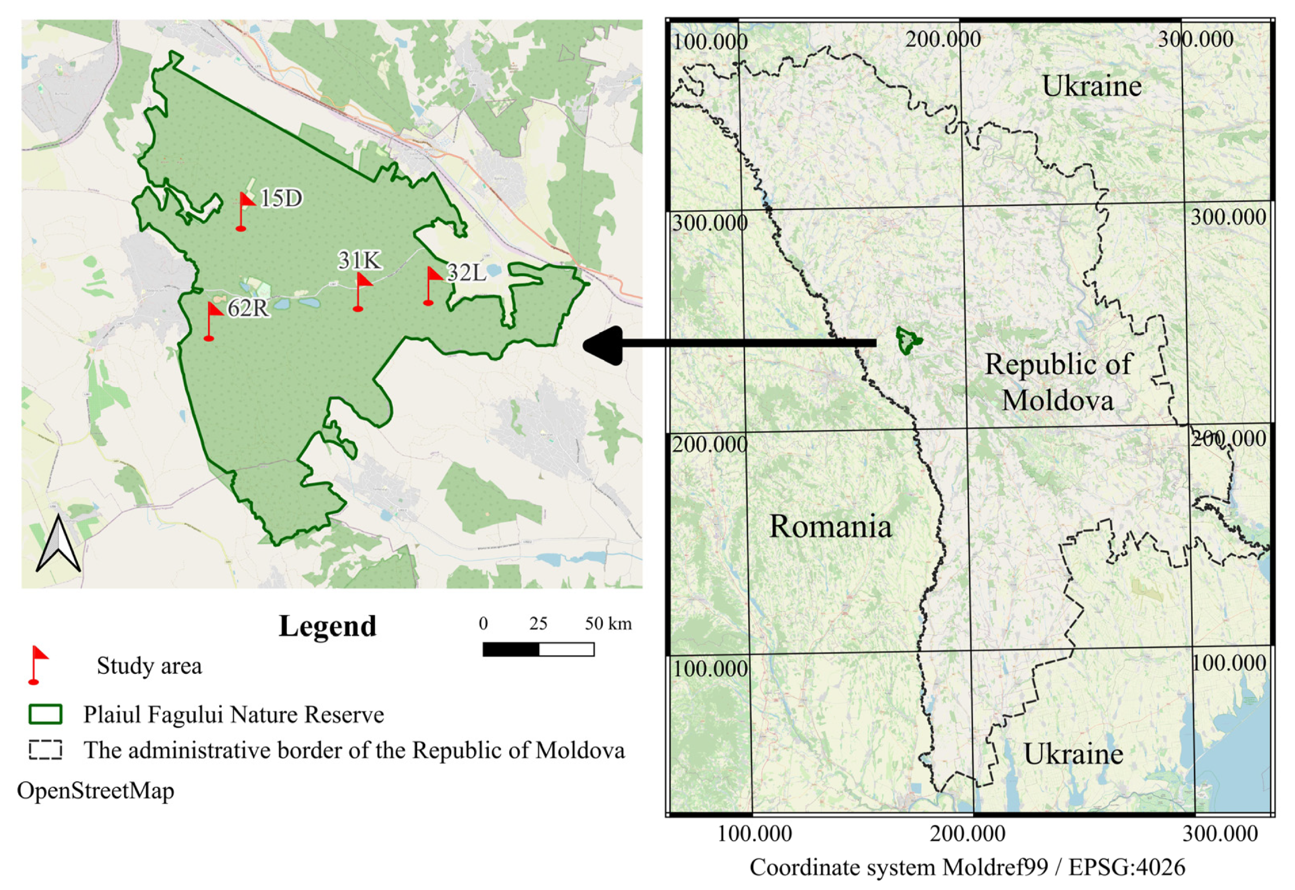
These differences can be associated with local variations in ecological conditions, such as soil type, altitude, and microtopography. The most illustrative example is plot 31, located in a ravine bottom on illuvial gray soil, which exhibits a relatively balanced species composition, compared to plot 32, situated on a north-facing slope on typical gray soil, where the dominance of certain species reduces diversity (Table 1).

According to J′, reflecting the evenness of abundance distribution among species, confirms this trend: higher values in plots 62 and 31 indicate greater uniformity, whereas the lower value in plot 32 highlights imbalance. Complementarily, d emphasizes species dominance: plots 62 and 31 show low dominance (d ≈ 0.21), while in plot 32 a single species dominates the community (Table 6).

D similarly reflects species dominance and the probability that two randomly selected individuals belong to the same species. In plot 32, D = 0.438 confirms the presence of imbalance and the strong dominance of Euonymus nanus M. Bieb. (Figure 2d), whereas the lower values of this index in plots 62 and 31 indicate more balanced and diverse communities (Table 6).

These results indicate that β-diversity among plots is influenced both by species richness and by the distribution of their abundances, suggesting that some forest communities (plot 32) are more vulnerable to diversity loss and to the dominance of a few prevailing species.

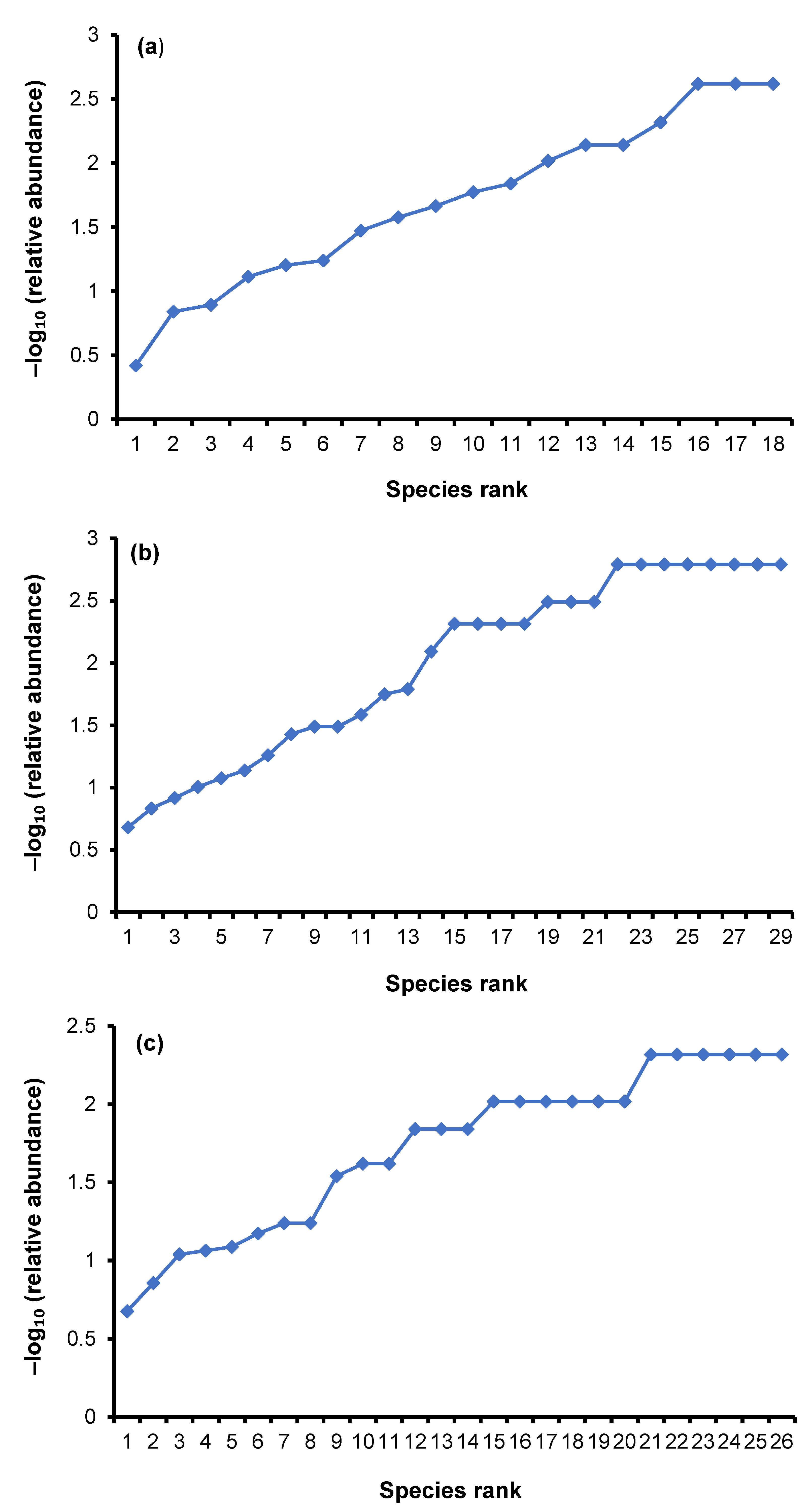
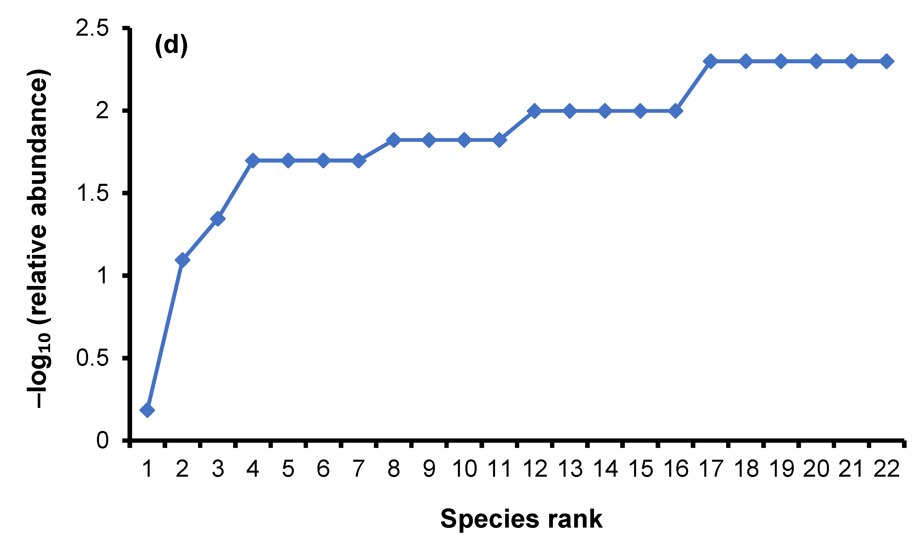
This variation in abundance distribution is clearly visualized in rank-abundance (−log₁₀(p)) plots, which highlight the internal distribution of abundances: steeper curves indicate dominant species and the presence of many rare species, while flatter curves reflect a more even distribution. This visual representation aligns with the H′ and J′ values (Table 6), demonstrating a consistent approach in evaluating differences among plots (Figure 3a–d).

The nested ANOVA indicates that species diversity (H′, D, and d) varies significantly among plots, suggesting that the structure and diversity of plant communities are influenced by the specific environmental conditions of each plot. In contrast, the evenness of species distribution (J′) does not show significant variation either among plots or among subplots, indicating that although absolute diversity differs among plots, the proportional distribution of species remains relatively constant. Additionally, differences among individual subplots are not significant, highlighting that at the local (α-diversity) level, communities are relatively homogeneous (

Table 7. Type III analysis of variance (nested ANOVA) for diversity indices.

Source of Variance	Sum of Squares	Df	Mean Square	F-Ratio	p-Value
Shannon–Wiener (H′)
A: Plot	3.689	3	1.230	13.51	p < 0.001
B: Subplot	0.857	9	0.095	1.05	p > 0.05
Residual	2.457	27	0.091
Total	7.003	39
Simpson (D)
A: Plot	0.394	3	0.131	8.23	p < 0.001
B: Subplot	0.155	9	0.017	1.08	p > 0.05
Residual	0.431	27	0.016
Total	0.981	39
Pielou (J′)
A: Plot	0.150	3	0.050	2.22	p > 0.05
B: Subplot	0.109	9	0.0121	0.54	p > 0.05
Residual	0.606	27	0.022
Total	0.865	39
Berger–Parker (d)
A: Plot	0.524	3	0.175	7.50	p < 0.001
B: Subplot	0.1540	9	0.017	0.73	p > 0.05
Residual	0.629	27	0.023
Total	1.307	39

).

The Bray–Curtis dissimilarity analysis highlights significant differences among the plant communities of the four studied plots (

Table 8. Bray–Curtis dissimilarity, turnover and nestedness components, and forest structure index among plant communities.

Plot Pairs	Bray–Curtis	Turnover	Nestedness	Forest Structure Index
15–62	0.942	0.744	0.198	0.653
15–31	0.865	0.533	0.332	0.546
15–32	0.954	0.603	0.351	0.649
62–31	0.910	0.413	0.497	0.515
62–32	0.939	0.425	0.515	0.579
31–32	0.823	0.801	0.022	0.655

). Index values range from 0.823 to 0.954, indicating a high degree of differentiation in species composition and abundance distribution among plots. Plot 32 exhibits the greatest dissimilarity relative to the other plots, with maximum dissimilarity values recorded in comparison with plots 15 and 62. This pattern reflects a distinct community structure, numerically dominated by Euonymus nanus M. Bieb., an oligodominant species in the herbaceous layer and natural regeneration stratum, likely resulting from its competitive advantage under the local edaphic and microclimatic conditions (Table 6; Figure 2d).

By contrast, the lowest dissimilarity values were observed between plots 31 and 32 and between plots 15 and 31, indicating a relatively higher similarity in terms of shared species and abundance distribution. Plot 62 occupies an intermediate position with respect to differentiation from the other plots, highlighting the presence of a mixture of dominant and subdominant species, such as Carex pilosa Scop. and Viola reichenbachiana Jord. ex Boreau, which contribute to the development of a balanced yet distinct community structure compared to the other plots (Table 8; Figure 2b and Figure 3b).

The components of dissimilarity provide insight into the ecological processes generating these differences. Turnover, representing the proportion of dissimilarity due to species replacement, with the highest values observed between plots 31–32 and 15–62. This suggests that differences among these communities primarily result from the appearance and disappearance of species characteristic of each plot. In the case of plots 31 and 32, the high turnover may be driven by successional processes in the herbaceous layer and natural regeneration, whereas for the 15–62 pair, the differences are likely influenced by habitat heterogeneity and the distinct ecological conditions in which the plant communities develop (Table 8).

Regarding nestedness, which reflects the proportion of dissimilarity due to one community being a subset of another or to abundance imbalances. High values for the 62–32 and 62–31 pairs indicate that differences are attributable to partial species presence and abundance imbalances, reflecting microhabitat heterogeneity and local selective pressures. In contrast, the 31–32 pair, with very low nestedness, demonstrates that differences are almost entirely driven by turnover, highlighting the ecological uniqueness of each community.

Values of the forest structure index ICF ranged from 0.515 for the 62–31 pair, indicating a relatively balanced and uniform structure, to 0.655 for the 31–32 pair, reflecting a more pronounced imbalance in species abundance distribution and high turnover between communities. Overall, higher ICF values were observed for the 31–32 and 15–62 pairs, indicating communities with greater internal variability and more pronounced changes in species composition, whereas the 62–31 pair exhibited the lowest index, suggesting a more stable and uniform structure. These results indicate that structural variations among plant communities are primarily determined by internal imbalance and species replacement rates, with the ICF providing an integrated measure of these aspects (Table 8).

4. Discussions

4.1. Diversity Within Subplots (α-Diversity) and Local Microhabitats

The results highlight a low to moderate α-diversity (local diversity) within the analyzed subplots, according to Shannon–Wiener index (H′) values in the Plaiul Fagului Reserve. The observed moderate level of α-diversity reflects a relatively simplified floristic structure, characteristic of stable communities dominated by a limited number of frequently occurring species. This observation can be contextualized by the findings of Maguzu et al. [24] in Kizee Village Forest Reserve, Tanzania, where H′ for tree diversity was 2.271, a value considered typical, indicating a relatively stable and ecologically balanced community.

High Pielou index (J′) values in most subplots indicate considerable structural evenness among the constituent species, suggesting low competition for resources and a balanced distribution of abundances. These features are characteristic of the herbaceous layer in mature temperate forests, where the floristic composition is dominated by stable perennial species and successional processes lead to a relative homogenization of community structure [25,26].

This combination of moderate α-diversity and high evenness reflects well-established forest ecosystems, where ecological succession has led to the stabilization of floristic composition and reduced competition among vegetation layers. Similar patterns have been reported in mature temperate forests in Central Europe, where H′ values tend to remain moderate even under conditions of high overall floristic diversity [27,28].

At the same time, the high values of the Berger–Parker (d) and Simpson (D) dominance indices observed in certain subplots, particularly those in plots 15 and 32, indicate a concentration of relative abundance towards one or a few dominant species, such as Parietaria officinalis, Stellaria holostea, and Euonymus nanus. This tendency towards oligodominance may be associated with local changes in light and moisture regimes, as well as reduced competitive pressure, favoring species adapted to specific microecological conditions [25]. Similar distributions were reported by Sitati et al. [29] in African montane forests, where certain dominant species concentrate relative abundance, reflecting oligodominant community structures.

Overall, the distribution of diversity indices among subplots suggests that the structure of the herbaceous layer and natural regeneration is primarily influenced by microhabitat heterogeneity, a phenomenon extensively documented by Ursu et al. [30] in the Plaiul Fagului Reserve. They highlighted fragmented topography and a diversity of soils, ranging from gray to brown forest soils, conditions that influence species composition and dominance. In some subplots with fresher soils, such as plot 62, species diversity is higher and the relative abundance among species is more balanced, indicating a more advanced degree of ecological stability [31]. In contrast, subplots with wetter soils, such as plot 32, dominated by Euonymus nanus, exhibit an oligodominant structure, typical of habitats influenced by floodplain conditions.

4.2. Diversity Among Plots (β-Diversity) in Forest Communities

Overall, the results indicate that variability among the experimental plots (β-diversity) follows similar trends to α-diversity. Forest plant communities are characterized by a moderate level of diversity according to H′. At the same time, evenness among species, estimated by J′, is relatively high, with the exception of plot 32, where marked dominance is observed, as reflected in the values D and d.

The diversity of forest communities is influenced by local ecological conditions, vegetation type, and the degree of ecosystem conservation. Studies from other regions indicate that differences in diversity and evenness reflect the variability of environmental conditions and the management of disturbance factors [32,33]. In such systems, plant communities are sensitive to anthropogenic interventions, and the absence of adequate management has led to reduced diversity and a simplified community structure.

A similar pattern can be observed in the Plaiul Fagului Reserve, where much of the territory is traditionally managed through regeneration cutting [34]. Our data show that species diversity (H′, D, and d) varies significantly among plots according to analysis of variance. Although silvicultural activities can exert a negative impact on the structure and composition of plant communities, the heterogeneity of habitat conditions contributes to maintaining communities with distinct structures and compositions within the reserve. This suggests that in managed ecosystems, local diversity can be conserved through the maintenance of spatial variability and a mosaic of microhabitats.

In this context, the results of J′ highlighted a moderate to high evenness in species abundance distribution among plots, with values ranging from 0.51 to 0.81. Although local variations were observed (highest evenness in plot 31 and lowest in plot 32), the differences were not statistically significant (Type III ANOVA). This indicates a relatively consistent distribution of abundance among species at the analyzed scale. Overall, these results suggest a stage of structural and functional equilibrium in the studied forest communities, reflecting the ecological stability typical of mature forests, where regeneration and competition processes reach a relatively stable level. The conclusions align with literature associating diversity and structural evenness with resilience and stability of ecosystem functions [14,31] and are supported by recent studies highlighting the role of diversity and structural organization in maintaining the spatiotemporal stability of forests [35]. Furthermore, they suggest, in agreement with Guzmán et al. [36], that seasonal structural stability, sustained by forest diversity and composition, largely explains forest ecosystem productivity and resilience. However, this interpretation should be nuanced, as the diversity–stability relationship depends on scale, community type, and the indicators used.

Our data reveal a clear dissimilarity among the studied plot communities, indicating a high degree of differentiation in species composition and abundance distribution. Certain pairs, such as 62–32 and 15–32, are dominated by characteristic species, whereas others, such as 31–32, exhibit greater similarity. Turnover and nestedness indicate that differences are driven both by species replacement and by the partial presence of other species. These findings highlight microhabitat variability and the role of local factors in maintaining diversity among plots. These results are consistent with Yu et al. [37], who reported that differences among forest communities are primarily determined by species turnover, with nestedness playing a secondary role. Similarly, a study by She et al. [38] in degraded alpine ecosystems showed that species diversity is closely correlated with community stability, with communities exhibiting higher diversity demonstrating greater stability. This suggests that microhabitat variability and differences in species composition contribute not only to dissimilarity among plots but also to the maintenance of resilience and ecological balance in the studied communities.

The values of the ICF obtained in this study (0.55–0.65) indicate a relatively balanced structure among communities. Although there is no identical composite index in the literature for direct numerical comparison, the results are conceptually consistent with studies on European deciduous forests. For example, Michalková et al. [39] showed that species composition dissimilarity (Bray–Curtis) and turnover vary moderately between inner and edge plots, depending on habitat type and the degree of fragmentation. This suggests that in unfragmented forests, differences among plots remain moderate, which is consistent with the moderate ICF values obtained in our study.

Unlike previous studies, which focused either on the analysis of a single diversity index [40,41] or on simple floristic descriptions [42], our study simultaneously integrates multiple indices and examines both local diversity (α) and diversity among plant communities (β), providing a holistic perspective on the structure of forest ecosystems. The scientific novelty lies in the application of an innovative multiparametric methodological approach, which allows the assessment of vascular species diversity at the scale of microhabitats and plot-level plant communities in a protected natural area. This approach combines diversity, evenness, and dominance indices with turnover and nestedness structures, as well as a newly introduced index, ICF. The results indicate that structural variations among plant communities are primarily driven by internal imbalance and species replacement rates, and that the ICF provides an integrated and coherent measure of these differences. The study thus proposes a replicable methodological framework, applicable to other temperate forests in protected areas, directly supporting the development of conservation measures and the maintenance of diversity and structural balance in plant communities.

Within the Plaiul Fagului Reserve, these results highlight the importance of maintaining spatial variability and a mosaic of microhabitats to conserve forest community diversity and stability. Careful management of protected forests, including controlled regeneration cuttings and monitoring of dominant species, can prevent structural simplification and support the maintenance of ecological balance. Integrating these findings into management plans therefore contributes directly to the conservation of biodiversity and the resilience of forest ecosystems.

5. Conclusions

This study presents the results of α and β diversity assessments for four experimental plots, each subdivided into 10 subplots, within the Plaiul Fagului Natural Reserve, using indices of diversity, evenness, and dominance. At the α-diversity level, plant communities in the analyzed subplots generally exhibited low to moderate diversity, with variable species abundance structures. Some subplots were dominated by a few species, whereas others showed a more balanced and complex distribution, indicating the coexistence of well-balanced microcommunities and oligodominant ones. Analysis of variance did not reveal significant differences among subplots, suggesting a relatively uniform community structure at the local scale.

At the β-diversity level, the general trend was moderate diversity for three of the plots, while plot 32 exhibited more pronounced dominance. Dissimilarity among plot-level communities was evident, and the analysis of turnover and nestedness components indicates that differences between communities are driven both by species replacement and by the partial presence of other species. The ICF values suggest a relatively balanced structure among these forest communities.

The results demonstrate that the integrated use of diversity, evenness, and dominance indices provides a robust methodological approach, applicable not only in the Plaiul Fagului Reserve but also in other similar forest ecosystems, for evaluating and comparing the diversity and structure of plant communities.