Article

Comparisons of Twelve Freshwater Mussel Bed Assemblages Quantitatively Sampled at a 15-year Interval in the Buffalo National River, Arkansas, USA

1
Department of Biological Sciences, Arkansas State University, Jonesboro, AR 72401, USA
2
Arkansas Department of Transportation, Little Rock, AR 72209, USA
3
Department of the Interior, National Park Service, Buffalo National River, Harrison, AR 72601, USA
4
Ursinus College, Collegeville, PA 19426, USA
*
Author to whom correspondence should be addressed.
Ecologies 2024, 5(1), 1-24; https://doi.org/10.3390/ecologies5010001
Submission received: 10 September 2023 / Revised: 1 December 2023 / Accepted: 11 December 2023 / Published: 23 December 2023

Abstract

:
Historically, 23 freshwater mussel species have been documented from the Buffalo National River (BNR), a 246 km, free-flowing river in northern Arkansas. The potential threats to BNR include land use/land cover changes, eutrophication, recreation, physical habitat changes, and various climate change-related effects. Twelve quantitative mussel bed sites were established and then sampled using a stratified random sampling protocol to evaluate the long-term changes between 2006 and 2020–2021 in population and assemblage characteristics. We compared (1) overall mussel bed persistence, sampling confidence levels and study-wide relative abundances, and compared species’ size and size-frequency distributions; (2) 10 overall site assemblage variables using paired t-tests; (3) site-level mean density, richness, and diversity indices using pair-wise Mann–Whitney U statistics; and (4) assemblage composition using Non-Metric Multidimensional Scaling. The major findings included the following: (1) sampling efforts based on a targeted 80% confidence level appears relatively robust, (2) BNR mussel assemblage composition and structure were relatively stable (however, small mussel bed persistence is a concern), (3) 7 of 23 sites were outliers based on freshwater mussel composition and habitat characteristics, and (4) assemblage composition changed with three species declining (Actinonaias ligamentina, Lasmigona costata, and Ptychobranchus occidentalis) and four species increasing (Cambarunio hesperus, Cyclonaias tuberculata, Eurynia dilatata, and Venustaconcha pleasii) between monitoring events.

1. Introduction

Freshwater mussels (Unionida) are some of the most imperiled taxa in the world [1,2,3], with the largest number of recent extinctions of any taxonomic group [4,5]. North America retains the greatest unionid diversity with approximately 330 recognized species; however, more than 70% are considered endangered, threatened, or of special concern [3,6,7]. Since the late 20th century, this faunal group has received a concerted effort from federal and state natural resource agencies to compile species status information [2,8,9]. Conservation efforts are hampered by our understanding of this faunal group in general and the diffuse and chronic underlying impacts that have been difficult to identify and remediate. Knowledge gaps exist in mussel systematics, life-history characteristics, fish–host relationships, and the mechanisms that drive greater sensitivity to stressors and pollutants than other organisms [1,3,10].
The most cited reasons for mussel imperilment are impoundments, invasive species, pollution, habitat destruction, and sedimentation [1,11,12,13]. Extinction gradients are observed downstream of large-scale impoundments due to altered temperature regimes, flow seasonality, food availability, and fish-host migration, which impedes the dispersal of glochidia [13]. These factors, combined with drought from global climate change, have created smaller isolated populations susceptible to genetic bottlenecks [14]. Extinction gradients are observed downstream of large-scale impoundments due to altered temperature regimes, flow seasonality, food availability, fish-host migration, and sediment deposition [13,15]. Declines in mussel abundance and species richness may permanently alter ecosystem functioning and resilience to disturbances and environmental change [16,17,18]. Long-lived organisms like unionids tend to have reduced inter-annual variation, which makes them ideal for assessing long-term ecosystem health. Identifying shifts in mussel assemblage composition and abundance over time will provide insight into the temporal scales of habitat degradation and potential environmental factors limiting population growth within a river system. Biodiversity losses and shifts in species dominance patterns include the decline in the abundance of common species [19]. Dominant mussel species are drivers of ecosystem processes and food web dynamics through their role in nutrient cycling and primary production [20]. Maintaining mussel communities will influence a cascade of ecosystem services throughout the trophic web. Few studies have documented the long-term quantitative changes in mussel communities [20,21], especially those of the “least disturbed” or minimally impacted reference sites such as designated wild and scenic or extraordinary resource waters.
The Buffalo National River (BNR) is a 246 km long, free-flowing river in northern Arkansas, which flows through the Boston Mountains and Springfield and Salem plateaus to its confluence with the White River near Buffalo City, Arkansas (Figure 1). The BNR was established as the first National River in 1972 (Public Law 92-237) and later designated as both a Wild and Scenic (for a headwaters segment; Arkansas Wild and Scenic Rivers Act of 1992) and an Extraordinary Resource Water [22,23]. However, only 11% of the BNR watershed is managed by the National Park Service (NPS) [21] and the watershed has been affected by a variety of threats [22,24,25,26,27]. In the early 1900s, BNR mussels were commercially harvested, and livestock were able to access the riverbed for stream crossing and drinking water, both of which resulted in population alteration and water quality reduction. More recently, sections of the mainstem and tributaries in the BNR watershed were 303 d listed as impaired under the Clean Water Act for bacteria and low dissolved oxygen [24], with increasing temperatures [28,29]), nutrients (in particular inorganic nitrogen), erosion/sediments, and trash identified as pollutants of concern [25]. The National Park Service [29] recently reported increased visitor use based on entry-point monitoring and anecdotal evidence of watercraft use.
Freshwater mussel assemblages in the BNR were first documented by Meek and Clark [27] in which they identified 22 species across 26 sites and reported the mussel fauna as “neither large nor plentiful” compared to that of the White River. The BNR was revisited by Harris [30] and Matthews [31], as summarized in Matthews et al. [32], and they evaluated the species composition and the physical locations of mussel assemblages. Harris [30] recorded two additional species (Pleurobema sintoxia and Eurynia dilatata) but did not observe three species (Lampsilis siliquoidea, Potamilus purpuratus, and Ligumia recta) previously listed by Meek and Clark [27]. Matthews et al. [32] expanded the survey area and distribution of freshwater mussel assemblages by approximately 33%, quantitatively sampled 23 assemblages, documented 23 species observed, and initiated a long-term monitoring program at 12 sites across three of the four upstream-to-downstream assemblage types observed in their study. Matthews et al. [32] determined 78% of the 23 species identified were state heritage ranked S1–S3 (including five of the six most abundant species) and considered the BNR a mussel diversity refuge in the Ozark Highlands. The definitions for status rank categories follow Master et al. [33]: S1, Critically Imperiled—at very high risk of extirpation in the jurisdiction due to very restricted range, very few populations or occurrences, very steep declines, severe threats, or other factors; S2, Imperiled—at high risk of extirpation in the jurisdiction due to restricted range, few populations or occurrences, steep declines, severe threats, or other factors; S3, Vulnerable—at moderate risk of extirpation in the jurisdiction due to a fairly restricted range, relatively few populations or occurrences, recent and widespread declines, threats, or other factors.
This study aimed to evaluate the changes in freshwater mussel population and community characteristics between 2006 and 2020–2021 at defined mussel assemblages (or mussel beds) in the BNR using a stratified random sampling protocol. Our first objective was to evaluate the overall characteristics of mussel bed persistence, sampling confidence levels, and study-wide relative abundances between sampling events and to compare size and size-frequency distributions of species with study-wide relative abundances ≥1%. We expected that (1) all sites would contain mussel beds, that (2) sites would be adequately sampled at ≥80% confidence levels, and that (3) study-wide species’ relative abundances, sizes, and size-frequency distributions would be similar between events. Our second objective was to compare 10 overall site assemblage variables between events using paired t-tests. We expected no significant differences in any variables between events. Our third objective was to compare site-level mean density, richness, and diversity indices between events using pair-wise Mann–Whitney U statistics. We expected no significant differences between events. Our fourth objective was to compare assemblage composition between events using Non-Metric Multidimensional Scaling. We expected sampling sites between events would cluster together, and sites would separate across an upstream-to-downstream gradient with sites in close geographic proximity clustering together.

2. Materials and Methods

2.1. Overview

Quantitative site sampling in 2006 and 2020–21 was proceeded by large-scale qualitative sampling in 2004–2005 [31] and 2019–2020 [34], respectively. After 12 monitoring sites were identified in 2006 (Table 1; Figure 1), quantitative sampling was conducted via a six-step process of qualitative reconnaissance, mussel bed delineation, mussel bed mesohabitat determination and stratification, stratified random sampling, sample processing, and in-field sampling confidence level determination with additional sampling if needed. The 2020–21 quantitative sampling followed the same methods; however, two 2006 monitoring sites no longer persisted, and three additional sites were added (Table 1).

Study Area

Stream geomorphological characteristics across the upstream to downstream gradient of sampling sites ranged from stream orders 4 to 6, drainage areas 365–3357 km2, and slopes 5.097–1.257 m/km, respectively [35]. Meanwhile, land use land cover characteristics (i.e., % development, impervious cover, and pasture land) generally increased from the upstream to downstream gradient of monitoring sites and ranged from 6.68 to 14.80% pasture, 2.38–3.38% development, and 0.14–0.27% impervious cover [35]. The entire BNR watershed mean annual precipitation is 121 cm/year [35].

2.2. Monitoring and Sampling Techniques

2.2.1. Qualitative Reconnaissance

Qualitative reconnaissance and sampling consisted of time-constrained walking visuals and snorkeling and/or diving searches that have been shown to maximize species richness determinations while remaining cost-effective [36]. Mussel assemblage sample sites were searched for no less than one person–hour, and all native mussel individuals were enumerated and identified using nomenclature of Williams et al. [37], as modified by the FMCS Common and Scientific Names subcommittee [38].

2.2.2. Mussel Bed Delineation

Field personnel located areas inhabited by mussels during qualitative reconnaissance, estimated densities and species richness, and reviewed longitudinal distribution of assemblages within the BNR prior to site selection for the mesohabitat determinations. The area inhabited (length X width) by assemblages with estimated mean densities >1 mussel/m2 (i.e., mussel beds) was determined, GPS coordinates were recorded at upstream, midsection, and downstream locations, and the bed perimeter was marked with weighted floats or survey flags/tape. Sites selected were distributed along the length of the study area.

2.2.3. Mesohabitat Determinations and Stratification

Mussel bed stratification was based on habitat characterization and the resulting mesohabitat determination was performed at each site following the Basin Area Stream Survey (BASS) protocol [39,40]. This methodology included delineating and recording each mesohabitat type (e.g., riffle, run, pool, backwater), qualitatively sampling microhabitat features such as length, width, depth, substrate, embeddedness, and instream cover, and riparian cover characteristics of bank stability and canopy coverage. We also conducted a 100-sample Wolman pebble count [41] to characterize the reach with the percentage of fine sediment, sand (fine sediment ≤ 2 mm), gravel (3–64 mm), cobble (65–256 mm), boulder (>256 mm), and bedrock. However, for the purposes of this study, we only used the microhabitat type information and associated stream length, width, and depth information for the next step of stratified random sampling.

2.2.4. Stratified Random Sampling

Sampling used simple random stratified methods [36,42]. Once assemblage areas were defined, an x, y coordinate grid was established, and quantitative sample locations were selected utilizing random number tables. If a mussel assemblage occupied diverse habitat types (i.e., riffle/pool, different substrates) or had substantially differing morphology (e.g., widths), the sampling area was stratified with each stratum sampled proportionally to area. A minimum of 10 1 m2 quadrat samples were taken at each site (unless precluded by site disturbance concerns, e.g., BR0430 in 2006), with additional quadrats added to reach an 80% confidence interval [43] for mussel density. Additionally, a 25-quadrat maximum was implemented to address substrate and mussel assemblage disturbance concerns. Sampling was performed by placing the 1 m2 quadrat at the randomly selected location with a 0.25 m2 quadrat randomly placed within. Water depth and velocity were measured in the quadrat center. Boulders and cobble were removed from the sampling area, the remaining substrate of the 0.25 m2 was extracted to a 10 cm depth and sieved to detect juvenile mussels, and the remaining portion of the 1 m2 quadrat was searched by hand to a depth of approximately 10 cm.

2.2.5. Sample Processing

All mussels encountered within the 1 m2 quadrat were bagged, brought to the surface, and identified to species [37], and updated in common data sets using FMCS [38]. The length for each mussel was measured to the nearest 0.1 mm with digital calipers. Native mussels were then replaced into the substrate from which they were taken. Voucher specimens were curated in the Arkansas State University Museum of Zoology and cataloged with the NPS. Pictures were taken of each site to document upstream and downstream reaches. Site codes were assigned using BNR standardized codes, and river kilometers (rkm) were determined from the USGS National Hydrography Dataset (NHDPlus HR) with rkm 0 at the mouth.

2.2.6. In-Field Sampling Confidence Level Determination and Additional Sampling

Sampling in 2020–21 employed predefined assemblage areas consistent with the 2006 delineations. The sampling confidence level reflected the extent to which the data accurately represented the true biodiversity characteristics of the mussel assemblage. After preliminary sampling of a minimum of 10 1-m2 quadrats, a final sample size number was determined utilizing the equation provided by Southwood [43]. The desired relative error selected for this survey was 20%. If additional samples were needed beyond the initial 10 1 m2 samples based on the estimates [43], samples were added up to a maximum of 25 total samples.

2.3. Data Analysis

Descriptive summary statistics of sampling sites’ (beds’) variables were conducted using data analysis tools in Microsoft Excel. Species richness, evenness (E), Shannon’s diversity (H’), and Simpson’s diversity (D) were calculated in PCOrd [44]. Population and community numerical standing crop estimates and 95% confidence intervals were calculated following Huebner et al. [45]. We evaluated our sampling efforts at each site and event (event X site) by estimating the relative error and the number of samples to achieve 80% and 90% confidence levels for density and species richness using methods described in Southwood [43]. To compare 2006 and 2021–21 median size and size cumulative frequency distributions of each species with study-wide relative abundance ≥1%, we used Mann–Whitney U-signed rank SigmaStats Version 4 [46] and Kolmogorov–Smirnov D tests in ExcelStats [47], respectively. To test for significant differences in bed variables between the two (2006 versus 2020–2021) sampling events, we used a paired two-tailed t-test while also testing for Shapiro–Wilk normality and estimated sample size power using SigmaStat, Version 4 [46]. Pair-wise comparisons of mean density and mean richness between sampling events of each site were assessed using SigmaStat, Version 4 [46] to conduct signed rank tests (Mann–Whitney U) due to most datasets having non-normal data based on Shapiro–Wilk tests. Finally, to evaluate if event X site communities changed between 2006 and 2020–21, we conducted a Non-Metric Multidimensional Scaling (NMS) analysis on the community-level data using PCOrd [44]. Analysis options for the NMS were set as Morisita–Horn distance measure, 500 iterations, random starting coordinates, autopilot, and a slow and thorough speed setting. We used the Morisita–Horn distance measure due to a high number of zeros in our data set and unequal sampling efforts at each site.

3. Results

3.1. An Overview of 2006 and 2020–21 Sampling Events

Of the 12 quantitative freshwater mussel assemblage long-term monitoring sites established in 2006, ten sites were sampled in 2022–21 and three (BR0256, BR0578, BR0581) additional quantitative freshwater mussel assemblage sites were established and sampled in 2020–21 (Table 1). While sites BR0350 and BR0810 were established in 2006, neither site was found in the 2020–21 sampling effort, and these two sites are believed to be extirpated. Twenty-two species were observed between the ~15-year sampling events resulting in 1878 individuals represented by 20 species sampled in 2006 and 2331 individuals represented by 17 species sampled in 2022–21 (Table 2). In 2006, the relative abundance was dominated (>1%) by 10 taxa including, in order of highest to lowest relative abundance, Ptychobranchus occidentalis, Lampsilis reeveiana, Fusconaia ozarkensis, Actinonaias ligamentina, Cambarunio hesperus, Cyclonaias tuberculata, Lasmigona costata, Venustaconcha pleasii, Pleurobema sintoxia, and Eurynia dilatata (Table 2). In 2020–21, the relative abundance was dominated by 10 taxa including, in order of highest to lowest relative abundance, P. occidentalis, C. hesperus, L. reeveiana, V. pleasii, F. ozarkensis, C. tuberculata, E. dilatata, P. sintoxia, Toxolasma lividum, and L. costata (Table 2).

3.2. Mussel Assemblage Sampling Site Variables’ Descriptions

The defined mussel bed area (m2) ranged from a low of 48 m2 to a high of 622 m2 in 2006 and a low of 48 and high of 3625 m2 in 2020–21 (Table 3). In 2006, we used 6 to 25 1 m2 quadrats to sample mussel beds, representing 4 to 10% of the defined mussel bed area. Meanwhile, in 2020–21, we used 10 to 25 1 m2 quadrats to sample the mussel beds, representing 1 to 21% of the defined mussel bed. The mean density ranged from 1.3 to 22.6 individuals/m2 in 2006 and from 2.4 to 23.5 individuals/m2 in 2020–21. The community numerical standing crop ranged from 213 (±124) to 14,801 (±2227) individuals in 2006 and from 298 (±127) to 83,558 (±15,369) individuals in 2020–21. The total richness ranged from 4 to 16 in 2006 and from 5 to 12 in 2020–21. The number of S1, S2, and S3 richness ranged from three to six in 2006 and from three to seven in 2020–21. Furthermore, the combined S1, S2, and S3 relative abundance ranged from 39.5 to 93.4% in 2006 and from 33.8 to 95.7% in 2020–21. The mussel bed assemblage evenness ranged from 0.560 to 0.894 in 2006 and from 0.363 to 0.875 in 2020–21. Shannon’s diversity (H’) ranged from 0.892 to 2.260 in 2006 and from 0.651 to 2.015 in 2020–21. Simpson’s diversity (D) ranged from a low of 0.4930 to a high of 0.8741 in 2006 and from a low of 0.2758 to a high of 0.8423 in 2020–21. In 2006, the number of species with only one occurrence at a site (singlet) ranged from zero to five, while the number of species with only two occurrences at a site (doublet) ranged from zero to three. Meanwhile, the number of species with only one occurrence at a site (singlet) ranged from one to five while the number of species with only two occurrences at a site (doublet) ranged from zero to two in 2020–21.

3.3. Sampling Confidence Levels of 2006 and 2020–21

In 2006, the sample size confidence level based on density ranged from 57.2 to 91.1 with 9 of 12 sampling efforts meeting the 80% confidence level target, and the confidence level based on richness ranged from 72.2 to 96.4 with 9 of 12 sampling efforts meeting 80% (Table 4). Meanwhile, the 2020–21 sample size confidence level based on density ranged from 67.5 to 91.6 with 9 of 13 sampling efforts meeting the 80% confidence level, and the confidence level based on richness ranged from 75.6 to 94.3 with 11 of 13 sampling efforts meeting 80% (Table 4). For both sampling density and richness, we provided the number of samples needed to reach 80 and 90% confidence levels to compare the required efforts (Table 4).

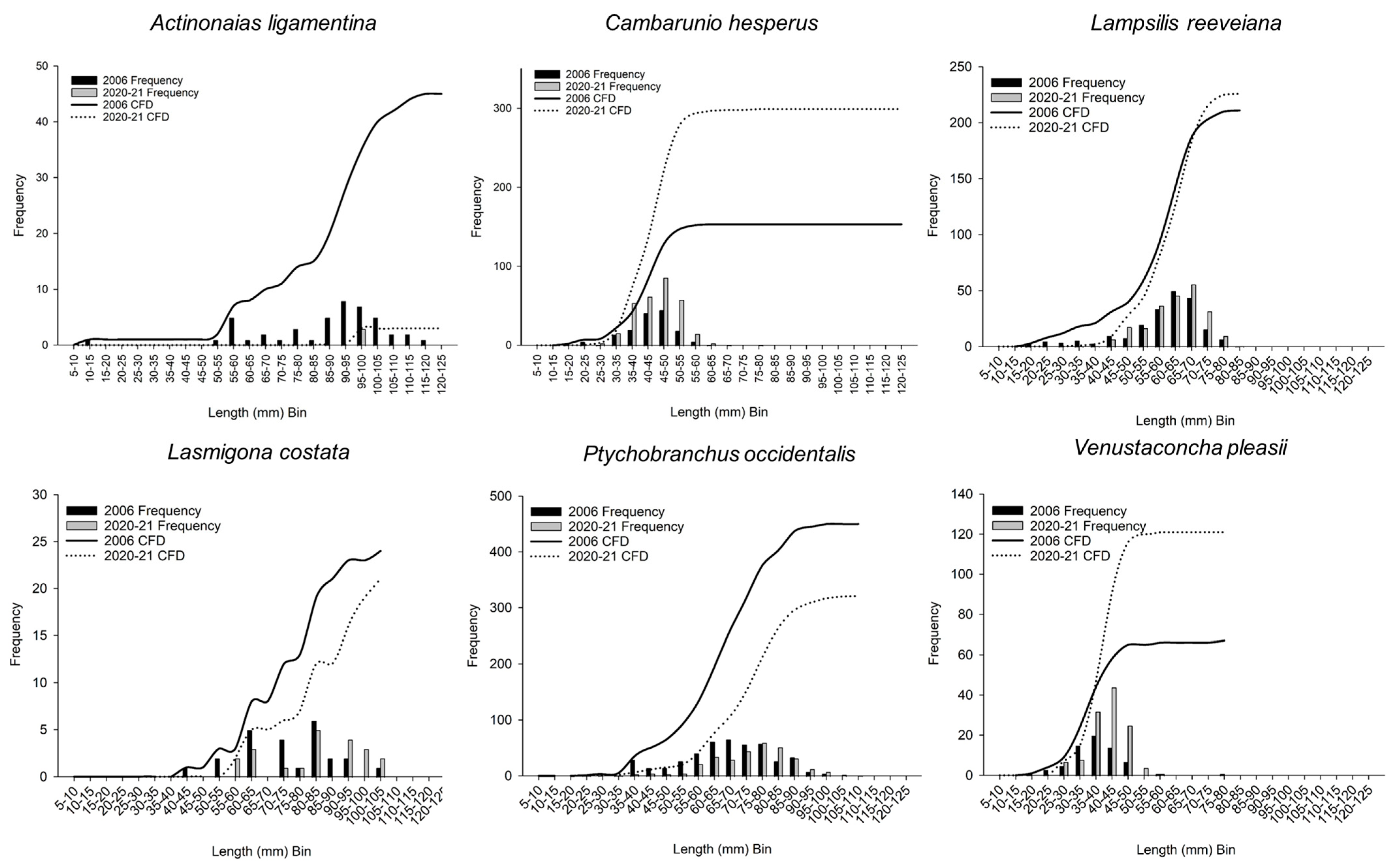
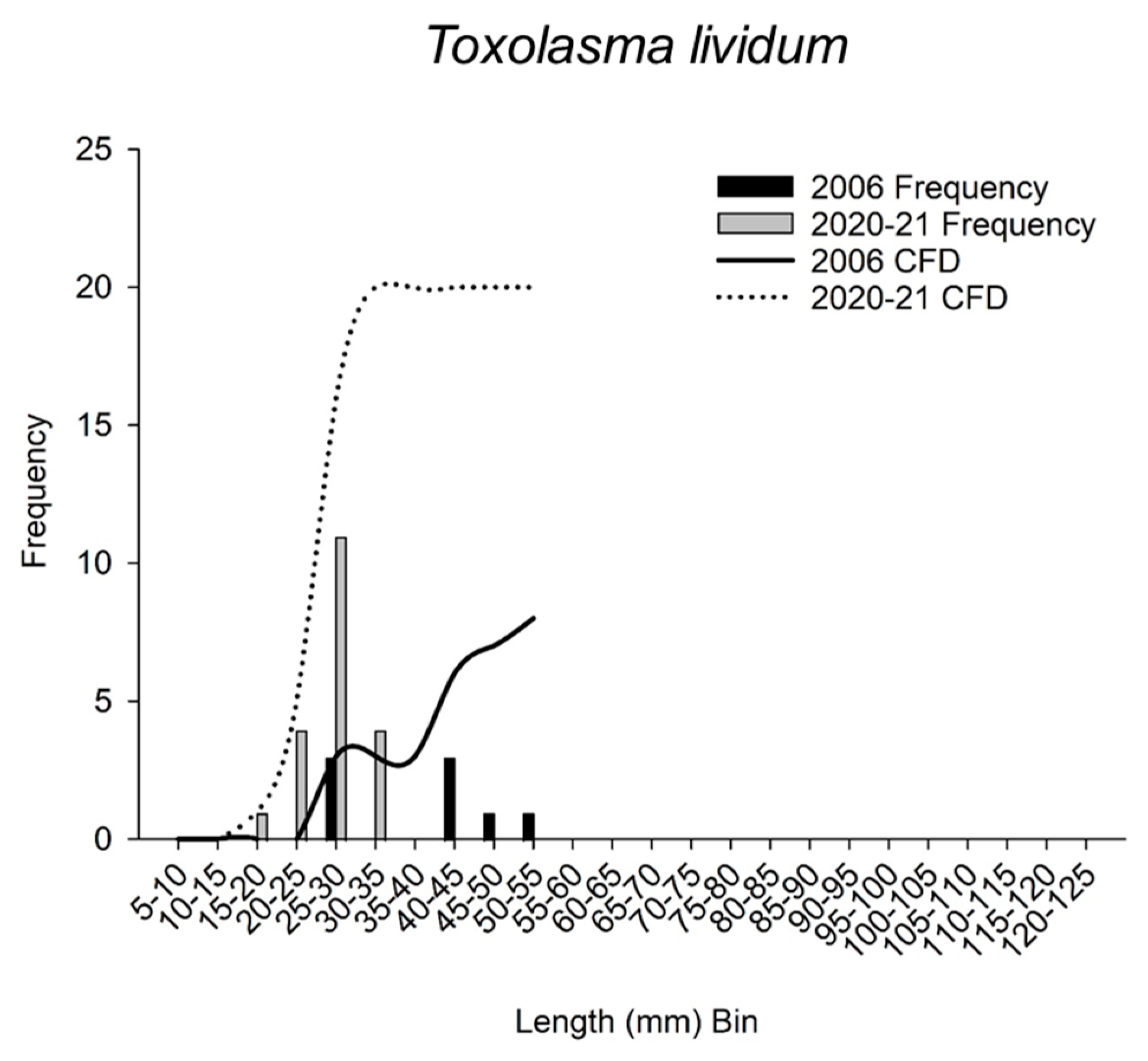
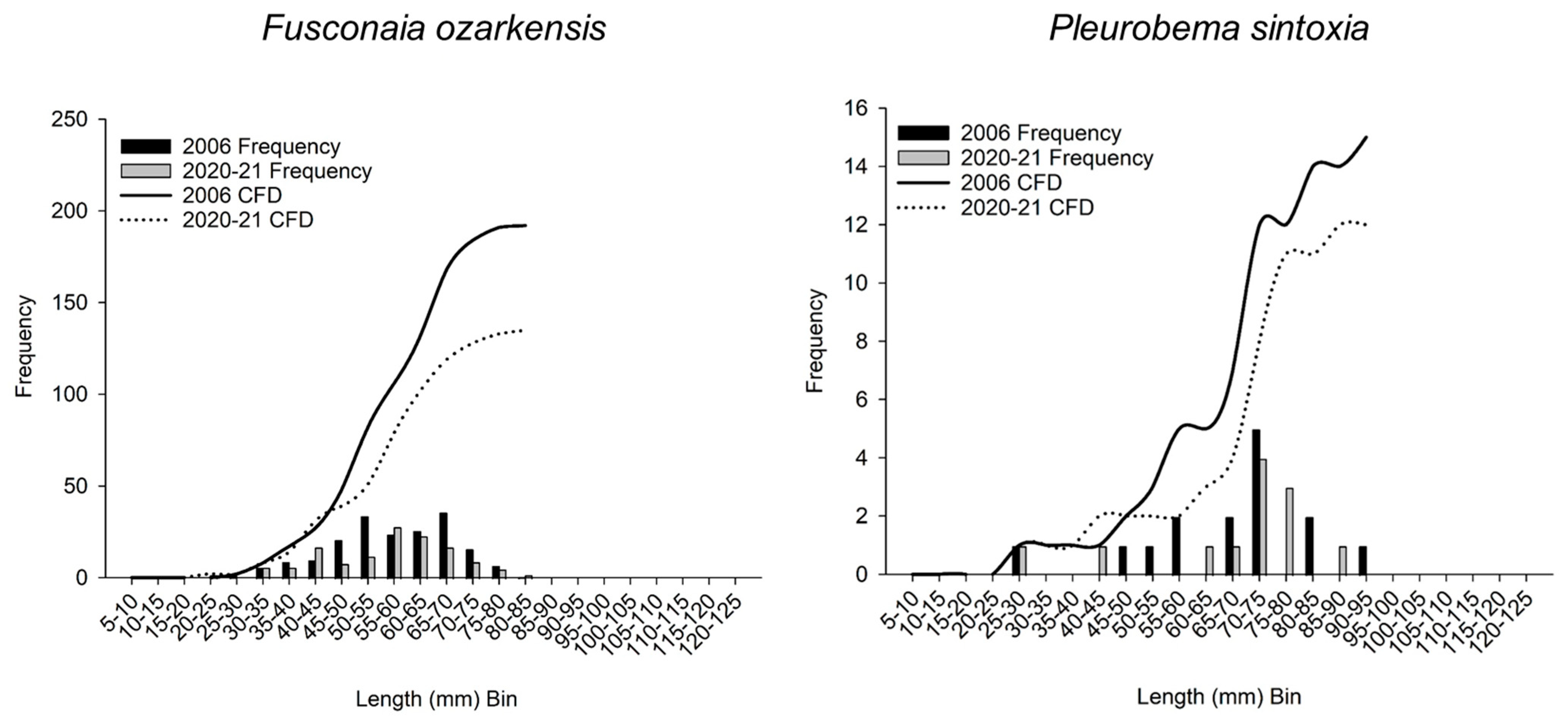
3.4. Size and Cumulative Frequency Distributions

Mann–Whitney U pairwise comparisons between 2006 and 2020–21 median lengths for 11 species resulted in seven statistically significant comparisons with six showing significantly a higher length in 2020–21 samples (Table 5). Pair-wise Kolmogorov–Smirnov length cumulative frequency distribution analysis resulted in nine significantly different pair-wise comparisons (Table 5). Six species (A. ligamentina, C. hesperus, L. reeveiana, L. costata, P. occidentalis, and V. pleasii) showed significantly different distributions with low to no recruitment (Table 5; Figure 2). Two species (C. tuberculata and E. dilatata) showed significantly different distributions with different recruitment patterns between 2006 and 2020–21 (Table 5; Figure 3). Toxolasma lividum showed significantly different distributions with higher recruitment but fewer larger individuals in 2020–21 (Table 5; Figure 4). Meanwhile, two species (F. ozarkensis and P. sintoxia) showed similar distributions between the two sampling events (Table 5; Figure 5).

3.5. The Paired t-Test of Common 2006 and 2020–21 Sites

We conducted 10 paired t-test comparisons for 10 overall variables (Table 3) associated with the common 2006 and 2020–21 sampling sites, and all 10 datasets had normal distributions based on Shapiro–Wilk Normality (p ≤ 0.05); however, almost all datasets had low statistical power (Table 6). While none of the paired t-test comparisons were statistically significant, four variable means were higher (sample size, % bed sampled, S1–S3 richness, and S1–S3 abundance) and six variable means were lower (density, total richness, evenness, Shannon’s diversity, Simpson’s diversity, and number of singlets and doublets) in the 2020–21 monitoring efforts.

3.6. The Pairwise Density and Richness Comparisons of 2006 and 2020–21

For the 10 commonly sampled sites, we conducted pairwise comparisons for sampling density and richness using the non-parametric Mann–Whitney U statistic because most of our datasets were found to have non-normal distributions based on Shapiro–Wilk Normality (p ≤ 0.05). Of the 20 pair-wise comparisons, only 6 comparisons were statistically significant (Table 7). The 2020–21 sampling was found to be significantly lower for BR0260 richness, BR0626 density and richness, and BR0820 density and richness but was statistically higher for BR0579 density (Table 7). Unlike the paired t-test comparisons, no general non-significant trends in higher or lower density and richness were observed between the two sampling events.

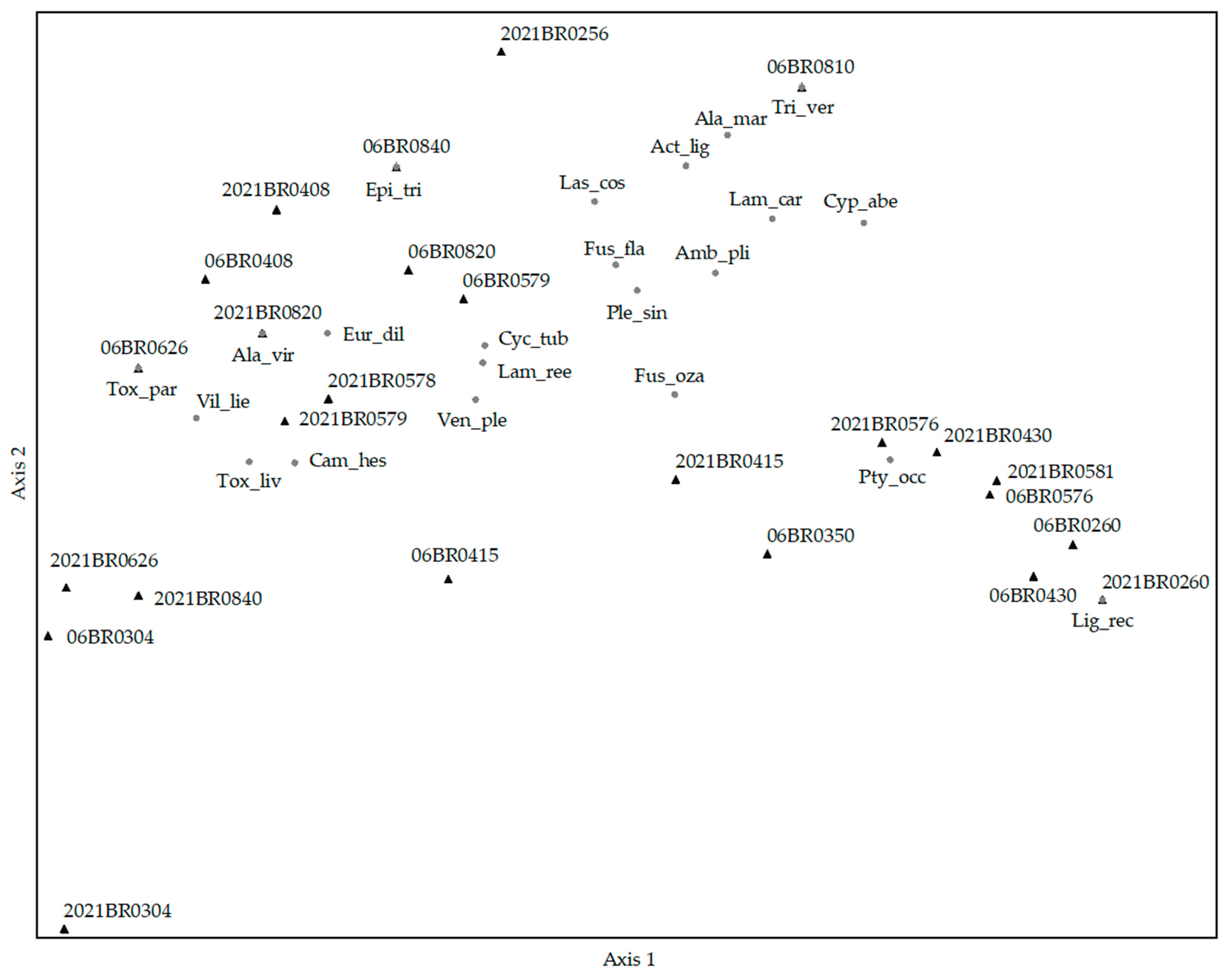
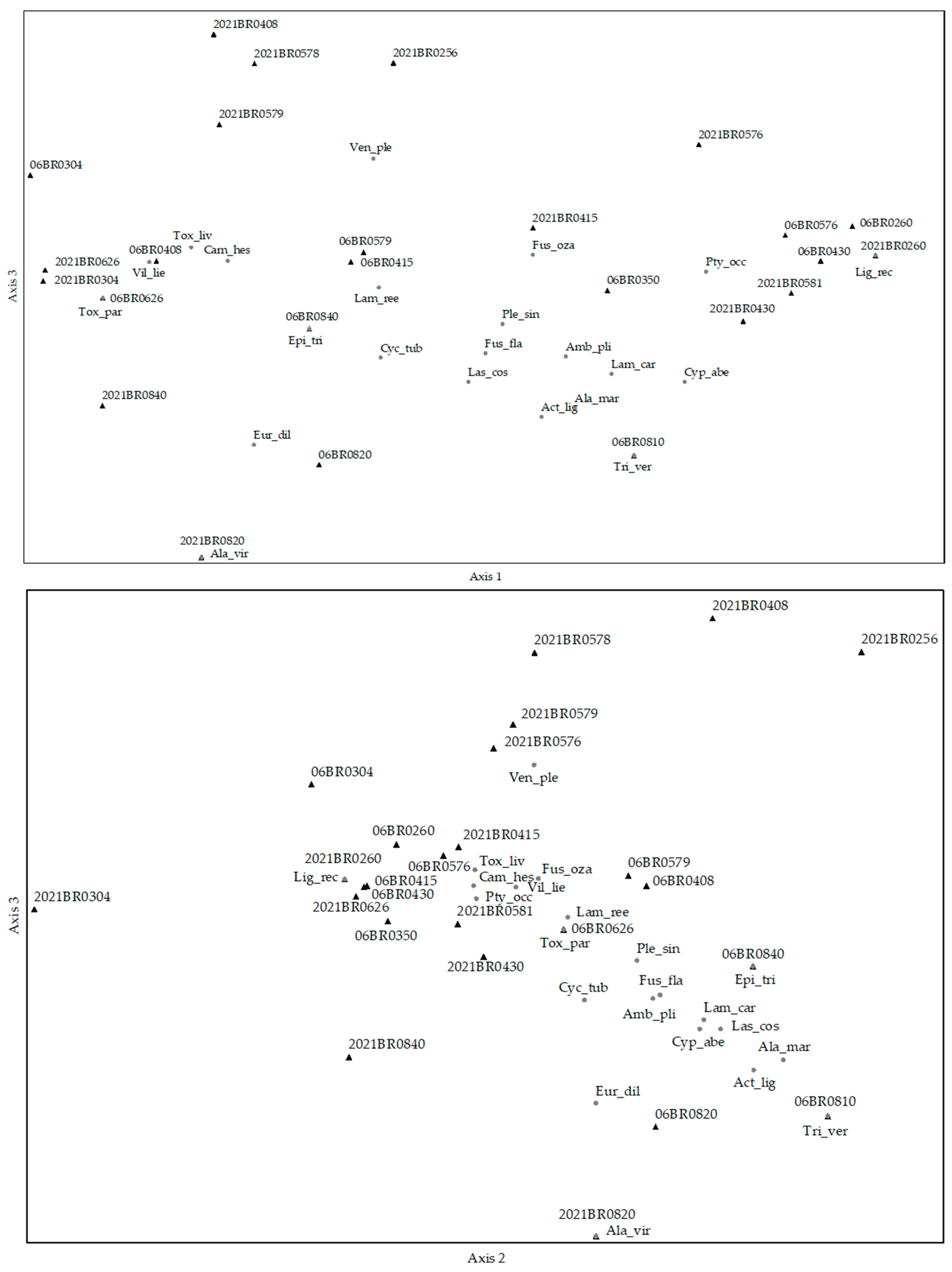
3.7. The Assemblage Comparisons of 2006 and 2020–21

Our NMS of 25 event X site combinations with 22 species abundances resulted in a recommended 3-dimensional solution with a final stress of 6.16652, a final instability of 0.00000, 71 iterations, R*n (nonmetric fit) of 0.9962, R*l (linear fit) of 0.9779, and R*m (metric fit) of 0.9649. Contrary to our expectations, there was little upstream-to-downstream spatial clustering of sites along axes’ 1–3 coordinate scores; however, the downstream sites (BR800s) were distributed at higher values of Axis 2 and lower values of Axis 3 (Figure 6). Furthermore, only a few event x site samples were outliers, such as 06BR0810 (higher on Axis 2), 2021BR0256 (higher on Axis 2 and 3), 2021BR0304 (lower on axes 1 and 2), and 2021BR0408 (high on axes 1 and 3) (Figure 6). Meanwhile, the distribution of NMS ordination scores resulted in modest temporal variation between 2006 and 2021 sampling events (Figure 6), contrary to our expectations of event X site clustering closely together, indicating similar assemblages through time. There were six species positively correlated (C. aberti, F. ozarkensis, L. cardium, L. recta, P. occidentalis, and V. pleasii) and four species negatively correlated (C. hesperus, L. costata, T. lividum, and L. lienosus) with Axis 1 (Table 8). There were fourteen species positively correlated (A. ligamentina, A. marginata, C. turberculata, E. dilatata, E. triquetra, F. flava, F. ozarkensis, L. cardium, L. reeveiana, L. costata, P. sintoxia, T. verrucosa, and V. pleasii), but there was only one species negatively correlated (L. recta) with Axis 2 (Table 8). There was one species positively correlated (V. pleasii), but there were eight species negatively correlated (A. ligamentina, A. plicata, C. tuberculata, E. dilatata, F. flava, L. costata, and T. verrucosa) with Axis 3 (Table 8).

4. Discussion

4.1. Overview

We identified four major findings while comparing our 2006 and 2020–21 BNR monitoring sites. First, our sampling protocol to achieve a targeted 80% confidence level appeared to be relatively robust, but additional samples were required in some cases. Second, BNR mussel assemblage compositions and structures were relatively stable through the ~15-year sampling window; however, there are concerns for mussel bed persistence due to ~17% loss of sampled beds. Third, in addition to two 2006 sampling sites no longer persisting in 2020–21, seven of the remaining twenty-three sites were outliers based on their freshwater mussel composition and characteristics. Finally, based on both relative abundance and the NMS, assemblage composition had changed with three abundant species declining (A. ligamentina, L. costata, and P. occidentalis), and four species increasing (C. hesperus, C. tuberculata, E. dilatata, and V. pleasii) between sampling events.

4.2. Sampling Effort

To provide guidance for gathering statuses and monitoring information on freshwater mussels, Smith and Strayer [36] proposed adopting standardized sampling designs and methods based on the needs of the study. For the BNR, we used a stratified random sampling design which has been commonly used for surveying mussels in Arkansas rivers since the early 1990s [31,48,49,50,51,52,53]. Overall, our sampling efforts during both monitoring events were robust, with 18 of 25 event X site sampling efforts achieving 80% or higher confidence levels for site mean density and 20 of 25 event X site sampling efforts achieving 80% or higher confidence levels for site mean richness. The 80% confidence level for sample density and richness provided valuable information on the status of freshwater mussels, sufficient to inform management decisions at a reasonable expense. For example, achieving 90% confidence levels for both density and richness would require doubling the sample efforts in most cases. These sampling efforts and confidence level results are consistent with other studies that used similar sampling designs across small to large streams [42,52].

4.3. Species and Assemblage Composition and Structure Changes

The paired t-tests of 10 variables comparing 2006 and 2020–21 sampling efforts for 10 common sites showed no significant differences. Only 6 of 20 Mann–Whitney U tests comparing the mean density and richness of 2006 versus 2020–21 sites were statistically different. However, in addition to 5 of 6 Mann–Whitney U tests indicating that 2020–21 richness or density was significantly lower than 2006 samples, most assemblage structure variables in the paired t-test were lower in 2020–21, though not statistically significant. The exceptions were that sample size, % bed sampled, S1-S3 richness, and S1-S3 abundance were slightly higher in 2020–21 than in 2006. Furthermore, among the dominant taxa (>1% relative abundance), five taxa declined, four taxa increased, and one species stayed the same in relative abundance between 2006 and 2020–21. Declining relative abundance taxa included A. ligamentina, F. ozarkensis, L. costata, P. sintoxia, and P. occidentalis, with A. ligamentina decreasing from 9.3 to 0.3% and P. occidentalis decreasing from 31.2 to 22.5%. Meanwhile, A. ligamentina, L. costata, and P. occidentalis also showed statistically different size-frequency distributions with lower recruitment. Conversely, the increasing relative abundance of dominant taxa included C. hesperus, C. tuberculata, E. dilatata, and V. pleasii. In contrast, C. hesperus and V. pleasii size-frequency distributions indicated different size frequency distributions between sampling events with lower recruitment in the 2020–21 samples while C. tuberculata and E. dilatata showed different distributions with different recruitment frequencies between sampling events. Cambarunio hesperus increased from 8.8 to 18.3%, C. tuberculata increased from 5.8 to 9.2%, E. dilatata increased from 1.5 to 4.5%, and V. pleasii increased from 3.9 to 13.5%. Furthermore, L. reeveiana maintained its relative abundance at 15.1% between the ~15-year sampling events. In terms of species observations, five species were observed in 2006 (C. aberti, E. triquetra, F. flava, T. verrucosa, and T. parvum) but not in 2020–21, while two species were observed in 2020–21 (A. viridis and L. recta), but not in 2006. In all cases, these observations were low (<11) with A. viridis, C. aberti, E. triquetra, L. recta, and T. verrucosa all represented by one–three individuals. The 2006 E. triquetra record was from one individual and could have been a misidentified A. viridis [54].
Stream size and life history strategies influence the occurrence and distribution of North American freshwater mussels [55]. Haag [55] identified dominant (10% or more of the relative abundance) mussel species across small, medium-sized, and large Mississippian region streams. Three life history strategies have been proposed for North American freshwater mussels that include opportunistic (disturbed and unstable but productive habitats), periodic (unproductive or high variability/stress habitats), and equilibrium (stable, productive habitats) strategies. Species that declined between 2006 and 2020–21 were mostly equilibrium-strategy species (A. ligamentina, F. ozarkensis, P. sintoxia, and P. occidentalis) that are known to inhabit mid-sized streams, while L. costata is considered a periodic strategist that mostly inhabits small streams and to a lesser extent mid-sized streams. Two of the four species that increased between 2006 and 2021–22 do not have a clear characterized life history strategy (C. tuberculata and E. dilatata) but C. hesperus is an opportunistic strategist that inhabits mostly small streams and V. pleasii can be classified as a periodic-strategy species and is not known as a dominant species in any stream size category. For the rare species observed (C. aberti, E. triquetra, F. flava, T. verrucosa, and T. parvum), none were expected to be dominant (>10% relative abundance) small, medium, or large river species except for F. flava, but they represented each life history strategy: opportunistic (T. parvum), periodic (E. triquetra), equilibrium (C. aberti, F. flava, T. verrucosa).
This suggests that while there have been small changes, mostly declines, in assemblage characteristics such as diversity metrics, there have been modest to large changes in recruitment and assemblage composition in BNR mussels. While some of these compositional changes may be attributed to the small number differences in sampling sites between the ~15-year sampling events, the nearly 10% relative abundance declines of A. ligamentina (G5 and S4) and P. occidentalis (G3/G4 and S3) are noteworthy, as are the nearly 10% relative abundance increases of C. hesperus (G5 and S3) and V. pleasii (G3/G4 and S3). For those taxa that declined between the ~15-year sampling events, it is possible that stream conditions have become less stable than in the past. For example, both A. ligamentina and P. occidentalis have been reported to be thermally and drought sensitive [56,57]. Given that rising temperature is a growing concern in the BNR [26,28], increases in the magnitude, duration, and frequency of these events pose major risk to long-lived species. Meanwhile, for the species that increased in relative abundance, they are classified as non-equilibrium-strategy species that are better suited to higher disturbance and stress. These overall relative abundance changes, plus the observation that S1–S3 richness and relative abundance increased from 2006 to 2020–21, suggest that freshwater mussel assemblage changes are occurring in the BNR. These changes warrant further monitoring of mussel assemblages and environmental variables (e.g., geomorphological channel shifts and erosion, nutrients, climate and land use land cover change). Continued habitat monitoring within mussel bed areas in conjunction with quantitative sampling events may provide more insight on these shifts in composition.

4.4. Mussel Bed Persistence and Outliers

Between the two sampling events, we sampled 25 event X site combinations with 10 common sites across the ~15-year interval. In 2020–21, we added three additional long-term quantitative monitoring sites with BR0256 added to the upstream extent of monitoring and BR0578 and BR0581 added due to their bed size, density, and richness. Sites BR0350 and BR0810 were established in 2006, but neither site was located during the 2020–21 sampling effort, and these two sites are no longer believed to be extant. The loss of these two mussel bed sites across the 15-year sampling interval represents a 17% loss of sampled mussel beds. Anecdotal observations at BR0350 and BR0810 suggest substantial geomorphological changes occurred in the ~15-year time interval. The BNR is a relatively high gradient stream system (with steeper gradients and rapid elevation changes in the upper reaches in the Boston Mountains) and channel-changing flood events are known to occur [31]. Discharge measurements at USGS monitoring stations revealed two moderate flood stages (<10.7 m) and three minor flood events (<8.2 m) occurred between sampling events and satellite imagery at each site documented channel changes. Across the two mussel bed sites along the BNR, varying flood-event intensities may have collectively degraded the habitat, rendering it unsuitable due to physical disruption, sediment accumulation, bank erosion, water quality fluctuations, and food availability. Dedicated monitoring such as the current study paired with side-scan sonar surveys can document mussel bed persistence and habitat stability in the BNR.
For our NMS analysis, we expected that event X site samples would show an upstream-to-downstream distribution gradient with spatial and temporal assemblage similarities. However, aside from the downstream sites (BR800s) being distributed at higher values of Axis 2 and lower values of Axis 3, there was little evidence of an upstream-to-downstream distribution for our NMS analysis. In retrospect, because our sampling sites were distributed within the fourth to sixth stream order section of the Buffalo River, our pattern is consistent with patterns observed by Haag [55] in which certain genera and species are known to differentially inhabit small, medium, or large streams where our BNR sampling occurred withing Haag’s “medium sized streams” assemblage structure. Furthermore, our NMS analysis resulted in four event x site samples (i.e., 06BR0810, 2021BR0256, 2021BR0304 and 2021BR0408) being outliers. The 06BR0810 was characterized by high numbers or the presence of A. ligamentina, A. marginata, A. plicata, C. aberti, F. flava, F. ozarkensis, L. costata, L. cardium, L. reeveiana, P. sintoxia, and P. occidentalis, and was the only site to include T. verrucosa. It should also be noted that the 06BR0810 mussel assemblage (i.e., bed) was one of two sites that was not found in the 2020–21 sampling event and is most likely extirpated given no mussels were found. The 2021BR0256 assemblage was influenced by only having five species present (F. ozarkensis, L. cardium, L. reeveiana, L. costata, and P. occidentalis), which were low in abundance, and none of which were unique to 2021BR0256. The 2021BR034 assemblage was influenced by being represented by only six species with C. hesperus dominating (n = 50) the abundance while the other four species had abundances of one–three individuals. The 2021BR0408 assemblage was influenced by relatively low abundances of 10 commonly sampled BNR species.

5. Conclusions

While our analysis suggests that BNR mussels were relatively stable between the 15-year sampling interval, mussel bed persistence and trends in population and assemblage characteristics warrant continued monitoring. Investigation into areas such as hydrodynamic modeling, changes in fish host communities, and dissolved oxygen and pollutant load dynamics should be considered. With only a relatively small portion of the BNR watershed managed by the NPS, a catchment approach related to tributaries feeding into the mainstem may be necessary to include in a monitoring plan that will involve multiple entities such as local stakeholders and state agencies. Long-term quantitative studies of mussel assemblages paired with monitoring environmental drivers in the BNR are essential in documenting changes and providing timely data points for conservation and management decisions.

Author Contributions

Conceptualization, J.L.H., S.W.H. and A.D.C.; methodology, J.L.H. and A.D.C.; software, A.D.C.; validation, A.M.P., M.W.M., J.L.H. and A.D.C.; formal analysis, A.M.P., M.W.M., J.L.H. and A.D.C.; investigation, A.M.P., M.W.M., S.W.H., A.R.R., J.L.H. and A.D.C.; resources, S.W.H., J.L.H., J.L.B. and A.D.C.; data curation, A.M.P., M.W.M., J.L.H. and A.D.C.; writing—original draft preparation, A.M.P. and M.W.M.; writing—review and editing, A.M.P., M.W.M., S.W.H., A.R.R., J.L.B., J.L.H. and A.D.C.; visualization, M.W.M., A.M.P. and A.D.C.; supervision, S.W.H., J.L.H., J.L.B. and A.D.C.; project administration, S.W.H., J.L.B., J.L.H. and A.D.C.; funding acquisition, A.D.C., J.L.B. and J.L.H. All authors have read and agreed to the published version of the manuscript.

Funding

This research was funded by the Department of Interior, National Park Service, with contracts with Arkansas State University with A.D.C and J.L.B and J.L.H being the custodians.

Institutional Review Board Statement

Not applicable.

Informed Consent Statement

Not applicable.

Data Availability Statement

Data associated with this publication is published in Harvard Dataverse (view at https://dataverse.harvard.edu/dataverse/harvard) listed as “Buffalo River Quantitative Mussels 2005–2021 and can be viewed at https://dataverse.harvard.edu/dataset.xhtml?persistentId=doi:10.7910/DVN/JZPHXS.

Acknowledgments

Field and laboratory assistance in 2004–2006 was provided by: R. Allen, T. Bianco, D. Hayes, K. Inoue, R. Lawson, H. Martin, A. Peck, H. Thomas, F. Usrey, N. Wentz, and J. Yancy. Field and laboratory assistance in 2019–2021 was provided by: D. Filipek, H. Hall, J. Kunz, J. Steevens, M. Trenchik, and L. Yates.

Conflicts of Interest

The authors declare no conflicts of interest. While several of the authors (S.E. Hodges and A.R. Rodman) are/were employees of the Buffalo National River at the time of the study, the Buffalo National River and Department of Interior organization had no role in the design of the study; in the collection, analyses, or interpretation of data; in the writing of the manuscript; or in the decision to publish the results as an administrative entity.

References

  1. Haag, W.R.; Williams, J.D. Biodiversity on the Brink: An Assessment of Conservation Strategies for North American Freshwater Mussels. Hydrobiologia 2014, 735, 45–60. [Google Scholar] [CrossRef]
  2. Lopes-Lima, M.; Burlakova, L.E.; Karatayev, A.Y.; Mehler, K.; Seddon, M.; Sousa, R. Conservation of Freshwater Bivalves at the Global Scale: Diversity, Threats and Research Needs. Hydrobiologia 2018, 810, 1–14. [Google Scholar] [CrossRef]
  3. Strayer, D.L.; Downing, J.A.; Haag, W.R.; King, T.L.; Layzer, J.B.; Newton, T.J.; Nichols, S.J. Changing Perspectives on Pearly Mussels, North America’s Most Imperiled Animals. Bioscience 2004, 54, 429–439. [Google Scholar] [CrossRef]
  4. Lydeard, C.; Cowie, R.H.; Ponder, W.F.; Bogan, A.E.; Bouchet, P.; Clark, S.A.; Cummings, K.S.; Frest, T.J.; Gargominy, O.; Herbert, D.G.; et al. The Global Decline of Nonmarine Mollusks. BioScience 2004, 54, 321–330. [Google Scholar] [CrossRef]
  5. Régnier, C.; Fontaine, B.; Bouchet, P. Not Knowing, Not Recording, Not Listing: Numerous Unnoticed Mollusk Extinctions. Conserv. Biol. 2009, 23, 1214–1221. [Google Scholar] [CrossRef] [PubMed]
  6. Bogan, A.E. Freshwater Bivalve Extinctions (Mollusca: Unionidae): A Search for Causes. Am. Zool. 1993, 33, 599–609. [Google Scholar] [CrossRef]
  7. Williams, J.D.; Warren, M.L.; Cummings, K.S.; Harris, J.L.; Neves, R.J. Conservation Status of Freshwater Mussels of the United States and Canada. Fisheries 1993, 18, 6–22. [Google Scholar] [CrossRef]
  8. Freshwater Mollusk Conservation Society. A National Strategy for the Conservation of Native Freshwater Mollusks. Freshw. Mollusk Biol. Conserv. 2016, 19, 1–21. [Google Scholar] [CrossRef]
  9. Neves, R.J.; Bogan, A.E.; Williams, J.D.; Ahlstedt, S.A.; Hartfield, P.W. Status of Aquatic Mollusks in the Southeastern United States: A Downward Spiral of Diversity. In Aquatic Fauna in Peril: The Southeastern Perspective; Benz, G.W., Collins, D.E., Eds.; Special Publication 1; Southeast Aquatic Research Institute, Lenz Design & Communications: Decatur, GA, USA, 1997; pp. 43–86. [Google Scholar]
  10. Campbell, D.C.; Serb, J.M.; Buhay, J.E.; Roe, K.J.; Minton, R.L.; Lydeard, C. Phylogeny of North American Amblemines (Bivalvia, Unionoida): Prodigious Polyphyly Proves Pervasive across Genera. Invertebr. Biol. 2005, 124, 131–164. [Google Scholar] [CrossRef]
  11. Downing, J.A.; Van Meter, P.; Woolnough, D.A. Suspects and Evidence: A Review of the Causes of Extirpation and Decline in Freshwater Mussels. Anim. Biodivers. Conserv. 2010, 33, 151–185. [Google Scholar] [CrossRef]
  12. Strayer, D.L. Freshwater Mussel Ecology: A Multifactor Approach to Distribution and Abundance; University of California Press: Berkeley, CA, USA; Los Angeles, CA, USA, 2008; Volume 1. [Google Scholar]
  13. Vaughn, C.C.; Taylor, C.M. Impoundments and the Decline of Freshwater Mussels: A Case Study of an Extinction Gradient. Conserv. Biol. 1999, 13, 912–920. [Google Scholar] [CrossRef]
  14. Nobles, T.; Zhang, Y. Biodiversity Loss in Freshwater Mussels: Importance, Threats, and Solutions. Biodivers. Loss A Chang. Planet 2011, 318, 17–162. [Google Scholar]
  15. Vaughn, C.C. Life History Traits and Abundance Can Predict Local Colonisation and Extinction Rates of Freshwater Mussels. Freshw. Biol. 2012, 57, 982–992. [Google Scholar] [CrossRef]
  16. Galbraith, H.S.; Spooner, D.E.; Vaughn, C.C. Synergistic Effects of Regional Climate Patterns and Local Water Management on Freshwater Mussel Communities. Biol. Conserv. 2010, 143, 1175–1183. [Google Scholar] [CrossRef]
  17. Gutiérrez, J.L.; Jones, C.G.; Strayer, D.L.; Iribarne, O.O. Mollusks as Ecosystem Engineers: The Role of Shell Production in Aquatic Habitats. Oikos 2003, 101, 79–90. [Google Scholar] [CrossRef]
  18. Vaughn, C.C.; Hakenkamp, C.C. The Functional Role of Burrowing Bivalves in Freshwater Ecosystems. Freshw. Biol. 2001, 46, 1431–1446. [Google Scholar] [CrossRef]
  19. Hooper, D.U.; Chapin, F.S.; Ewel, J.J.; Hector, A.; Inchausti, P.; Lavorel, S.; Lawton, J.H.; Lodge, D.M.; Loreau, M.; Naeem, S.; et al. Effects of biodiversity on ecosystem functioning: A consensus of current knowledge. Ecol. Monogr. 2005, 75, 3–35. [Google Scholar] [CrossRef]
  20. Vaughn, C.C. Biodiversity Losses and Ecosystem Function in Freshwaters: Emerging Conclusions and Research Directions. J. Biosci. 2010, 60, 25–35. [Google Scholar] [CrossRef]
  21. Lopes-Lima, M.; Reis, J.; Alvarez, M.G.; Anastácio, P.M.; Banha, F.; Beja, P.; Castro, P.; Gama, M.; Gil, M.G.; Gomes-dos-Santos, A.; et al. The Silent Extinction of Freshwater Mussels in Portugal. Biol. Conserv. 2023, 285, 110244. [Google Scholar] [CrossRef]
  22. Arkansas Pollution Control and Ecology. Regulation No. 2: Regulation Establishing Water Quality Standards for Surface Waters of the State of Arkansas; Arkansas Pollution Control and Ecology Commission: Little Rock, AR, USA, 2015. [Google Scholar]
  23. National Park Service, Department of the Interior. Learn about the Park. Available online: https://www.nps.gov/buff/learn/index.htm#:~:text=Buffalo%20National%20River%20was%20established%20by%20Congress%20in,the%20overall%20watershed%20is%20under%20direct%20NPS%20management (accessed on 19 June 2019).
  24. American Rivers. America’s Most Endangered Rivers (R) 2019; American Rivers: Washington, DC, USA, 2019; p. 26. Available online: https://s3.amazonaws.com/american-rivers-website/wp-content/uploads/2019/04/12112920/MER-Report-2019_Full-Layout_FNL1.pdf (accessed on 18 June 2019).
  25. Arkansas Department of Environmental Quality. Arkansas’s 2018 List of Impaired Waterbodies Executive Summary Section; Aransas Department of Environmental Quality: Little Rock, AR, USA, 2018; p. 6. [Google Scholar]
  26. FTN Associates, Ltd. Buffalo River Watershed-Based Management Plan; Aransas Department of Environmental Quality: Little Rock, AR, USA, 2018; Available online: https://www.adeq.state.ar.us/water/planning/integrated/303d/pdfs/2018/2018-05-22-final-buffalo-river-wmp.pdf (accessed on 24 September 2019).
  27. Meek, S.E.; Clark, H.W. The Mussels of the Big Buffalo Fork of White River, Arkansas; Bureau of Fisheries Document No 759; Department of Commerce and Labor Bureau of Fisheries, Government Printing Office: Washington, DC, USA, 1912. [Google Scholar]
  28. Watershed Conservation Resource Center. Surface-Water Quality in the Buffalo National River; Watershed Conservation Resource Center: Fayetteville, AR, USA, 2017; p. 71. Available online: https://buffaloriveralliance.org/resources/Pictures/Buffalo%20National%20River%20Water%20Quality%20Report%201985%20-%202011%20Final.pdf (accessed on 1 July 2020).
  29. Cullinane, T.; Flyr, M.; Koontz, L. 2021 National Park Visitor Spending Effects: Economic Contributions to Local Communities, States, and the Nation; Natural Resource Report NPS/NRSS/EDQ/NRR-2022/2395; National Park Service: Fort Collins, CO, USA, 2021. [Google Scholar] [CrossRef]
  30. Harris, J.L. The Freshwater Mussel Resources of the Buffalo National River, Arkansas Phase I Qualitative Survey: Location, Species Composition, and Status of Mussel Beds; Report; Buffalo National River, John L. Harris: Little Rock, AR, USA, 1996. [Google Scholar]
  31. Matthews, M.W. Freshwater Bivalve (Mollusca: Unionidae, Corbiculidae) Assemblages in an Ozark River: Structure and Role in Nutrient Recycling. Master’s Thesis, Arkansas State University, Jonesboro, AR, USA, 2007. [Google Scholar]
  32. Matthews, M.W.; Usrey, F.; Hodges, S.; Harris, J.L.; Christian, A.D. Species Richness, Distribution, and Relative Abundance of Freshwater Mussels (Bivalvia: Unionidae) of the Buffalo National River, Arkansas. J. Ark. Acad. Sci. 2009, 63, 113–130. [Google Scholar]
  33. Master, L.L.; Faber-Langendoen, D.; Bittman, R.; Hammerson, G.; Heidel, B.; Ramsay, L.; Snow, K.; Teucher, A.; Tomaino, A. NatureServe Conservation Status Assessments: Factors for Evaluating Species and Ecosystem Risk; NatureServe: Arlington, VA, USA, 2012. [Google Scholar]
  34. Pieri, A.M.; Harris, J.L.; Bouldin, J.L.; Schaeffer, T.W.; Steevens, J.A.; Hodges, S.W.; Rodman, A.R. A Quantitative Survey of Freshwater Mussels of the Buffalo National River, Arkansas from 2019 to 2021A Quantitative Survey of Freshwater Mussels of the Buffalo National River, Arkansas from 2019 to 2021; Final Report. Buffalo National River: Harrison, AR, USA, 2022. [Google Scholar] [CrossRef]
  35. United States Geological Survey. StreamStats; StreamStats Application Version 4.10.1; United States Geological Survey: Reston, VA, USA, 2021. [Google Scholar]
  36. Smith, D.R.; Strayer, D.L. A Guide to Sampling Freshwater Mussel Populations; American Fisheries Society Monograph 8; American Fisheries Society: Bethesda, MD, USA, 2003. [Google Scholar]
  37. Williams, J.D.; Bogan, A.E.; Butler, R.S.; Cummings, K.S.; Garner, J.T.; Harris, J.L.; Johnson, N.A.; Watters, G.T. A Revised List of the Freshwater Mussels (Mollusca: Bivalvia: Unionida) of the United States and Canada. Freshw. Mollusk Biol. Conserv. 2017, 20, 33–58. [Google Scholar] [CrossRef]
  38. Freshwater Mollusk Conservation Society. Scientific and Common Names of Freshwater Bivalves of the US and Canada. Available online: https://molluskconservation.org/MServices_Names-Bivalves.html (accessed on 1 November 2023).
  39. McCain, M.E.; Fuller, D.; Decker, L.; Overton, K. Stream Habitat Classification and Inventory Procedures For Northern California. Fish Habitat Relatsh. Tech. Bull. 1990, 1, 1–15. [Google Scholar]
  40. Clingenpeel, J.A.; Cochran, B.G. Using Physical, Chemical, and Biological Indicators to Assess Water Quality on the Ouachita National Forest Utilizing Basin Area Stream Survey Methods. Proc. Ark. Acad. Sci. 1992, 46, 33–35. [Google Scholar]
  41. Wolman, M.G. A Method of Sampling Coarse River-bed Material. EOS Trans. Am. Geophys. Union 1954, 35, 951–956. [Google Scholar]
  42. Christian, A.D.; Harris, J.L. Development and Assessment of a Sampling Design for Mussel Assemblages in Large Streams. Am. Midl. Nat. 2005, 153, 284–292. [Google Scholar] [CrossRef]
  43. Southwood, T.R.E. Ecological Methods; Chapman and Hall: London, UK, 1978. [Google Scholar]
  44. McCune, B.; Mefford, M.J. PC-ORD: Multivariate Analysis of Ecological Data; Version 7.08 MjM Software Design: Gleneden Beach, OR, USA, 2018. [Google Scholar]
  45. Huebner, J.D.; Malley, D.F.; Donkersloot, K. Population Ecology of the Freshwater Mussel Anodonta Grandis Grandis in a Precambrian Shield Lake. Can. J. Zool. 1990, 68, 1931–1941. [Google Scholar] [CrossRef]
  46. Systat Software, Inc. SigmaStat for Windows; Systat Software, Inc.: London, UK, 2016. [Google Scholar]
  47. Addinsoft. XLSTAT Statistical and Data Analysis Solution. 2023. Available online: https://www.xlstat.com/en (accessed on 15 February 2023).
  48. Rust, P.J. Analysis of the Commercial Mussel Beds in the Black, Spring, Strawberry and Current Rivers in Arkansas. Master’s Thesis, Arkansas State University, Jonesboro, AR, USA, 1993. [Google Scholar]
  49. Christian, A.D. Analysis of the Commercial Mussel Beds in the Cache and White Rivers in Arkansas. Master’s Thesis, Arkansas State University, Jonesboro, AR, USA, 1995. [Google Scholar]
  50. Posey, W.R., II. Location, Species Composition and Community Estimates for Mussel Beds in the St. Francis and Ouachita Rivers in Arkansas. Master’s Thesis, Arkansas State University, Jonesboro, AR, USA, 1997. [Google Scholar]
  51. Christian, A.D.; Harris, J.L.; Posey, W.R.; Hockmuth, J.F.; Harp, G.L. Freshwater Mussel (Bivalvia: Unionidae) Assemblages of the Lower Cache River, Arkansas. Southeast. Nat. 2005, 4, 487–512. [Google Scholar] [CrossRef]
  52. Christian, A.D.; Atwood, A.; Bethel, D.; Dimino, T.; Garner, N.; Garrison, J.R.; Gulich, L.; McCanty, S. Baseline Qualitative and Quantitative Mussel Surveys of the Mill River System, Massachusetts, Prior to Final Dam Removal. Freshw. Mollusk Biol. Conserv. 2019, 22, 1–11. [Google Scholar] [CrossRef]
  53. Gordon, M.E.; Kraemer, L.R.; Brown, A.V. Unionaceae of Arkansas: Historical Review, Checklist, and Observations on Distributional Patterns. Bull. Am. Malacol. Union Inc. 1980, 31–37. [Google Scholar]
  54. Harris, J.L.; Posey, W.R., II; Davidson, C.L.; Farris, J.L.; Oetker, S.R.; Stoeckel, J.N.; Crump, B.G.; Barnett, M.S.; Martin, H.C.; Seagraves, J.H.; et al. Unionoida (Mollusca: Margaritiferidae, Unionidae) in Arkansas, Third Status Review. J. Ark. Acad. Sci. 2009, 63, 50–84. [Google Scholar]
  55. Haag, W.R. North American Freshwater Mussels: Natural History, Ecology, and Conservation; Cambridge University Press: Cambridge, UK, 2012. [Google Scholar]
  56. Spooner, D.E.; Vaughn, C.C. A Trait-Based Approach to Species’ Roles in Stream Ecosystems: Climate Change, Community Structure, and Material Cycling. Oecologia 2008, 158, 307–317. [Google Scholar] [CrossRef] [PubMed]
  57. Lopez, J.W.; DuBose, T.P.; Franzen, A.J.; Atkinson, C.L.; Vaughn, C.C. Long-term Monitoring Shows That Drought Sensitivity and Riparian Land Use Change Coincide with Freshwater Mussel Declines. Aquat. Conserv. Mar. Freshw. Ecosyst. 2022, 32, 1571–1583. [Google Scholar] [CrossRef]
Figure 1. Buffalo National River watershed of northern Arkansas (insert, bottom left) with the 2006 (n = 12) and 2020–21 (n = 10 of 12 from 2006; 3 new) sampling sites (Table 1). Site symbols: black dots = 10 common sites; gold triangles = sites only sampled in 2006; gray diamonds = sites only sampled in 2020–2021.
Ecologies 05 00001 g001
Figure 2. Six species (A. ligamentina, C. hesperus, L. reeveiana, L. costata, P. occidentalis, and V. pleasii) that showed significantly different length-frequency and cumulative frequency (CFD) distributions (Table 5) with low to no recruitment in 2020–21. Bins represent a dedicated 5 mm size range in which the size frequencies were summed.
Ecologies 05 00001 g002
Figure 3. Two species (C. tuberculata and E. dilatata) that showed significantly different length-frequency and cumulative frequency (CFD) distributions (Table 5) with different recruitment patterns between 2006 and 2020–21. Bins represent a dedicated 5 mm size range in which the size frequencies were summed.
Ecologies 05 00001 g003
Figure 4. Toxolasma lividum showed significantly different length-frequency and cumulative frequency (CFD) distributions (Table 5) with more recruitment but fewer larger individuals in 2020–21. Bins represent a dedicated 5 mm size range in which the size frequencies were summed.
Ecologies 05 00001 g004
Figure 5. Two species (F. ozarkensis and P. sintoxia) that showed similar length-frequency and cumulative frequency (CFD) distributions between 2006 and 2020–21 (Table 5). Bins represent a dedicated 5 mm size range in which the size frequencies were summed.
Ecologies 05 00001 g005
Figure 6. NMS scaling Axis 1 versus Axis 2 (top), Axis 1 versus Axis 3 (middle), and Axis 2 versus Axis 3 (bottom) plots of 25 event X site combinations of 2006 (06) and 2020–21 (2021) sampling sites. NMS Statistics: 3-dimensional solution with a final stress of 6.16652, a final instability of 0.00000, 71 iterations, R*n (nonmetric fit) of 0.9962, R*l (linear fit) of 0.9779, and R*m (metric fit) of 0.9649. Triangles represent event X site locations and circles represent species locations.
Ecologies 05 00001 g006aEcologies 05 00001 g006b
Table 1. The 2006 and 2020–21 BNR freshwater mussel sampling site codes, river kilometer (Km), drainage area, slope, percent development (Dev), impervious cover (Imp), pasture (Pas), mean annual precipitation (MAP), and sampling efforts. The symbol (X) denotes sites that were sampled or pairwise comparisons were conducted.
SiteRiver KmStream OrderDrainage Area (km2)Slope (m/km)% Dev.% Imp.% Pas.MAP (cm)Matthews 2006
Sampling Sites
2020–2021
Sampling Sites
Pairwise Comparison Sites
BR0256188.643655.0972.380.146.68126.5 X
BR0260186.643734.9972.390.146.86126.5XXX
BR0304164.455523.8152.700.187.82124.5XXX
BR0350157.169763.5493.150.248.45125.2XExtirpated
BR0408149.4610203.2483.200.248.50125.0XXX
BR0415147.4612593.2073.220.259.54125.2XXX
BR0430141.0612903.0143.230.259.49125.0XXX
BR0576107.9619502.2383.140.229.62124.2XXX
BR0578106.3619532.1973.140.229.62124.2 X
BR0579105.3619662.1773.150.229.86124.2XXX
BR0581103.5619682.1423.150.229.88124.2 X
BR062673.8626161.7913.380.2814.40122.4XXx
BR081036.1629531.3923.370.2714.10121.9XExtirpated
BR082029.9629791.3453.360.2714.00121.7XXX
BR084018.7633671.2573.380.2714.80121.4XXX
Entire BasinNA634711.1833.380.2714.30121.2
Table 2. Global (G-) and State (S-) conservation rankings (Arkansas Natural Heritage Commission) and 2006 and 2020–21 study-wide abundance and relative abundance for the 10 commonly sampled monitoring sites. G1 or S1 = critically imperiled; G2 or S2 = imperiled; G3 or S3 = vulnerable; G4 or S4 = apparently secure; and G5 or S5 = secure.
SpeciesG-RankS-Rank2006 Abundance2006 Relative Abundance2020–21 Abundance2020–21 Relative Abundance
Actinonaias ligamentinaG5S41749.370.3
Alasmidonta marginataG4S360.31<0.1
Alasmidonta viridisG4/G5S100.01<0.1
Amblema plicataG5S5130.780.3
Cambarunio hesperusG5S31658.842618.3
Cyclonaias tuberculataG5S41095.82159.2
Cyprogenia abertiG2/G3S430.200.0
Epioblasma triquetraG3S110.100.0
Eurynia dilatataG5S5281.51064.5
Fusconaia flavaG5S5110.600.0
Fusconaia ozarkensisG3/G4S325713.727011.6
Lampsilis cardiumG5S5170.960.3
Lampsilis reeveianaG4S428415.135115.1
Lasmigona costataG5S4894.7271.2
Leaunio lienosusG5S470.4100.4
Ligumia rectaG4/G5S400.01<0.1
Pleurobema sintoxiaG4/G5S3412.2361.5
Ptychobranchus occidentalisG3/G4S358531.252422.5
Toxolasma lividumG3S380.4281.2
Toxolasma parvumG5S350.300.0
Tritogonia verrucosaG4/G5S510.100.0
Venustaconcha pleasiiG3/G4S3743.931513.5
Total Abundance 1878100.02331100.0
Total Richness 20 17
Table 3. Mussel bed and sampling summary statistics for 2006 and 2020–21. NS is not sampled.
YearSiteArea (m2)Samples (n)Proportion of Bed Sampled (%)Mean Density (#/m2)Average Density SDCNSCCNSC 95% CI (±)Total Richness S1–S3 RichnessAverage Richness (Richness/m2)EH′D# Species with 1 Occurrence# Species with 2 OccurrencesS1–S3 Relative AbundanceAverage Richness SD
2006BR0256NSNSNSNSNSNSNSNSNSNSNSNSNSNSNSNSNS
2020–21BR025621025122.62.4546167631.60.7571.3560.69072050.81.3
2006BR0260240241017.016.240901321432.40.6450.8940.49300093.41.2
2020–21BR026024025107.48.21776679531.60.4740.7630.40991095.71.3
2006BR03041601591.31.8213124530.80.8591.3830.70501175.00.9
2020–21BR030416025162.43.8378198540.90.3630.6510.27583093.21.1
2006BR03506113213.74.7256131641.80.8391.5040.72921077.11.7
2020–21BR0350NSNSNSNSNSNSNSNSNSNSNSNSNSNSNSNSNS
2006BR04089115172.61.7237651152.10.8942.1440.85472351.31.4
2020–21BR04089118203.33.72981271062.10.8752.0150.84232161.02.1
2006BR04151951794.63.7811213852.40.7511.5610.74982270.51.5
2020–21BR04157042549.28.864772127953.50.7811.7160.78352075.21.8
2006BR04304861314.34.96871381044.70.5601.2890.54114079.12.0
2020–21BR043048102110.04.34671061264.60.6961.7290.73124280.01.8
2006BR057619619104.53.37812331052.30.5971.3740.61315178.81.8
2020–21BR05761961583.52.4657194652.00.7211.4030.68903076.50.9
2006BR0578NSNSNSNSNSNSNSNSNSNSNSNSNSNSNSNSNS
2020–21BR0578362525123.512.083,55815,3691165.50.7981.9130.82371174.71.9
2006BR05793752576.16.022807641253.40.8192.0360.85103165.12.5
2020–21BR057937515410.36.4382511051174.40.7561.8140.80835075.21.2
2006BR0581NSNSNSNSNSNSNSNSNSNSNSNSNSNSNSNSNS
2020–21BR0581114025211.911.313,54344651253.70.6551.6270.68611175.82.8
2006BR062621621108.46.018104771354.00.7541.9350.80473048.62.4
2020–21BR062621625124.46.3907482741.60.6201.2060.62132164.81.2
2006BR081065524422.69.914,80122271666.90.7622.1130.84923039.51.2
2020–21BR0810NSNSNSNSNSNSNSNSNSNSNSNSNSNSNSNSNS
2006BR08203542576.34.822675661564.10.8342.2600.87413240.52.7
2020–21BR082035425715.06.353467591275.30.7541.8740.81791233.81.5
2006BR08405202554.910.5178918761362.50.8312.1300.84264041.92.6
2020–21BR08405202553.12.71560470842.20.8251.7150.77651056.01.4
Table 4. Density and richness 80 and 90% confidence levels (CL) based on Southwood (1978) for 2006 and 2020–21 site sampling efforts. NS = not sampled.
DensityRichness
YearSiteCalculated CLn Required for 80% CLn Required for 90% CL Calculated CLn Required for 80% CLn Required for 90% CL
2006BR0256NSNSNSNSNSNS
2020–21BR025681.421.686.383.916.365.1
2006BR026080.722.489.889.36.927.5
2020–21BR026078.330.5122.184.216.264.9
2006BR030465.943.5174.172.229.0116.1
2020–21BR030467.566.2264.776.135.8143.3
2006BR035065.039.9159.473.522.891.3
2020–21BR0350NSNSNSNSNSNS
2006BR040883.310.541.882.012.148.4
2020–21BR040873.332.0127.975.626.8107.1
2006BR041580.616.064.285.99.738.8
2020–21BR041580.622.690.589.46.726.9
2006BR043086.12.911.682.84.417.8
2020–21BR043086.34.718.987.83.714.9
2006BR057683.213.453.582.215.059.9
2020–21BR057682.811.847.488.05.421.4
2006BR0578NSNSNSNSNSNS
2020–21BR057889.66.526.093.22.811.1
2006BR057980.324.397.485.413.253.0
2020–21BR057983.99.738.892.72.08.0
2006BR0581NSNSNSNSNSNS
2020–21BR058181.022.589.984.814.558.1
2006BR062684.312.951.886.69.437.7
2020–21BR062671.650.5201.984.714.658.5
2006BR081091.14.819.296.40.83.1
2020–21BR0810NSNSNSNSNSNS
2006BR082084.814.457.786.910.742.6
2020–21BR082091.64.517.894.32.18.2
2006BR084057.2114.3457.578.927.9111.0
2020–21BR084082.119.276.986.810.542.0
Table 5. Mann–Whitney (M–W) U and Kolmogorov–Smirnov (K-S) D statistics for study-wide length and length cumulative frequency analysis for 11 species with ≥1% pooled relative abundance sampled at 10 common monitoring sites in 2006 and 2020–21. N = number of individuals.
Mann–Whitney U Test
SpeciesEventNMedian25%75%M-W U Statisticp-Value
Actinonaias ligamentina20064591.175.798.0
2020–21398.196.999.834.00.169
Cambarunio hesperus200615344.338.748.1
2020–2129945.940.050.219,473.00.01
Cyclonaias tuberculata20066557.343.870.4
2020–2113446.834.259.93185.50.002
Eurynia dilatata20062653.443.062.1
2020–218356.848.261.7930.50.293
Fusconaia ozarkensis200619257.849.966.3
2020–2113557.748.164.821,603.00.524
Lampsilis reeveiana200621161.053.966.8
2020–2122663.656.868.220,421.00.010
Lasmigona costata20062474.962.882.5
2020–212184.168.295.0164.00.047
Pleurobema sintoxia20061570.356.874.9
2020–211271.364.775.682.00.714
Ptychobranchus occidentalis200645066.957.476.5
2020–2132175.865.282.949,580.5<0.001
Toxolasma lividum2006841.526.144.9
2020–212027.022.829.936.00.027
Venustaconcha pleasii20066737.632.641.1
2020–2112141.038.045.02622.0<0.001
Two-sample Kolmogorov–Smirnov Test
SpeciesEventNMeanSDMinMaxK–S D Statisticp-value
Actinonaias ligamentina20064585.820.710.1118.2
2020–21398.31.596.999.80.711<0.0001
Cambarunio hesperus200615343.17.918.260.3
2020–2129945.57.025.877.20.1390.0050
Cyclonaias tuberculata20066556.119.712.3107.1
2020–2113448.115.822.596.50.2430.0010
Eurynia dilatata20062650.215.315.771.9
2020–218354.712.219.579.90.2280.0230
Fusconaia ozarkensis200619257.411.325.181.2
2020–2113556.412.421.082.80.0980.2910
Lampsilis reeveiana200621158.213.215.082.1
2020–2122662.08.830.482.00.1410.0190
Lasmigona costata20062473.714.143.7101.0
2020–212182.814.858.7103.10.4110.0300
Pleurobema sintoxia20061566.616.128.792.0
2020–211267.016.527.487.00.1830.9380
Ptychobranchus occidentalis200645066.114.723.098.5
2020–2132173.913.021.2107.00.271<0.0001
Toxolasma lividum2006838.010.625.453.4
2020–212027.04.419.934.80.6250.0000
Venustaconcha pleasii20066737.48.219.775.8
2020–2112140.85.925.256.60.318<0.0001
Table 6. Ten paired t-test comparisons for 10 overall variables (Table 3) associated with the 10 common 2006 and 2020–21 sampling sites.
VariableTreatment NameNMeanSDSEMtdfTwo-Tailed (p-Value)Shapiro–Wilk Normality (p-Value)Power
Sample Size
20061019.20006.16101.9480
2020–211020.80005.75001.8180
Difference10−1.60005.73901.8150−0.882090.4010.76300.204
% Bed Sampled
2006109.70003.36801.0650
2020–211010.53006.35202.0090
Difference10−0.83004.12301.3040−0.637090.5400.78200.146
Density (#/m2)
2006107.00305.00801.5840
2020–21106.86004.18701.3240
Difference100.14305.24601.65900.086290.9330.99100.059
Total Richness
20061010.10003.54201.1200
2020–21108.50002.71800.8600
Difference101.60002.75700.87201.835090.1000.51500.375
S1–S3 Richness
2006104.60001.07500.3400
2020–21105.10001.37000.4330
Difference10−0.50001.26900.4010−1.246090.2440.23800.311
S1–S3 Relative Abundance
20061064.416018.00005.6920
2020–211071.130018.25005.7710
Difference10−6.71508.28402.6200−2.563090.3050.83000.627
Evenness (E)
2006100.75400.11600.0367
2020–21100.68700.15900.0504
Difference100.06790.18000.05701.191090.2640.11000.294
Shannon’s diversity (H′)
2006101.70100.46000.1460
2020–21101.48900.47200.1490
Difference100.21200.37100.11701.806090.1040.83000.509
Simpson’s diversity (D)
2006100.73300.14000.0442
2020–21100.67600.19000.0600
Difference100.05730.16500.05211.100090.3000.31300.265
# Singlets or Doublets
2006103.70001.70300.5390
2020–21103.00001.56300.4940
Difference100.70001.88900.59701.172090.2710.09300.288
Table 7. Pairwise comparisons for sampling density and richness using the non-parametric Mann–Whitney U statistic; most datasets had non-normal distributions based on Shapiro–Wilk Normality (p ≤ 0.05). N = m2 quadrat samples. Bold text indicates a significant difference (p ≤ 0.05).
SiteVariableEventNMedian25%75%M-W U Statisticp-Value2006 vs. 2020–2021
BR0260Density20062417.51.331.8
2020–21265.01.012.3230.00.111No significant difference
Richness2006243.01.03.0
2020–21262.00.02.3201.50.02920–21 significantly lower
BR0304Density2006151.00.02.0
2020–21251.00.03.0180.50.847No significant difference
Richness2006151.00.02.0
2020–21251.00.01.5186.00.976No significant difference
BR0408Density2006163.02.04.0
2020–21182.00.05.0125.50.526No significant difference
Richness2006162.01.03.8
2020–21182.00.03.3123.00.471No significant difference
BR0415Density2006174.01.56.5
2020–21257.03.012.5137.00.054No significant difference
Richness2006172.01.04.0
2020–21253.02.05.0142.50.071No significant difference
BR0430Density2006615.010.018.0
2020–211010.06.814.314.50.103No significant difference
Richness200664.53.57.8
2020–21105.03.03.027.00.780No significant difference
BR0576Density2006194.02.06.0
2020–21152.02.05.0119.00.421No significant difference
Richness2006192.01.04.0
2020–21152.01.03.0133.50.762No significant difference
BR0579Density2006253.02.010.5
2020–21159.06.016.0107.50.02620–21 significantly higher
Richness2006253.02.05.5
2020–21155.04.05.0136.50.153No significant difference
BR0626Density2006217.05.011.5
2020–21242.01.04.5128.50.00320–21 significantly lower
Richness2006243.01.01.0
2020–21262.00.00.0201.50.02920–21 significantly lower
BR0820Density2006256.02.09.0
2020–21242.51.04.0172.50.01120–21 significantly lower
Richness2006255.02.06.0
2020–21242.51.03.0160.50.00520–21 significantly lower
BR0840Density2006252.00.05.0
2020–21242.51.04.0283.00.739No significant difference
Richness2006252.00.04.0
2020–21242.51.03.0293.50.903No significant difference
Table 8. Species correlations (r, r2, and tau) with axes 1, 2, and 3. Bold indicates significant correlations with each of the axes.
Axis 1 Axis 2 Axis 3
Speciesrr2taurr2taurr2tau
Actinonaias ligamentina0.1260.0160.0860.4020.1610.377−0.3640.132−0.479
Alasmidonta marginata0.1320.0170.0250.3690.1370.227−0.2840.080−0.025
Alasmidonta viridis−0.1560.024−0.1410.1070.0110.118−0.4940.244−0.283
Amblema plicata0.2140.046−0.0260.3430.1180.384−0.3150.100−0.231
Cambarunio hesperus−0.5420.294−0.554−0.1250.016−0.0440.0070.000−0.180
Cyclonaias tuberculata−0.0840.0070.0250.2940.0860.269−0.5010.251−0.398
Cyprogenia aberti0.2630.0690.2110.3060.0940.143−0.2740.075−0.109
Epioblasma triquetra−0.0780.006−0.0470.2840.0810.236−0.1120.013−0.189
Eurynia dilatata−0.1900.0360.0240.1720.0300.367−0.4900.240−0.327
Fusconaia flava0.1310.0170.1460.4820.2320.361−0.4100.168−0.234
Fusconaia ozarkensis0.3410.1160.3320.1720.0300.2510.0490.002−0.034
Lampsilis cardium0.2460.0610.3070.4040.1630.316−0.3300.109−0.179
Lampsilis reeveiana−0.1710.029−0.0540.4570.2090.409−0.2640.070−0.094
Lasmigona costata0.0660.004−0.2840.4480.2010.480−0.3630.131−0.298
Leaunio lienosus−0.5770.333−0.5280.0490.0020.0930.0010.000−0.147
Ligumia recta0.3310.1090.283−0.1780.032−0.2360.0110.0000.047
Pleurobema sintoxia0.1610.0260.0820.4030.1620.377−0.2720.074−0.105
Ptychobranchus occidentalis0.7150.5110.760−0.0980.010−0.077−0.0570.003−0.010
Toxolasma lividum−0.4820.232−0.529−0.0890.0080.0360.0710.005−0.004
Toxolasma parvum−0.2280.052−0.1890.0700.0050.094−0.0600.004−0.141
Tritigonia verrucosa0.1560.0240.1180.3700.1370.259−0.3240.105−0.236
Venustaconcha pleasii−0.0800.0060.2170.0910.0080.3000.4300.1850.341
Disclaimer/Publisher’s Note: The statements, opinions and data contained in all publications are solely those of the individual author(s) and contributor(s) and not of MDPI and/or the editor(s). MDPI and/or the editor(s) disclaim responsibility for any injury to people or property resulting from any ideas, methods, instructions or products referred to in the content.

