Article

Assessing the Impacts of Climate Change on the At-Risk Species Anaxyrus microscaphus (The Arizona Toad): A Local and Range-Wide Habitat Suitability Analysis

1
Arthur Temple College of Forestry and Agriculture, Stephen F. Austin State University, 419 E. College Street, Nacogdoches, TX 75965, USA
2
USDA Forest Service, Southern Research Station, 506 Hayter Street, Nacogdoches, TX 75965, USA
*
Author to whom correspondence should be addressed.
Ecologies 2023, 4(4), 762-778; https://doi.org/10.3390/ecologies4040050
Submission received: 3 August 2023 / Revised: 6 December 2023 / Accepted: 7 December 2023 / Published: 13 December 2023

Abstract

:
Anaxyrus microscaphus (The Arizona Toad) is an at-risk species that is endemic to the southwestern United States. Despite conservation concerns, little is known about the ecological drivers of its distribution and habitat use. We investigated the potential distribution of A. microscaphus at the range-wide scale and local scales (i.e., Zion National Park), using MaxEnt to model habitat suitability under current and future climate scenarios. Our models incorporated 12 environmental variables, including climatic, geomorphological, and remotely sensed data. The results showed good model accuracy, with temperature and elevation being the top contributing variables. Currently, 42.6% of the park’s area provides a suitable habitat for A. microscaphus, but projections for 2050 and 2070 indicate a significant reduction in suitable habitat across its range. Temperature was the most influential variable, with habitat suitability decreasing as the annual mean temperatures exceeded 10 °C. Precipitation, vegetation, and topography variables also significantly contributed to the models. The most suitable habitat within Zion National Park occurred along sloped rivers and streams and in valleys with sandy soils, emphasizing the importance of riparian habitat conservation for A. microscaphus survival and persistence. As climate change progresses, the species’ habitat is expected to become increasingly constrained across local and range-wide scales. Our models demonstrated a shift in the suitable habitat towards major river systems, indicating a potential reliance on larger permanent river systems as smaller, more ephemeral habitats decrease in size and abundance. Future management strategies should prioritize conserving and enhancing the resilience of these habitats. MaxEnt models can guide population survey efforts and facilitate the identification of priority conservation areas, saving time and resources for species of concern such as A. microscaphus. Further research, including field surveys and large-scale analyses, is necessary to further refine our understanding of this species’ distribution and how it may be impacted by climate and habitat change.

Graphical Abstract

1. Introduction

Since the incorporation of new statistical methods and geographic information system (GIS) tools, the development of predictive species distribution models (SDMs) has greatly expanded the fields of ecology, biogeography, and conservation [1,2,3,4]. SDMs describe how climatic and environmental factors relate to occurrence locations in geographic space, in order to delineate suitable habitats across local, regional, and global scales. Common applications for species modeling include forecasting changes in species distribution for current, past, and future climates, studying relationships between environmental parameters and species richness, mapping the range of invasive species, and conservation planning [5]. Remote sensing techniques such as species distribution modeling now allow scientists to determine the biotic and abiotic factors that drive landscape-level species distributions across the entirety of a species’ range. As such, these techniques have greatly improved the ability of natural resource managers and conservationists to study and manage natural resources at the landscape level. For example, SDMs have been used in the context of conservation and management across many taxonomic groups and have proved useful in identifying and understanding species habitat and climatic requirements [6], hotspots and species co-occurrence patterns [7], patterns of endemism [8,9], threats to species persistence [10,11], predator–prey interactions [12], the spread of invasive species [13], and niche theory [14].
The complexity of the problems for which SDMs are employed to solve has increased as SDM capabilities have improved. Models that can handle data from multiple scales and dimensions are necessary to produce accurate and useful forecasts as anthropogenic pressures on ecosystems increase [15]. Due to this increased demand, SDM approaches have been developed quite rapidly, combining new analytical frameworks and a variety of data sources. Recent developments have adapted SDMs to not only depict probable habitats, but also to infer the possible mechanisms underlying the presence or absence of specific species [16]. Particularly for species that are sensitive to abrupt environmental changes, these contemporary models are better able to identify key areas of conservation concern or priority; this has substantially improved landscape-scale conservation action and precision.
Due to their narrow range of suitable environmental factors and relatively limited geographic extent, specialist species are ideal candidates for SDMs as their traits generally lead to a higher species model performance [17]. Specialist species are also extremely susceptible to anthropogenic stressors such as climate change and land use change (e.g., agriculture, urbanization). These habitat alterations can fragment habitats, resulting in demographic isolation, population decline, or species extirpation [18,19]. Habitat modeling provides a visual representation of the distribution of a species’ fundamental niche and is thus often used as a key component in understanding environmental “hot spots”; it can help mitigate habitat fragmentation and allow resource managers to adequately plan for current and future climate scenarios. Therefore, SDMs for at-risk species and habitat specialists provide natural resource managers with a useful tool for conservation.
The Arizona toad (Anaxyrus microscaphus) occurs in the southwestern United States primarily near the Mogollon Plateau in western New Mexico, expanding through Arizona into far southwestern Utah and eastern Nevada along the Virgin and Colorado River basins and their tributaries [20,21]. Historically, this species has occurred in the Agua Fria, Salt, Verde, Bill Williams, and Hassayampa Rivers in Arizona, and the Gila, Mimbres, and San Francisco Rivers in New Mexico [22,23]. Anaxyrus microscaphus is a habitat specialist, utilizing sandy marginal zones or terraces and preferring a mixture of dense willow clumps and open flats or flood channels at elevations between 365 and 2700 m [24,25]. Typically, adults are found within the vicinity of seasonal or permanent streams near slowly running shallow water, along permanent ponds, or within the proximity of larger streams in rocky canyons. Threats to the A. microscaphus habitat include urbanization, land alteration, agriculture, and impoundments [25]. While this species has been categorized by the International Union for Conservation of Nature (IUCN) as a species of the least concern, A. microscaphus populations are largely characterized as declining [26], resulting in increased interest in the conservation of this species [23]. Therefore, this highlights the suitability, as well as the need, for an SDM for this species and SDMs representing distributions under various future climate scenarios. The lack of these SDMs for A. microscaphus represents a major gap in the landscape-scale knowledge of this species’ ecology and conservation.
One of the most unique and diverse landscapes in North America, Zion National Park (hereafter, Zion), provides refuge to many protected species within its boundaries, including A. microscaphus. It is thought that a suitable habitat for A. microscaphus currently remains within Zion, and sightings of this species are common along riparian zones and other seasonal water sources in the park. To protect sensitive habitats within the park, Zion complies with the National Environmental Policy Act (NEPA) in addition to other environmental regulations, particularly those involving the Endangered Species Act and the National Historic Preservation Act. However, park management often faces challenges regarding the decision-making processes of the NEPA with respect to the delineation of habitat ranges for protected and endangered species within the park. Analyzing species maps for potential alterations in the habitat of a threatened or endangered species is one of many steps in determining environmental impacts and the overall risk and vulnerability of the species.
Because A. microscaphus is characterized as a specialist species, it is imperative to provide a defensible procedure for developing species mapping within Zion and across its range to aid in decision-making processes. Therefore, our objectives were to (1) develop a species distribution model for the Arizona toad and delineate fine-scale species distribution maps within the park boundaries of Zion to facilitate conservation planning and decision-making in this critical area of protected habitat; to (2) develop an additional range-wide distribution model and forecast larger-scale changes in distribution under various predicted future climate scenarios; and to (3) test the importance of topographic and climatic variables in shaping A. microscaphus distributions at various spatial (i.e., within Zion National Park and range-wide) and temporal scales (i.e., current and future).

2. Materials and Methods
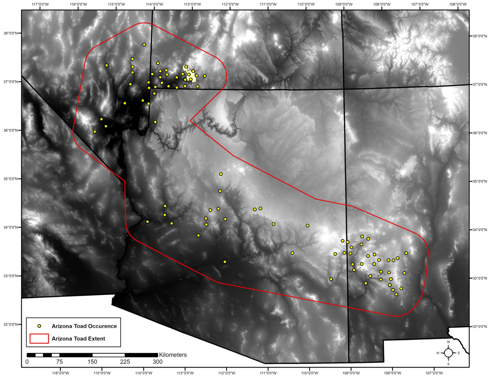
2.1. Study Area

Our study area included two scales of A. microscaphus distribution in North America. First, we studied A. microscaphus distribution on a localized landscape scale within Zion. Zion is located in the state of Utah in the western United States (Figure 1). Zion is located at the juncture of the Colorado Plateau, Mojave Desert, and Great Basin ecoregions. The elevation ranges from 2660 m at its highest point to 1117 m at its lowest point. Secondly, we studied A. microscaphus distribution on a range-wide scale across the full extent of its known and apparent range in North America. The ecoregions present at both scales included the Arizona–New Mexico Mountains, Great Basin, Mojave Desert, Colorado Plateau, and Utah High Plateaus ecoregions. The Arizona–New Mexico Mountains ecoregion is mostly semiarid with elevations ranging from 1371 to 3048 m and an average annual rainfall of 25–88 cm, which supports forests with perennial, intermittent, and ephemeral stream system microclimates. Vegetation below 1676 m consists of a surrounding desert habitat of juniper, yucca, stool, lechuguilla, prickly pear cactus, and mesquite. At elevations up to 2650 m, vegetation is dominated by semi-arid grasslands. The Mohave Desert ecoregion has a climate characterized by seasonal precipitation ranging from 8 to 25 cm and elevations consisting of majority desert plains and isolated mountains, ranging from −91 to 3344 m in elevation. The channel and stream characteristics consist mostly of seasonal runoff that filters through ephemeral drainage basins, with some of the runoff draining into the Colorado River [27]. The Colorado Plateau ecoregion has an elevation ranging from 1500 to 2100 m and has average annual temperatures ranging from 4° to 13 °C. The climate is arid to semi-arid, with an average annual precipitation of roughly 14 to 40 cm. The ecoregion is characterized by geographic features including broad plateaus, ancient volcanoes, and deep canyons [28]. In the Utah High Plateaus ecoregion, located to the far north of the study area, elevations range between 1500 to 4100 m. Precipitation is distributed throughout the year, ranging from 37.5 to 90 cm annually. An abundance of perennial streams drain into the Sevier, Virgin, and Colorado rivers [27].

2.2. Data Acquisition

2.2.1. Occurrence Data

Occurrence data for A. microscaphus were obtained using the Global Biodiversity Information Facility (GBIF; https://www.gbif.org/; accessed on 15 August 2020). To prepare the spatial data for the model, the occurrence points were downloaded and cleaned (i.e., the removal of duplicates and extreme outliers, and points located outside of the reasonable known range of the species). We filtered data to eliminate issues of spatial autocorrelation. Filtering was performed by removing localities that were within a 30 km radius of each other [29]. The spatial filtering step was performed using the SDMtoolbox with the tool ‘Spatially Rarefy Occurrence Data’. A distance of 30 km was chosen based upon the high spatial heterogeneity of the western mountains of the U.S. [30,31,32].

2.2.2. Spatial Scale and Resolution

The study area extent for the focal species was determined by constructing a convex hull fitted to the spatially filtered occurrence points, followed by a 50 km buffer around the hull. The convex hull was generated in ArcMap 10.6.1 using the ‘convex hull’ tool. This technique is used to reduce the overfitting of a model [29,33]. The hull was then used to clip the proceeding environmental variable rasters using the same extent, coordinate system, pixel count, and resolution. Each distribution (i.e., Zion-specific distribution and the complete distribution) was estimated based on data from their respective scales in order to improve the precision and accuracy of the models.
We used a 30 m grain size resolution for the environmental variable rasters. The grain size was determined primarily due to A. microscaphus being labeled as a habitat specialist and the need to delineate fine-scale habitat features (i.e., fragmentation, movement corridors) that may otherwise not be visible with a coarser grain resolution. The geomorphologic and remotely sensed covariates had a predetermined spatial resolution of a 30 m grain size and did not need further modifications to meet the grain size requirements. The climate data incorporated a two-step interpolation procedure based on the approach of Hutchinson and Xu [34] using weather station data (https://www.worldclim.org/data/worldclim21.html; accessed on 15 August 2020). A multiple linear regression model using Worldclim bioclimatic rasters and raster covariates followed by the thin plate spline (TPS) interpolation of the regression residuals was constructed in R [35] to create 30 m resolution climate rasters for the study extent of A. microscaphus [27,36,37]. Following the methodology of Hutchinson and Xu [34], using the ANUSPLIN climate interpolation package, the R package, MACHISPLIN, was used as an alternate method for climate data interpolation. This resulted in all model covariates having a 30 m resolution and allowed the models to run with finer-scale resolutions.

2.2.3. Elevation and Remote Sensing Data

Digital elevation model (DEM) rasters were obtained from the NASA Earthdata website (https://earthdata.nasa.gov/; accessed on 15 August 2020) and mosaicked together using ESRI ArcMap 10.6.1 to form a master DEM of the study area.
Data acquisition for the remotely sensed environmental variables was performed using the USGS website (https://earthexplorer.usgs.gov/; accessed on 15 August 2020) and included atmospherically corrected level-two Landsat satellite imagery. The scenes collected used atmospherically corrected level-two Landsat satellite imagery and dated back to a time frame that correlated with the average rainfall and temperature, coinciding positively during the breeding seasons for A. microscaphus. By using imagery from an average rainfall and temperature year, the potential effects of substantial land cover change were minimized. The imagery for A. microscaphus was obtained using Landsat 7 imagery with <5% cloud cover with various dates from May 2002. The remote sensing covariates included the normalized difference vegetation index (NDVI), for characterizing various aspects of land cover, and the bare soil index (BSI), for characterizing areas of bare soil.

2.2.4. Climatic Data

Climate data were downloaded from the WorldClim website (https://www.worldclim.org/data/index.html; accessed on 15 August 2020) and included 30 s of latitude and longitude (bio 30 s) raster datasets. The 19 variables represent annual trends and include the following: annual mean temperature (BIO1), mean diurnal range (BIO2), isothermality (BIO3), temperature seasonality (BIO4), max temperature of warmest month (BIO5), min temperature of coldest month (BIO6), temperature annual range (BIO7), mean temperature of wettest quarter (BIO8), mean temperature of driest quarter (BIO9), mean temperature of warmest quarter (BIO10), mean temperature of coldest quarter (BIO11), annual precipitation (BIO12), precipitation of wettest month (BIO13), precipitation of driest month (BIO14), precipitation seasonality (BIO15), precipitation of wettest quarter (BIO16), precipitation of driest quarter (BIO17), precipitation of warmest quarter (BIO18), and precipitation of coldest quarter (BIO19).

2.2.5. Environmental Variables

Other variables prepared for the modeling procedure were created using ArcMap 10.6.1. A slope raster was constructed using DEMs by calculating the maximum rate of change from the target cell and the eight surrounding neighbors in the raster. An aspect raster was also constructed using the DEM as the input data. We calculated a terrain ruggedness index (TRI) using the Vector Ruggedness Measure tool developed by Sappington et al. [38]. The topographic position index (TPI) was calculated using the difference between a cell elevation value and the average elevation of the surrounding neighborhood of the cell. TPI variables were created using the Land Facet Corridor Analysis version 1.2.605 toolbox [39]. The normalized difference vegetation index was calculated by obtaining relevant temporal Landsat imagery using the near-infrared and red color bands to generate an image displaying greenness. Lastly, the bare soil index (BSI) was created using the Raster Calculator tool [40].

2.3. Modeling Procedure

We modeled the potential distribution of A. microscaphus using a maximum entropy modeling approach (MaxEnt; [41]). We chose maximum entropy modeling over other available methods because it consistently results in better presence-only models [42,43]. The use of variables in the constructed models using the a priori process was followed by the removal of highly correlated variables using Pearson’s correlation coefficient. To adjust for multicollinearity, covariates displaying a high correlation above 0.9 were excluded in when preparing to build the model. We ran a total of 5 iterations for each model.

2.4. Environmental Variable Justification

2.4.1. Digital Elevation Model

Elevation is an important variable in habitat selection in that A. microscaphus elevation rarely exceeds 2700 m [44]. Elevation models were obtained from NASA’s Earthdata website and clipped to the study area.

2.4.2. Slope

The slope and steepness of a region significantly influence runoff, especially in mountainous areas like Zion. A. microscaphus is commonly found in areas with little to no slope, although this species prefers breeding and egg deposition in lightly flowing water [44].

2.4.3. Aspect

Aspect was chosen as a variable display solar radiation for A. microscaphus because it prefers to live in valley bottoms or areas with high canyon walls surrounding streams and rivers [44,45]. We hypothesize that this is important because this habitat could be influenced by solar exposure and a more southern-facing valley could constitute a preferred habitat.

2.4.4. Terrain Ruggedness Index

Because A. microscaphus prefers areas of relatively smoother topography, the terrain ruggedness index (TRI) should display a negative linear correlation within the MaxEnt models.

2.4.5. Topographic Position Index

The topographic position index was chosen for A. microscaphus to represent valley bottoms, which typically represent a high probability of habitat suitability due to the likelihood of alluvial accumulation and the presence of streams [44,45].

2.4.6. Normalized Difference Vegetation Index

Encroaching vegetation along the riparian habitat can potentially lead to the loss of a suitable habitat for A. microscaphus. We chose to utilize the NDVI because it quantifies vegetation along riparian areas that would negatively correlate with a suitable habitat choice for A. microscaphus.

2.4.7. Bare Soil Index

The bare soil index (BSI; [40]) was selected because A. microscaphus commonly occurs near areas displaying sandy soils or rocky slopes and sparse vegetation. The BSI relies on the short-wave infrared and red spectral bands to quantify soil mineral composition, while the blue and near-infrared bands display vegetative density.

2.5. Model Evaluation

2.5.1. Forecasting

Future model predictions were constructed using the bioclimatic variables from WorldClim (http://www.worldclim.org; accessed on 15 August 2020) for the years of 2050 and 2070. Yearly averages for 2050 were derived from the years (2041–2060), while 2070 projections were derived and averaged from (2061–2080). The Community Climate System Model (CCSM4) was used for forecasting. The spatial resolution for the future climate data was 30 s (~1 km2). Best and worst-case future climate scenarios were used for 2050 and 2070, with representative concentration pathways (RCPs) of 2.6 for the best-case scenario and 8.5 for the worst-case scenario. MaxEnt was used to compare the differences between the current suitable habitat in comparison to the best and worst-case future scenarios. Forecasting within MaxEnt used the same variables the current model uses, excluding the NDVI and BSI. The NDVI and BSI were removed because of inaccuracies in the projected future measurements of vegetation in bare soil.

2.5.2. Model Assessment and Validation

The MaxEnt outputs for A. microscaphus were calculated statistically by using the area under the receiver operating characteristic curve (AUC) to quantify the strength of the model, as the AUC is one of the most common statistics used to characterize model performance [46]. The AUC represents how well a model performs in predicting occurrences as opposed to a random selection of points. Model accuracy is considered excellent if the AUC is between 0.9 and 1, good if between 0.8 and 0.9, fair if between 0.7 and 0.8, poor if between 0.6 and 0.7, and failed if the AUC is between 0.5 and 0.6 [47].
The concept of the permutation importance of variables was used to assess the influence of predictor variables by measuring the drop in performance after randomly shuffling each variable’s values. The use of this technique in SDMs helps to prioritize key environmental drivers, ensuring more informed conservation decisions and resource allocations.
Additionally, we used the bootstrap method and a random selection of 25% of the occurrence points as test data to cross-validate all models. Cross-validation is preferred with smaller sample sizes to avoid repeating the same selection of occurrence points for later iterations.

3. Results

Of the 327 occurrence points for A. microscaphus, 87 rarified occurrence localities were left for analysis and 17 (25%) were used for test data (Figure 2). The AUC for the A. microscaphus model was 0.853 for the training data and 0.810 for the test data. The variables selected for inclusion in the models included the annual mean temperature, mean diurnal range, isothermality, precipitation seasonality, precipitation of coldest quarter, aspect, bare soil index, elevation, normalized difference vegetation index, ruggedness, slope, and topographic position index.

3.1. Model Performance

The top five permutation importance variables for A. microscaphus were as follows: annual mean temperature (22.9%), elevation (22.7%), isothermality (11.5%), NDVI (11.1%), and mean diurnal range (11.0%) (Table 1). Response curves (Figure 3) display the range of suitable conditions for each environmental variable independent of all other variables. The AUC for A. microscaphus was recorded as 0.9 for the training data and 0.8 for the test data, indicating good model accuracy.

3.2. Future Climate Trends

The current suitable habitat (>60% suitability) for A. microscaphus within Zion consists of 99,370 km2, which is 42.63% of the 233,078 km2 (Figure 4). When interpolated into the future across the entire range of the species, the 2050 RCP of 2.6 W/m2 habitat suitability decreased to 15,125 km2 or 6.48% (Figure 5). Further, the RCP of 8.5 W/m2 for the year 2050 increased to 7.59% suitability, with a surface area of 17,702 (km2), an increase from the previous RCP of 17.04% (Figure 5). The 2070 RCP of 2.6 W/m2 displayed an area of 17,942 km2, representing 7.7% suitability for the full range of A. microscaphus in North America (Figure 6). The suitable habitat area decreased considerably for the 2070 RCP of 8.5 W/m2 down to an area of 11,976 km2, representing a suitable area of 5.14% and a 33.25% decrease from the 2070 RCP of 2.6 W/m2 (Figure 6).

4. Discussion

Our models demonstrate the utility of remote sensing techniques in elucidating ecological relationships and improving our understanding of species ecology at the landscape scale. For example, the use of SDMs for the mapping of suitable habitats is a robust tool for spatially modeling species ecology in relation to geomorphological, remotely sensed, and climatic data to better understand landscape patterns that can then be used to frame management strategies or monitoring programs. Prior studies have undertaken habitat suitability analyses and the development of SDMs, demonstrating various methodologies and results [48,49]. However, these tools have not been widely applied to A. microscaphus, especially in the context of climate change. Therefore, our results aid in understanding this species’ habitat requirements at the landscape scale using remotely sensed data and a SDM framework, and how these may change under future global change scenarios. For example, our MaxEnt models generated a comprehensive map of the potential distribution of A. microscaphus, including Zion National Park, and reveal the unique contribution of the environmental variables to the prediction of habitat suitability both now and into the future.
Our results predict a substantial range-wide reduction in habitat suitability across climate scenarios from 2020 to 2050 and from 2050 to 2070, which has significant conservation implications for A. microscaphus due to its current at-risk status. Our results are significant and help to fill a much-needed gap in the understanding of A. microscaphus population declines. Recent declines have been primarily attributed to factors other than habitat and climate, such as the introduction of invasive species and hybridization with closely related bufonid toads [44]. Although these factors most definitely have had a significant impact on A. microscaphus populations and contemporary distributions, our results highlight the importance of habitat and climatic characteristics in shaping contemporary and future distributions of this species. Our results coincide with those of Suzart de Albuquerque et al. [45], which described the climatic factors (e.g., climate, topography, solar radiation) that significantly shape current and future (2081–2100) distributions of A. microscaphus. In their study, they also concluded that climate change may reduce habitat suitability and the distribution of A. microscaphus. Our model of the contemporary distribution of A. microscaphus includes not only the climatic and topographic variables proposed by Suzart de Albuquerque et al. [42], which were hypothesized to be the main drivers of the distribution of this species, but also includes the DEM (an absolute elevation value) and the NDVI (habitat vigor and health). The inclusion of the DEM and the NDVI improves the comprehensiveness of the representation of the absolute elevation and vegetation conditions, enhancing the predictive accuracy and ecological relevance of the model overall. Additionally, our forecasting models (i.e., predicted distributions in 2050, 2070) fill a temporal gap in predictions of distribution between now and 2100. The coupling of these models provides a time series of predictions of distributional changes in A. microscaphus over the next 80 years.
Zion is rich with microclimates that are affected by sharp landscape changes, including steep canyons, narrow and wide valleys, and steep slopes with differing aspects, which in addition to climatic variables, appear to influence the current and future distributions of A. microscaphus. Broadly, the identified geographic and climatic variables affect this microhabitat in ways that result in the increased or decreased identification of suitable habitats using fine-scale resolution models. Temperature contributed the most to model projections, with habitat suitability generally decreasing with an increase in the annual mean temperature above 10 °C. Because A. microscaphus is an ectotherm and relies heavily on the environment for thermoregulation, it is not surprising that temperature was influential in shaping this species’ distribution. Additionally, precipitation (i.e., precipitation seasonality, precipitation of coldest quarter), vegetation (e.g., the normalized difference vegetation index), and topography-related variables also contributed greatly to the models. Variables related to precipitation are also not surprisingly important to A. microscaphus distribution because water and moisture are often the primary limiting factors for amphibians, especially in arid environments such as southwestern North America. Amphibians are commonly known to rely heavily on moisture and temperature for proper physiological function. Additionally, vegetation and topography are likely important because of their effects on the available heat and moisture, which this species requires for continued persistence. However, vegetation likely plays a prominent role with regard to providing proper thermal and escape cover. It is likely that these variables represent important ecological aspects that affect natural and life history characteristics, which in turn influence species distribution. For example, the smaller-scale model (i.e., only within Zion) demonstrates that the most suitable habitat for A. microscaphus occurs along sloped rivers and streams and in valleys that typically host sandy soils, which appear to be essential for this species’ survival and persistence. This is further supported by the positive relationship between habitat suitability and the NDVI and its negative relationship with the Topographic Position Index (TPI). Specifically, a higher NDVI value indicates more green vegetation, which is indicative of higher water availability, more cover, and more preferable microclimates, which are characteristic of riparian habitats in this region. Additionally, a negative relationship with the TPI is indicative of the preference of A. microscaphus for valleys or lower-lying riparian areas. These are reasonable results considering that A. microscaphus is known to be strongly associated with riparian habitats throughout its range in the southwestern United States and that many of the individual variable relationships highlight important habitat characteristics that are common in this habitat type. Past studies have revealed similar ecological relationships. For example, Montgomery [44] found that broadscale habitat variables such as bioclimatic variables, the annual temperature range (lower probability with higher extreme temperatures), and precipitation (lower probability with decreasing rainfall) contributed to the probability of a habitat being occupied by A. microscaphus. Additionally, Montgomery [44] found that fine-scale variables such as shallow water, less woody debris, pebble substrate, and canopy cover contributed positively to A. microscaphus presence. This demonstrates the importance of riparian habitat conservation, which, based on our results, would likely benefit A. microscaphus populations greatly. As a result of these models and associated maps, land managers can visualize the probability of a suitable habitat for A. microscaphus and strategically allocate resources or construction projects in ways that benefit this species with more precise and accurate approaches. Moreover, the development of precise and accurate survey protocols, particularly those based on remotely sensed data, are especially important for A. microscaphus because of its status as an at-risk species and the limited knowledge of its habitat use at localized and landscape scales [50].
Based on the current climate projections, the A. microscaphus habitat will likely become increasingly more constrained across its range. For example, A. microscaphus habitat suitability decreased significantly as the models were projected further into the future with worst-case RCPs. A noticeable shift in habitat towards major river systems and away from smaller river systems can be observed in the 2070 forecasting maps, a concerning trend for this species considering its apparent association with riparian and riverine habitats. This may indicate a change in the amount of suitable riparian habitat available in the future as the climate warms and drought conditions increase in prevalence and duration. For instance, if smaller, more ephemeral streams in the landscape decrease as a result of rising temperatures and more severe and prolonged drought conditions, it is reasonable to expect populations of A. microscaphus to rely more heavily upon and persist near larger permanent river systems. This highlights a conservation and management target that can aid in bolstering or maintaining A. microscaphus populations in the North American landscape as conditions change. For example, we recommend that future management strategies should not only maintain larger, more persistent riparian habitats, but should also focus efforts on conserving smaller, more ephemeral habitats to increase their resilience during changing climatic conditions. This demonstrates the effectiveness of SDMs in deepening the understanding of species distributions across large spatial scales by elucidating the drivers that influence contemporary and future distributions, providing much-needed, and previously unattainable, information for the refinement of decision-making and management to combat the landscape-level effects of climate change.
Additionally, our models of the potential distribution of A. microscaphus can assist biologists and scientists in not only monitoring known populations, but also discovering populations by focusing surveys on areas of increased habitat suitability [2,3,4,51]. For species of concern, such as A. microscaphus, priority conservation areas can be easily and cost-effectively identified by MaxEnt models [2,3,4,52,53,54]. These models can also be used to guide population survey efforts for this species within Zion and across its range in the southwestern United States. For example, it has been found that as much as 70% of the time required to plan surveys for new species occurrences is saved when using SDMs to guide survey efforts [55]. This is an important consideration when aiming to maximize the utility of conservation resources that may need to conduct surveys on and monitor multiple species [51].
Due to many complex ecological processes, areas predicted to be suitable may not be inhabited by A. microscaphus; therefore, our models are better described as representations of the species’ fundamental, rather than realized, niche. Similar to many other distribution modeling studies, the ecological niche-based distribution models do have associated uncertainties and recognized weaknesses; therefore, our maps should only be used as estimations of the potential species distribution rather than definitive representations of the true distribution of this species [47]. A major limiting factor to conservation and management activities is often a lack of information about the spatial distribution of target species and how this may change over time [2,3,4,50]. As such, even theoretical habitat suitability and distribution models are highly useful for applied conservation, as they can outline distributions to a degree of certainty while also improving our understanding of the factors that shape species distributions, which allows for more thoughtful ecological insights [50].
Our results indicate that the current distribution of A. microscaphus in Zion National Park is a result of several different ecological and geological factors, but is also at risk of significant reduction across its range if current climate trends continue into the future. The future analysis and ground truthing of A. microscaphus distribution via field surveys is necessary to expand the model extent to the conterminous United States for a larger-scale analysis of the effects of climate and habitat change on suitable habitat. Also, expanding studies on local scales will help land managers and conservationists better understand how global and regional climate patterns influence local species populations for future needs. A noticeable lack of public literature regarding conservation efforts coupled with species models exemplifies the need to utilize SDMs based on their explicit conservation purposes. A standard protocol could objectively be assigned to private and government agencies to explore a middle ground to meet a standardized SDM approach for species on protected and private land alike.

Author Contributions

Conceptualization, S.M.D., D.L.K., C.M.S. and D.R.U.; Methodology, S.M.D., C.B.E., D.L.K., C.M.S., I.-K.H. and D.R.U.; Software, S.M.D., C.B.E., D.L.K., C.M.S., I.-K.H. and D.R.U.; Validation, S.M.D., D.L.K., I.-K.H. and D.R.U.; Formal Analysis, S.M.D., C.B.E., D.L.K., C.M.S., I.-K.H. and D.R.U.; Investigation, S.M.D., C.B.E., D.L.K., C.M.S., I.-K.H. and D.R.U.; Resources, S.M.D., D.L.K., C.M.S., I.-K.H. and D.R.U.; Data Curation, S.M.D., C.B.E., D.L.K., C.M.S., I.-K.H. and D.R.U.; Writing—Original Draft Preparation, S.M.D., C.B.E., D.L.K., C.M.S., I.-K.H. and D.R.U.; Writing—Review and Editing, S.M.D., C.B.E., D.L.K., C.M.S., I.-K.H. and D.R.U.; Visualization, S.M.D., C.B.E., D.L.K., C.M.S., I.-K.H. and D.R.U.; Supervision, S.M.D., C.B.E., D.L.K., C.M.S., I.-K.H. and D.R.U.; Project Administration, S.M.D., C.B.E., D.L.K., C.M.S., I.-K.H. and D.R.U.; Funding Acquisition, D.L.K., C.M.S., I.-K.H. and D.R.U. All authors have read and agreed to the published version of the manuscript.

Funding

This research was supported by a McIntire Stennis grant administered by the Arthur Temple College of Forestry and Agriculture at Stephen F. Austin State University.

Institutional Review Board Statement

Not applicable.

Informed Consent Statement

Not applicable.

Data Availability Statement

Publicly available datasets were analyzed in this study. This data can be found here: https://www.gbif.org/, (accessed on 15 August 2020).

Acknowledgments

This paper was written and prepared in part by U.S. Government employees on official time, and therefore it is in the public domain and not subject to copyright. This research was supported in part by the USDA Forest Service. The findings and conclusions in this publication are those of the author(s) and should not be construed to represent an official USDA, Forest Service, or U.S. Government determination or policy. This research was supported by a McIntire Stennis grant administered by the Arthur Temple College of Forestry and Agriculture at Stephen F. Austin State University.

Conflicts of Interest

The authors declare no conflict of interest.

References

  1. Raes, N. Partial versus Full Species Distribution Models. Nat. Conserv. 2012, 10, 127–138. [Google Scholar] [CrossRef]
  2. Addison, P.F.E.; Rumpff, L.; Bau, S.S.; Carey, J.M.; Chee, Y.E.; Jarrad, F.C.; McBride, M.F.; Burgman, M.A. Practical Solutions for Making Models Indespensible in Conservation Decision Making. Divers. Distrib. 2013, 19, 490–502. [Google Scholar] [CrossRef]
  3. Silva Angellieri, C.C.; Adams-Hosking, C.; de Barros Ferraz, K.M.P.M.; de Souza, M.P.; McAlpine, C.A. Using Species Distribution Models to Predict Potential Landscape Restoration Effects on Puma Conservation. PLoS ONE 2016, 11, e0145232. [Google Scholar] [CrossRef]
  4. Villero, D.; Pla, M.; Camps, D.; Ruiz-Olmo, J.; Brotons, L. Integrating species distribution modelling into decision-making to inform conservation actions. Biodivers. Conserv. 2016, 26, 251–271. [Google Scholar] [CrossRef]
  5. Melo-Merino, S.M.; Reyes-Bonilla, H.; Lira-Noriega, A. Ecological niche models and species distribution models in marine environments: A literature review and spatial analysis of evidence. Ecol. Model. 2020, 415, 108837. [Google Scholar] [CrossRef]
  6. Pourhallaji, M.; Dargahi, M.D.; Kami, H.G.; Hakimiabed, M. Species distribution modeling and environmental suitability of the Southern crested newt, Triturus karelinii (Strauch, 1870) (Amphibia: Caudata) in Iran. J. Wildl. Biodivers. 2021, 5, 44–52. [Google Scholar]
  7. Fong, G.A.; Dávila, N.V.; López-Iborra, G.M. Amphibian Hotspots and Conservation Priorities in Eastern Cuba Identified by Species Distribution Modeling. Biotropica 2015, 47, 119–127. [Google Scholar] [CrossRef]
  8. Pineda, E.; Lobo, J.M. Assessing the accuracy of species distribution models to predict amphibian species richness patterns. J. Anim. Ecol. 2009, 78, 182–190. [Google Scholar] [CrossRef]
  9. Spiers, J.A.; Oatham, M.P.; Rostant, L.V.; Farrell, A.D. Applying species distribution modelling to improving conservation based decisions: A gap analysis of Trinidad and Tobago’s endemic vascular plants. Biodivers. Conserv. 2018, 27, 2931–2949. [Google Scholar] [CrossRef]
  10. Gerick, A.A.; Munshaw, R.G.; Palen, W.J.; Combes, S.A.; O’Regan, S.M. Thermal physiology and species distribution models reveal climate vulnerability of temperate amphibians. J. Biogeogr. 2014, 41, 713–723. [Google Scholar] [CrossRef]
  11. Rawien, J.; Jairam-Doerga, S. Predicted Batrachochytrium dendrobatidis infection sites in Guyana, Suriname, and French Guiana using the species distribution model maxent. PLoS ONE 2022, 17, e0270134. [Google Scholar] [CrossRef] [PubMed]
  12. Trainor, A.M.; Schmitz, O.J.; Ivan, J.S.; Shenk, T.M. Enhancing species distribution modeling by characterizing predator–prey interactions. Ecol. Appl. 2014, 24, 204–216. [Google Scholar] [CrossRef] [PubMed]
  13. Battini, N.; Farías, N.; Giachetti, C.; Schwindt, E.; Bortolus, A. Staying ahead of invaders: Using species distribution modeling to predict alien species’ potential niche shifts. Mar. Ecol. Prog. Ser. 2019, 612, 127–140. [Google Scholar] [CrossRef]
  14. Peñalver-Alcázar, M.; Jiménez-Valverde, A.; Aragón, P. Niche differentiation between deeply divergent phylogenetic lineages of an endemic newt: Implications for Species Distribution Models. Zoology 2021, 144, 125852. [Google Scholar] [CrossRef] [PubMed]
  15. Rathore, M.K.; Sharma, L.K. Efficacy of species distribution models (SDMs) for ecological realms to ascertain biological conservation and practices. Biodivers. Conserv. 2023, 32, 3053–3087. [Google Scholar] [CrossRef]
  16. Laxton, M.R.; De Rivera, O.R.; Soriano-Redondo, A.; Illian, J.B. Balancing structural complexity with ecological insight in Spatio-temporal species distribution models. Methods Ecol. Evol. 2023, 14, 162–172. [Google Scholar] [CrossRef]
  17. Hernandez, P.A.; Graham, C.H.; Master, L.L.; Albert, D.L. The effect of sample size and species characteristics on performance of different species distribution modeling methods. Ecography 2006, 29, 773–785. [Google Scholar] [CrossRef]
  18. Ricketts, T.H. The Matrix Matters: Effective Isolation in Fragmented Landscapes. Am. Nat. 2001, 158, 87–99. [Google Scholar] [CrossRef]
  19. Vrba, E.S. Ecology in relation to speciation rates: Some case histories of Miocene-Recent mammal clades. Evol. Ecol. 1987, 1, 283–300. [Google Scholar] [CrossRef]
  20. Dodd, C.K. Frogs of the United States and Canada; John Hopkins University Press: Baltimore, MD, USA, 2013; pp. 127–132. [Google Scholar]
  21. Blais, B.; Ryan, M.J.; Gustafson, G.; Giermakowski, J.T. Natural History Notes. Herpetol. Rev. 2016, 47, 436–438. [Google Scholar]
  22. Sullivan, B.K.; Lamb, T. Hybridization Between the Toads Bufo microscaphus and Bufo woodhousii in Arizona: Variation in Release Calls and Allozymes. Herpetologica 1988, 44, 325–333. [Google Scholar]
  23. Ryan, M.J.; Latella, I.M.; Giermakowski, J.T.; Snell, H.L. Final Report: Status of the Arizona Toad (Anaxyrus microscaphus) in New Mexico; New Mexico Department of Game and Fish: Santa Fe, NM, USA, 2015; 35p.
  24. Sweet, S.S. Initial Report on the Ecology and Status of the Arroyo Toad (Anaxyrus Microscaphus Californicus) on the Los Padres National Forest of Southern California, with Management Recommendations; Contract Report to USDA; Forest Service, Los Padres National Forest: Goleta, CA, USA, 1992; p. 198.
  25. Schwaner, T.D.; Sullivan, B.K. Fifty Years of Hybridization: Introgression Between the Arizona Toad (Bufo microscaphus) and Woodhouse’s Toad (B. woodhousii) Along Beaver Dam Wash in Utah. Herpetol. Conserv. Biol. 2009, 4, 198–206. [Google Scholar]
  26. Hammerson, G.; Schwaner, T.D. Anaxyrus microscaphus. In IUCN 2011 IUCN Red List of Threatened Species; Version 2011.2; IUCN: Gland, Switzerland, 2004. [Google Scholar]
  27. McNab, W.H.; Avers, P.E. Ecological Subregions of the United States; Section Descriptions; USDA Forest Service, Ecosystem Management: Washington, DC, USA, 1994; Volume 5.
  28. Sleeter, B.M.; Sohl, T.L.; Bouchard, M.A.; Reker, R.R.; Soulard, C.E.; Acevedo, W.; Griffith, G.E.; Sleeter, R.R.; Auch, R.F.; Sayler, K.L.; et al. Scenarios of land use and land cover change in the conterminous United States: Utilizing the special report on emission scenarios at ecoregional scales. Glob. Environ. Change 2012, 22, 896–914. [Google Scholar] [CrossRef]
  29. Brown, J.L. SDMtoolbox: A Python-based GIS Toolkit for Landscape Genetic, Biogeographic, and Species Distribution Model Analyses. Methods Ecol. Evol. 2014, 5, 694–700. [Google Scholar] [CrossRef]
  30. Pearson, R.G.; Raxworthy, C.J.; Nakamura, M.; Peterson, A.T. Predicting species distributions from small numbers of occurrence records: A test case using cryptic geckos in Madagascar. J. Biogeogr. 2006, 34, 102–117. [Google Scholar] [CrossRef]
  31. Anderson, R.P.; Raza, A. The effect of the extent of the study region on GIS models of species geographic distributions and estimates of niche evolution: Preliminary tests with montane rodents (genus Nephelomys) in Venezuela. J. Biogeogr. 2010, 37, 1378–1393. [Google Scholar] [CrossRef]
  32. Boria, R.A.; Olson, L.E.; Goodman, S.M.; Anderson, R.P. Spatial filtering to reduce sampling bias can improve the performance of ecological niche models. Ecol. Model. 2014, 275, 73–77. [Google Scholar] [CrossRef]
  33. Williams, J.N.; Seo, C.; Thorne, J.; Nelson, J.K.; Erwin, S.; O’Brien, J.M.; Schwartz, M.W. Using Species Distribution Models to Predict New Occurrences for Rare Plants. Divers. Distrib. 2009, 15, 565–576. [Google Scholar] [CrossRef]
  34. Hutchinson, M.F.; Xu, T. ANUSPLIN Version 4.4 User Guide; Fenner School of Environment and Society, Australian National University: Canberra, ACT, Australia, 2013. [Google Scholar]
  35. R Core Team. R: A Language and Environment for Statistical Computing; R Foundation for Statistical Computing: Vienna, Austria, 2022; Available online: https://www.R-project.org/ (accessed on 15 August 2020).
  36. Morgan, B.; Guénard, B. New 30 m resolution Hong Kong climate, vegetation, and topography rasters indicate greater spatial variation than global grids within an urban mosaic. Earth Syst. Sci. Data 2019, 11, 1083–1098. [Google Scholar] [CrossRef]
  37. Meineri, E.; Hylander, K. Fine-grain, large-domain climate models based on climate station and comprehensive topographic information improve microrefugia detection. Ecography 2017, 40, 1003–1013. [Google Scholar] [CrossRef]
  38. Sappington, J.M.; Longshore, K.M.; Thompson, D.B. Quantifying Landscape Ruggedness for Animal Habitat Analysis: A Case Study Using Bighorn Sheep in the Mojave Desert. J. Wildl. Manag. 2007, 71, 1419–1426. [Google Scholar] [CrossRef]
  39. Jenness, J. Topographic Position Index Extension for ArcView 3.x. Jenness Enterprises. 2006. Available online: http://www.jennessent.com/arcview/tpi.htm (accessed on 15 August 2020).
  40. Zhao, H.M.; Chen, X. Use of Normalized Difference Bareness Index in Quickly Mapping Bare Areas from TM/ETM+. Geosci. Remote Sens. Symp. 2003, 3, 1666–1668. [Google Scholar]
  41. Phillips, S.J.; Dudík, M.; Schapire, R.E. Maxent Software for Modeling Species Niches and Distributions. Version 3.4.1. 2017. Available online: http://biodiversityinformatics.amnh.org/open_source/maxent/ (accessed on 15 August 2020).
  42. Esquivel, D.A.; Penagos, A.P.; García, R.S.; Bennett, D. New records of Pygmy Round-eared Bat, Lophostoma brasiliense Peters, 1867 (Chiroptera, Phyllostomidae), and updated distribution in Colombia. Check List 2020, 16, 277–285. [Google Scholar] [CrossRef]
  43. Stryszowska, K.M.; Johnson, G.; Mendoza, L.R.; Langen, T.A. Species Distribution Modeling of the Threatened Blanding’s Turtle’s (Emydoidea blandingii) Range Edge as a Tool for Conservation Planning. J. Herpetol. 2016, 50, 366–373. [Google Scholar] [CrossRef]
  44. Montgomery, B. Occupy ToadStreet: Occupancy and Habitat Use of the Arizona Toad in Streams of Arizona. Master’s Thesis, Arizona State University, Phoeniz, AZ, USA, 2023; 61p. [Google Scholar]
  45. De Albuquerque, F.S.; Bateman, H.L.; Ryan, M.J.; Montgomery, B. Model transferability and predicted response of a dryland anuran to climate change in the Southwest United States. J. Biogeogr. 2023, in press. [Google Scholar] [CrossRef]
  46. Yackulic, C.B.; Chandler, R.; Zipkin, E.F.; Royle, J.A.; Nichols, J.D.; Grant, E.H.C.; Veran, S. Presence-only Modelling Using MAXENT: When Can We Trust the Inferences? Methods Ecol. Evol. 2013, 4, 236–243. [Google Scholar] [CrossRef]
  47. Swets, J.A. Measuring the accuracy of diagnostic systems. Science 1998, 240, 1285–1293. [Google Scholar] [CrossRef] [PubMed]
  48. Ayoro, J.H.; Nicolas, V.; Segniagbeto, G.H.; Hema, E.M.; Ohler, A.; Kabré, G.B. Potential impact of climate change on spatial distribution of two savannah amphibian species in West Africa. Afr. J. Ecol. 2023, in press. [Google Scholar] [CrossRef]
  49. Zhang, Z.; Mammola, S.; Liang, Z.; Capinha, C.; Wei, Q.; Wu, Y.; Zhou, J.; Wang, C. Future climate change will severely reduce habitat suitability of the Critically Endangered Chinese giant salamander. Freshw. Biol. 2020, 65, 971–980. [Google Scholar] [CrossRef]
  50. Ryan, M.J.; Giermakowski, J.T.; Latella, I.M.; Snell, H.L. No evidence of hybridization between the Arizona toad (Anaxyrus microscaphus) and Woodhouse’s toad (A. woodhousii) in New Mexico, USA. Herpetol. Conserv. Biol. 2017, 12, 565–575. [Google Scholar]
  51. Thurtell, L.; Rajanathan, R.; Thomas, P.; Ballard, G.; Bayne, P.; Vernes, K. Predictively modeling the distribution of the threatened brush-tailed rock-wallaby (Petrogale penicillate) in Oxley Wild Rivers National Park, north-eastern New South Wales, Australia. Wildl. Res. 2022, 49, 169–182. [Google Scholar] [CrossRef]
  52. Liang, C.T.; Stohlgren, T.J. Habitat suitability of patch types: A case study of the Yosemite toad. Front. Earth Sci. 2011, 5, 217–228. [Google Scholar] [CrossRef]
  53. Giovannini, A.; Seglie, D.; Giacoma, C. Identifying priority areas for conservation of spadefoot toad, Pelobates fuscus insubricus using a maximum entropy approach. Biodivers. Conserv. 2014, 23, 1427–1439. [Google Scholar] [CrossRef]
  54. Ganesh, S.R.; Brihadeesh, S.; Narayana, B.L.; Hussain, S.; Kumar, G.C. A contribution on morphology and distribution of the Rock Toad, Duttaphrynus hololius (Günther, 1876) with first report on deformity, calling and breeding behaviours (Amphibia: Anura: Bufonidae). Asian J. Conserv. Biol. 2020, 9, 71–78. [Google Scholar]
  55. Guisan, A.; Brönnimann, O.; Engler, R.; Vust, M.; Yoccoz, N.G.; Lehmann, A.; Zimmermann, N.E. Using Niche-Based Models to Improve the Sampling of Rare Species. Conserv. Biol. 2006, 20, 501–511. [Google Scholar] [CrossRef]
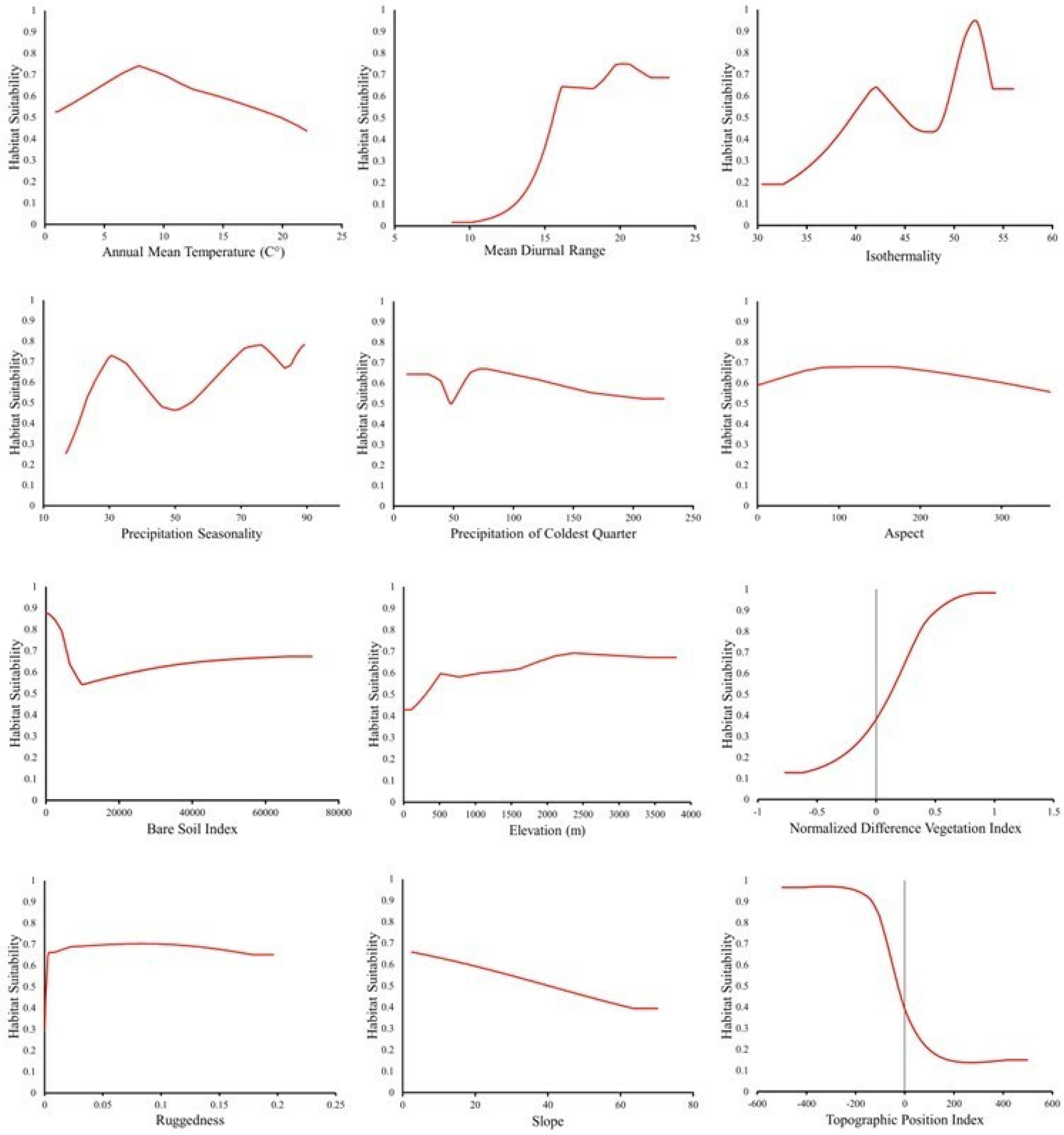
Figure 1. Location of Zion National Park in southwestern Utah, U.S.
Ecologies 04 00050 g001
Figure 2. The study extent and range of occurrence of localities for Anaxyrus microscaphus across the full extent of the known species range.
Ecologies 04 00050 g002
Figure 3. Partial dependence plots displaying the marginal response of the 12 environmental variables selected for Anaxyrus microscaphus in the MaxEnt model. Each response curve demonstrates the range of suitability for each environmental variable if each variable were used to create a MaxEnt model independent of the outside influence of other variables.
Ecologies 04 00050 g003
Figure 4. MaxEnt model output for 30 m resolution habitat suitability maps for Anaxyrus microscaphus in Zion National Park, Utah, USA. Suitability classes describe the ranking of habitat preference for the species being modeled. Models were created using MaxEnt. Subfigure indicates the location (red square) of the suitability map relative to the state of Utah, USA.
Ecologies 04 00050 g004
Figure 5. Forecasting SDM of Anaxyrus microscaphus contrasting the suitable habitat for future best and worst-case climate scenarios with the representative concentration pathways that describe greenhouse gas concentrations of 2.6 W/m2 and 8.5 W/m2 for the year 2050. Subfigure indicates the location (red square) of the suitability map relative to the state of Utah, USA.
Ecologies 04 00050 g005
Figure 6. Forecasting SDM of Anaxyrus microscaphus contrasting the suitable habitat for future best and worst-case climate scenarios with representative concentration pathways that describe greenhouse gas concentrations of 2.6 W/m2 and 8.5 W/m2 for the year 2070. Subfigure indicates the location (red square) of the suitability map relative to the state of Utah, USA.
Ecologies 04 00050 g006
Table 1. Permutation importance values for each bioclimatic variable within the MaxEnt model for the Arizona toad. The permutation value is determined by randomly permuting the values of each independent variables against the training points. Values are then normalized to provide percentages; higher values suggest a greater influence on the model.
VariablePermutation Importance (%)
Annual Mean Temperature22.9
Elevation22.7
Isothermality11.5
Normalized Difference Vegetation Index11.1
Mean Diurnal Range11.0
Precipitation Seasonality5.7
Topographic Position Index3.5
Slope3.2
Precipitation of Coldest Quarter2.7
Ruggedness2.4
Aspect2.1
Bare Soil Index1.2
Disclaimer/Publisher’s Note: The statements, opinions and data contained in all publications are solely those of the individual author(s) and contributor(s) and not of MDPI and/or the editor(s). MDPI and/or the editor(s) disclaim responsibility for any injury to people or property resulting from any ideas, methods, instructions or products referred to in the content.

