Evaluating the Effectiveness of Machine Learning for Alzheimer’s Disease Prediction Using Applied Explainability

Abstract

Early and accurate diagnosis of Alzheimer’s disease (AD) is critical for patient outcomes yet presents a significant clinical challenge. This study evaluates the effectiveness of four machine learning models—Logistic Regression, Random Forest, Support Vector Machine, and a Feed-Forward Neural Network—for the five-class classification of AD stages. We systematically compare model performance under two conditions, one including cognitive assessment data and one without, to quantify the diagnostic value of these functional tests. To ensure transparency, we use SHapley Additive exPlanations (SHAPs) to interpret the model predictions. Results show that the inclusion of cognitive data is paramount for accuracy. The RF model performed best, achieving an accuracy of 84.4% with cognitive data included. Without this, performance for all models dropped significantly. SHAP analysis revealed that in the presence of cognitive data, models primarily rely on functional scores like the Clinical Dementia Rating—Sum of Boxes. In their absence, models correctly identify key biological markers, including PET (positron emission tomography) imaging of amyloid burden (FBB, AV45) and hippocampal atrophy, as the next-best predictors. This work underscores the indispensable role of cognitive assessments in AD classification and demonstrates that explainable AI can validate model behavior against clinical knowledge, fostering trust in computational diagnostic tools.

1. Introduction

Alzheimer’s disease (AD) is an irreversible, progressive brain disorder that severely impairs memory and cognitive functions, leading to significant challenges in daily activities. It is a leading cause of dementia and was associated with 5.8 million cases in the United States in 2020 alone, a number projected to more than double by the mid-century [1]. Genetic research over recent decades has identified several genes correlated with AD causality, enriching our understanding of its biological underpinnings [2,3,4,5].

The trajectory of Alzheimer’s disease encompasses seven stages: preclinical, asymptomatic cerebral amyloidosis, subjective cognitive decline, mild cognitive impairment (MCI), mild AD, moderate AD, and severe AD [6]. Our study focuses on a five-class classification task distinguishing cognitively normal (CN) individuals, those with subjective memory concerns (SMC), early mild cognitive impairment (EMCI), late mild cognitive impairment (LMCI) and those with AD.

Conventional diagnostic methods including clinical evaluations, cognitive assessments, magnetic resonance imaging (MRI), and positron emission tomography (PET) scans offer high accuracy but involve significant cost and invasiveness [7]. While these imaging modalities remain critical biomarkers for amyloid and tau pathology, integrating non-invasive measures such as demographic, genetic, and questionnaire-based data may enhance early detection accessibility. Recent surveys of AI and explainable AI in clinical decision support, including applications to neurodegenerative disorders, have identified best practices, common pitfalls, and emerging directions for ML and DNN models in healthcare [8,9,10,11,12].

Previous Alzheimer’s disease prediction efforts using “black box” models such as extreme gradient boosting (XGBoost) and SVM have demonstrated strong classification performance but offered little insight into how inputs drive each prediction. For example, an XGBoost model achieved over 90% accuracy in early AD detection without any post hoc interpretation of feature contributions, and traditional SVM approaches similarly report high accuracy without transparent decision rationale [13,14]. SHAP overcomes these limitations by decomposing a model’s output into additive feature attributions, yielding both global importance rankings and patient-level explanations that clinicians can audit for trust and reliability [15]. Other research has also focused on early diagnosis by applying machine learning to various data modalities. For example, some studies have successfully used RF and Neural Networks (NNs) for early detection, employing methods like Gini importance to rank predictive variables [16]. While useful, Gini importance provides a global-level ranking and lacks the granular, instance-level insight that SHAP provides for auditing individual predictions.

We evaluated four predictive models: logistic regression (LR), random forest (RF), support vector machine (SVM), and feedforward neural network (FNN) on the ADNI merge dataset, which includes cognitive assessments, imaging biomarkers, genetic variants, and demographic measures (non-biological data points capturing contextual and functional information such as age, sex, education level, lifestyle factors, and self-reported cognitive scores). We then applied SHAP explainability techniques to each model to reveal both global feature importance and patient-level explanations, highlighting how cognitive assessments versus imaging features drive the predictions [17,18].

Early diagnosis is crucial for improving patient outcomes; by elucidating model behavior with XAI, we aim to foster clinician trust and pave the way for transparent, data-driven decision support in Alzheimer’s disease care. Launched in 2004, ADNI is a critical study aimed at identifying biomarkers for Alzheimer’s disease through clinical, genetic, and imaging data [19]. The ADNI merge dataset, a comprehensive amalgamation of ADNI1, ADNI-GO, and ADNI2 phases, includes detailed clinical outcomes, demographic data, genetic profiles, and critical biomarkers like amyloid and tau [20]. It is valuable for developing predictive models using advanced analytics such as machine learning and deep learning. This dataset comprises clinical, imaging, and genetic data and includes significant information collected through detailed cognitive assessments. These cognitive assessments cover various topics crucial for understanding the broader context of Alzheimer’s disease, including participants’ lifestyle factors, cognitive functions, and overall health status. While the inclusion of these cognitive assessments enriches the dataset, providing nuanced information about the progression and risk factors associated with Alzheimer’s disease, there is also a risk that they might lead to redundancy. This overlap could skew the predictions by weighing the models more heavily towards duplicated information from the datasets and the cognitive assessments.

By comparing models trained on the entire ADNI merge dataset to those trained exclusively on data subsets, excluding the cognitive assessments, this study aims to discern the value of these non-biological data points added. This comparison is essential for determining whether the cognitive assessments contribute meaningful insights that improve model performance or if they introduce noise and redundancy that could potentially skew the predictions. Additionally, the primary aim of this research is to compare the results between different predictive models, specifically machine learning models and deep neural networks, focusing on their explainability within the context of AD prediction. This multifaceted analysis will help optimize the dataset for future research and refine the models for higher accuracy and reliability in predicting Alzheimer’s disease progression and onset. Furthermore, by assessing the transparency and interpretability of these models, the study enhances understanding of how decisions are made, thus increasing trust and applicability in clinical settings. This approach underscores the importance of meticulously examining all data dimensions and their roles in enhancing the capabilities of predictive models in neurodegenerative diseases.

At baseline (n = 2399), the class distribution is imbalanced (Table 1), with LMCI the largest group (28.51%; n = 684) and SMC the smallest (14.46%; n = 347). It further includes demographic measures, clinical assessments, imaging biomarkers, genetic variants, and CSF markers (Table 2), offering a comprehensive set of predictors. The ‘Non-baseline duplicates’ column in Table 2 quantifies the number of variables (e.g., AV45) that exist in the raw dataset alongside a specific baseline-suffixed version (e.g., AV45_bl). As this study uses a strict baseline-only (cross-sectional) design, these 50 unsuffixed columns, which represent data from other time points, were removed during preprocessing to prevent temporal leakage. This ensured that only the baseline variables were used for analysis. To correct for the overrepresentation of cognitively normal cases and underrepresentation of Alzheimer’s disease cases, class weights inversely proportional to these baseline frequencies are applied during model training, ensuring that each diagnostic group contributes appropriately to the learning process.

Table 1. Cohort size and class distribution at baseline.

Diagnostic Group	N Subjects (n = 2399)	% of Cohort
Cognitively Normal (CN)	541	22.55%
Subjective Memory Concerns (SMC)	347	14.46%
Early Mild Cognitive Impairment (EMCI)	417	17.38%
Late Mild Cognitive Impairment (LMCI)	684	28.51%
Alzheimer’s Disease (AD)	410	17.09%

Table 2. Number of variables by category in the ADNI merge dataset.

Feature Type	Number of Variables	Non-Baseline Duplicates
Administrative metadata	9	0
Demographic measures	6	0
Genetic variants	1	0
Cognitive assessments	60	30
Imaging PET biomarkers	8	4
CSF biomarkers	6	3
Time variables	4	2
Target labels	2	1
Total	116	50

2. Materials and Methods

2.1. Data Source and Cohort

Analyses use the Alzheimer’s Disease Neuroimaging Initiative (ADNI) merged table (ADNIMERGE) under a cross-sectional, baseline-only design. Records are restricted to the baseline visit (VISCODE = “bl”), and predictors are limited to variables with the baseline suffix “_bl”. Where baseline-suffixed and unsuffixed versions co-exist, unsuffixed duplicates are removed to avoid temporal leakage. Administrative and time-keeping fields (e.g., RID, PTID, site/protocol, EXAMDATE, Month/M, Month_bl/Years_bl, FSVERSION, IMAGEUID_bl) are removed. The outcome is baseline clinical diagnosis (DX_bl) encoded as a five-class label: CN, SMC, EMCI, LMCI, AD. Two analysis tables are produced: a with-cognition table that retains cognitive tests and a no-cognition table created by removing them. After preprocessing, each table contains 2399 rows; the with-cognition table has 35 columns, and the no-cognition table has 21 columns.

2.2. Study Design and Partitioning

All statistical analyses and model development were conducted using Python (version 3.9.9; Python Software Foundation, Wilmington, DE, USA). To ensure methodological rigor and prevent data leakage, the complete, preprocessed dataset is first partitioned into a stratified 80/20 train/test split (1919 training rows, 480 test rows). This partition is performed prior to any feature imputation, scaling, or selection. All subsequent preprocessing steps are encapsulated in scikit-learn pipelines that are fitted only on the 80% training data. The resulting transformations are then applied, without refitting, to the 20% hold-out test set to generate a valid performance estimate. To address class imbalance in the classical models, class weights are set inversely proportional to class frequency (the “balanced” scheme), where

$${\mathit{w}}_{\mathit{c}}=\mathit{ }{\displaystyle \frac{\mathit{N}}{\mathit{K}\mathit{ }{\mathit{n}}_{\mathit{c}}}}=\mathit{ }{\displaystyle \frac{\mathbf{1}}{\mathit{K}\mathit{ }{\mathit{p}}_{\mathit{c}}}}\mathit{ }.$$

(1)

Here, ${\mathit{w}}_{\mathit{c}}$ is the computed weight for a given class $\mathit{c}$, $\mathit{N}$ is the total number of training samples, $\mathit{K}$ is the total number of classes (five in this study), ${\mathit{n}}_{\mathit{c}}$ is the number of samples belonging to class $\mathit{c}$, and ${\mathit{p}}_{\mathit{c}}$ is the prevalence of class $\mathit{c}$ in the training data. A fixed analysis seed of 42 is used for data splitting and model initialization to aid reproducibility.

2.3. Preprocessing Pipeline

A robust preprocessing workflow is defined using scikit-learn’s (version 1.5.2; Inria, Le Chesnay-Rocquencourt, France) Pipeline and ColumnTransformer objects. This approach ensures that all feature transformations are learned solely from the training partition. First, rows with more than 30% missing fields are removed. The remaining features are then separated into two distinct streams.

Numerical features are processed using a pipeline that first imputes missing values with a five-nearest-neighbor imputer (KNNImputer) and subsequently standardizes all features using StandardScaler (Z-score). Categorical features, which include demographic data (such as gender, marital status, education level, etc.), genetic status (APOE4), and certain CSF biomarkers (ABETA, TAU, PTAU), are processed with a separate pipeline. This categorical stream first imputes missing values with a constant “Missing” string (SimpleImputer) and then converts the features into a numerical format using OneHotEncoder, which is configured to ignore unknown categories encountered in the test data.

2.4. Feature Selection and Standardization

The ColumnTransformer (containing the numerical and categorical pipelines) is combined into a single Pipeline object with subsequent feature selection steps. Immediately following the preprocessing, a VarianceThreshold transformer is applied to remove any zero-variance features that may have been created during one-hot encoding. Following this, univariate ANOVA F-test screening (SelectKBest) is used to select the most informative features. The number of retained features (k) is tuned as a key hyperparameter during model training, with the search space set to 20, 50, or ‘all’ (all features remaining after the variance threshold). The F-statistics for a given feature ${\mathit{x}}_{\mathit{j}}$ is defined as:

$${\mathit{F}}_{\mathit{j}}=\mathit{ }{\displaystyle \frac{{\mathrm{SS}}_{\mathrm{between}}/\left(\mathit{K}-\mathbf{1}\right)}{{\mathrm{SS}}_{\mathrm{within}}/\left(\mathit{N}-\mathit{K}\right)}},\mathit{ }{\mathrm{SS}}_{\mathrm{between}}=\mathit{ }\sum _{\mathit{c}=\mathbf{1}}^{\mathit{K}}{\mathit{n}}_{\mathit{c}}{\left({\overline{\mathit{x}}}_{\mathit{j},\mathit{ }\mathit{c}}-\mathit{ }{\overline{\mathit{x}}}_{\mathit{j}}\right)}^{\mathbf{2}},\mathit{ }{\mathrm{SS}}_{\mathrm{within}}=\mathit{ }\sum _{\mathit{c}=\mathbf{1}}^{\mathit{K}}\left({\mathit{n}}_{\mathit{c}}-\mathit{ }\mathbf{1}\right){\mathit{s}}_{\mathit{j},\mathit{c}}^{\mathbf{2}}$$

(2)

Retained numeric predictors were z-scaled as described in preprocessing. This integrated pipeline ensures that feature selection is part of the cross-validation and training process, treating it as a component of the model itself to avoid data leakage.

2.5. Models and Training Procedures

Four model families are evaluated: multinomial LR, SVM, RF, and FNN. The placement of screening, scaling, nested cross-validation, and calibration is summarized in Figure 1.

Figure 1. Overall pipeline.

2.5.1. Logistic Regression (Multinomial, L2)

A multinomial, L2-regularized logistic regression fits after feature screening and z-scaling. The regularization strength C is tuned over four values (0.01, 0.1, 1, 10), and the maximum number of iterations is set to 1000. The selected C was chosen by an inner three-fold grid search within an outer five-fold scheme. For class $\mathit{k}$, the linear score is ${\mathit{z}}_{\mathit{k}}\left(\mathit{x}\right)={\mathit{\beta }}_{\mathit{k}}^{\mathit{\top }}\tilde{\mathit{x}}+{\mathit{b}}_{\mathit{k}}$ with standardized $\tilde{\mathit{x}}$, and the SoftMax likelihood is

$$\mathit{p}\left(\mathit{y}=\mathit{k}|\mathit{x}\right)=\mathit{ }{\displaystyle \frac{\exp \left({\mathit{z}}_{\mathit{k}}\right)}{\mathbf{\sum }_{\mathit{c}=\mathbf{1}}^{\mathit{K}}\exp \left({\mathit{z}}_{\mathit{k}}\right)}}.$$

(3)

Training minimizes the class-weighted multinomial cross-entropy with L2 penalty:

$$\underset{\left\{{\mathit{\beta }}_{\mathit{k}},\mathit{ }{\mathit{ b}}_{\mathit{k}}\right\}}{\mathbf{min}}-\sum _{\mathit{i}=\mathbf{1}}^{\mathit{N}}\sum _{\mathit{k}=\mathbf{1}}^{\mathit{K}}\mathbf{1}\left[{\mathit{y}}_{\mathit{i}}=\mathit{k}\right]{\mathbf{log}}_{\mathit{p}}\left(\mathit{y}=\mathit{k}|{\mathit{x}}_{\mathit{i}}\right){\mathit{w}}_{{\mathit{y}}_{\mathit{i}}}+\mathit{ }\mathit{\lambda }\sum _{\mathit{k}=\mathbf{1}}^{\mathit{K}}{‖{\mathit{\beta }}_{\mathit{k}}‖}_{\mathbf{2}}^{\mathbf{2}},\mathit{ }\mathit{ }\mathit{ }\mathit{ }\mathit{ }\mathit{ }\mathit{ }\mathit{ }\mathit{\lambda }=\mathit{ }\mathbf{1}/\mathit{c},$$

(4)

where $\mathit{i}$ indexes $\mathit{N}$ training samples, $\mathit{k}$ indexes $\mathit{K}$ classes, $\mathbf{1}(·)$ is the indicator function, ${\mathit{w}}_{{\mathit{y}}_{\mathit{i}}}$ is the weight for class ${\mathit{y}}_{\mathit{i}}$, ${\mathit{\beta }}_{\mathit{k}}$ and ${\mathit{b}}_{\mathit{k}}$ are the weights and bias for class $\mathit{k}$, and $\mathit{\lambda }$ is the L2 regulation strength.

This specification provides a calibrated linear reference model with directionally interpretable coefficients and improved numerical stability in the presence of correlated predictors.

2.5.2. Support Vector Machine (One-Vs-Rest; RBF Kernels)

After screening and z-scaling, SVMs are trained in a one-vs-rest fashion using a radial-basis-function (RBF) kernel. The regularization parameter $\mathit{C}$ is evaluated at three levels (0.1, 1, 10). The RBF with parameter $\mathit{\gamma }$ follows the library’s scale and auto options. For each binary subproblem, the linear soft-margin primal is

$$\underset{\mathit{w},\mathit{b},\mathit{\xi }}{\mathbf{min}}{\displaystyle \frac{\mathbf{1}}{\mathbf{2}}}{‖\mathit{w}‖\mathit{ }}_{\mathbf{2}}^{\mathbf{2}}+\mathit{C}\sum _{\mathit{i}=\mathbf{1}}^{\mathit{N}}{\mathit{\xi }}_{\mathit{i}}\mathit{ }\mathit{ }\mathit{ }\mathit{ }\mathit{ }\mathit{ }\mathrm{s}.\mathrm{t}.\mathit{ }\mathit{ }\mathit{ }\mathit{ }\mathit{ }\mathit{ }{\mathit{y}}_{\mathit{i}}({\mathit{w}}^{\mathit{\top }}{\tilde{\mathit{x}}}_{\mathit{i}}+\mathrm{b})\ge \mathbf{1}-{\mathit{\xi }}_{\mathit{i}}\mathit{ },{\mathit{\xi }}_{\mathit{i}}\ge 0,$$

(5)

and the kernel decision function is

$$\mathit{f}\left(\mathit{x}\right)=\mathit{ }\sum _{\mathit{i}=\mathit{ }\mathbf{1}}^{\mathit{N}}{\mathit{\alpha }}_{\mathit{i}}{\mathit{y}}_{\mathit{i}}\mathit{K}\left({\tilde{\mathit{x}}}_{\mathit{i}},\tilde{\mathit{x}}\right)+\mathit{b},\mathit{ }\mathit{ }\mathit{ }\mathit{ }{\mathit{K}}_{\mathrm{RBF}}\left(\mathit{x},\mathit{ }{\mathit{x}}^{\mathbf{\prime }}\right)=\mathit{ }\exp \left(-\mathit{\gamma }{‖\mathit{x}-{\mathit{x}}^{\mathbf{\prime }}‖}_{\mathbf{2}}^{\mathbf{2}}\right),$$

(6)

where $\mathit{w}$ and $\mathit{b}$ define the hyperplane, ${\mathit{\xi }}_{\mathit{i}}$ are slack variables, $\mathit{C}$ is the regularization parameter, ${\mathit{\alpha }}_{\mathit{i}}$ are the learned dual coefficients, $\mathit{K}(·,·)$ is the kernel function, and $\mathit{\gamma }$ is the RBF kernel coefficient. Posterior class probabilities for SVMs are obtained by post hoc Platt (sigmoid) calibration as described below.

2.5.3. Random Forest (Gini Impurity; Leaf-Posterior Probabilities)

A random-forest classifier is tuned after feature screening. The number of trees varies between one hundred and two hundred. The maximum tree depth is either left unrestricted or capped at ten levels. At each split, the number of candidate features is set either to the square root of the total or to the base-2 logarithm of the total. The minimum number of samples required at a leaf node is tested at one, two, and four. Both bootstrap sampling and the no-bootstrap alternative are considered. Splits minimize weighted child impurity under the Gini index,

$$\mathrm{Gini}\left(\mathit{S}\right)=\mathbf{1}-\mathit{ }\sum _{\mathit{k}=1}^{\mathit{K}}{\mathit{p}}_{\mathit{k}}^2,\mathit{ }\mathit{ }\mathit{ }\mathit{ }\mathit{ }\mathit{ }\mathit{ }\mathit{ }\mathit{ }\mathit{ }\mathit{ }∆\mathrm{Gini}=\mathit{ }\mathrm{Gini}\left(\mathit{S}\right)-\mathit{ }\sum _{\mathit{v}\mathit{ }\in \left\{\mathrm{left}.\mathrm{right}\right\}}{\displaystyle \frac{\left|{\mathit{S}}_{\mathit{v}}\right|}{\left|\mathit{S}\right|}}\mathrm{Gini}({\mathit{S}}_{\mathit{v}})\mathit{ },$$

(7)

where $\mathit{S}$ is a node, ${\mathit{p}}_{\mathit{k}}$ is the proportion of class $\mathit{k}$ samples at that node, the split gain $∆\mathrm{Gini}$ is the impurity of the parent $\mathit{S}$ without the weighted impurity of its children (${\mathit{S}}_{\mathit{v}}$), and class probabilities are the leaf posteriors averaged across trees.

2.5.4. Feed-Forward Neural Network

A dense neural network, built with Keras (version 3.7.0; Google, Mountain View, CA, USA) on a TensorFlow (version 2.18.0; Google, Mountain View, CA, USA) backend, was tuned using Keras-Tuner (version 1.4.7; Google, Mountain View, CA, USA) RandomSearch. The number of hidden layers ranges from one to ten. The width of each hidden layer ranges from 32 to 256 units in steps of 32. Nonlinearities are either ReLU or tanh. Dropout is explored from 0.0 to 0.5 in increments of 0.1. The learning rate is searched between ${\mathbf{10}}^{-\mathbf{4}}$ and ${\mathbf{10}}^{-\mathbf{2}}$ on a log scale. Training uses Adam with early stopping (patience of five epochs), up to 500 epochs, and a batch size of 32. The tuner evaluates up to one hundred trials and executes each trial five times; the best configuration for each dataset is then saved and evaluated on the 20% test split. For summary estimates, those hyperparameters are frozen and assessed in an outer five-fold cross-validation. With hidden layers ${\mathit{h}}^{\left(\mathit{l}\right)}={\mathit{\varphi }}^{\left(\mathit{l}\right)}\left({\mathit{W}}^{\left(\mathit{l}\right)}{\mathit{h}}^{(\mathit{l}-\mathbf{1})}+{\mathit{b}}^{\left(\mathit{l}\right)}\right),{\mathit{h}}^{\left(\mathbf{0}\right)}=\tilde{\mathit{x}}$, the SoftMax output is

$$\mathit{p}\left(\mathit{y}=\mathit{k}\mathit{ }\right|\mathit{x})=\mathit{ }{\displaystyle \frac{\exp \left({\mathit{z}}_{\mathit{k}}\right)}{{\sum }_{\mathit{c}=\mathbf{1}}^{\mathit{K}}\exp \left({\mathit{z}}_{\mathit{c}}\right)}},\mathit{ }\mathit{ }\mathit{ }\mathit{ }\mathit{ }\mathit{ }\mathit{ }\mathit{ }\mathit{ }\mathit{ }\mathit{z}=\mathit{ }\left({\mathit{W}}^{\left(\mathit{l}\right)}{\mathit{h}}^{\left(\mathit{l}-\mathbf{1}\right)}+\mathit{ }{\mathit{b}}^{\left(\mathit{l}\right)}\right)$$

(8)

optimized via

$$\mathit{L}=\mathit{ }-\sum _{\mathit{i}=\mathbf{1}}^{\mathit{N}}\sum _{\mathit{k}=1}^{\mathit{K}}1\left[{\mathit{y}}_{\mathit{i}}=\mathit{k}\right]{\mathbf{log}}_{\mathit{p}}\left(\mathit{y}=\mathit{k}\mathit{ }\right|\mathit{ }{\mathit{x}}_{\mathit{i}}),$$

(9)

where ${\mathit{h}}^{\left(\mathit{l}\right)}$ is the output of the $\mathit{l}$-th hidden layer, ${\mathit{\varphi }}^{\left(\mathit{l}\right)}$ is the activation function, ${\mathit{W}}^{\left(\mathit{l}\right)}$ and ${\mathit{b}}^{\left(\mathit{l}\right)}$ are the weights and bias, and $\mathit{L}$ is the sparse categorical cross-entropy loss.

2.6. Validation and Calibrated Inference

For LR, SVM, and RF, model selection and performance estimation use nested cross-validation with an outer five-fold stratified split (with shuffling) and an inner three-fold grid search confined to the training portion of each outer fold. After tuning, the selected estimator is refit on the 80% training split and its probabilities are calibrated using three-fold Platt (sigmoid) calibration before evaluation on the 20% hold-out. For the FNN, the tuned model is evaluated on the hold-out and then assessed with an outer five-fold cross-validation using frozen hyperparameters. Primary metrics are Accuracy, weighted Precision, weighted Recall, weighted F1, and one-vs-rest ROC-AUC. Per-class reports, confusion matrices, and per-class ROC curves are generated for the hold-out.

2.7. Explainability

Model explainability was implemented using the SHAP library (version 0.43.0; Open-source), applying the optimal, model-specific explainer for each architecture. For the scikit-learn models, we first extract the final trained classifier and its corresponding processed data from the full pipeline. shap.LinearExplainer is used for Logistic Regression, and shap.TreeExplainer is used for Random Forest, disabling the additivity check to accommodate minor floating-point variations. For the SVM and FNN models, the model-agnostic shap.KernelExplainer is used, with its background dataset summarized using shap.kmeans ($\mathit{k}$ = 10) to ensure computational feasibility. For an instance $\mathit{x}$ and feature set $\mathit{F}$, the Shapley value for the feature is

$${\mathit{\varphi }}_{\mathit{j}}=\mathit{ }\sum _{\mathit{S}\mathit{ }\subseteq \mathit{F}\left\{\mathit{j}\right\}}{\displaystyle \frac{\left|\mathit{S}\right|!\left(\left|\mathit{F}\right|-\left|\mathit{S}\right|-\mathbf{1}\right)!}{\left|\mathit{F}\right|!}}\left[\mathit{f}\left({\mathit{x}}_{\mathit{S}\mathit{ }\cup \mathit{ }\left\{\mathit{j}\right\}}\right)-\mathit{f}\left({\mathit{x}}_{\mathit{S}}\right)\right],$$

(10)

where ${\mathit{\varphi }}_{\mathit{j}}$ is the Shapley value (contribution) of feature $\mathit{j}$, $\mathit{F}$ is the set of all features, $\mathit{S}$ is a subset of features not including $\mathit{j}$, and ${\mathit{f}}_{\mathit{x}}\left(·\right)$ is the model’s prediction function for instance $\mathit{x}$ given a feature subset approximated by the respective explainers. Up to 500 rows are subsampled per dataset for explanation, and both global importance bars (mean $\left|{\mathit{\varphi }}_{\mathit{j}}\right|$) and class-wise beeswarm plots are produced.

2.8. Ethics and Data Use

Data used in the preparation of this article were obtained from the ADNI database (https://adni.loni.usc.edu; accessed on 20 September 2022). The ADNI was launched in 2003 as a public–private partnership, led by Principal Investigator Michael W. Weiner, MD. The primary goal of ADNI has been to test whether serial MRI, PET, other biological markers, and clinical and neuropsychological assessment can be combined to measure the progression of MCI and early AD.

3. Results

This study evaluates five diagnostic groups at baseline in ADNI: CN, SMC, EMCI, LMCI, and AD. The models were assessed under two feature regimes: models trained without cognitive assessments (“no-cognition”) and models trained with them (“with-cognition”). Four algorithms are evaluated consistently across both regimes: Logistic Regression (LR), Random Forest (RF), Support Vector Machine (SVM), and a Feed-Forward Neural Network (FNN). Model performance is summarized by a comparative plot of key metrics, while class-level behavior is detailed in confusion matrices. Crucially, model behavior is interrogated using SHAP to obtain global and class-conditioned attribution patterns, ensuring transparency.

The inclusion of cognitive assessments improves predictive performance across all models (Table 3). The Random Forest (RF) model was the top performer with or without cognitive assessment, achieving an overall accuracy of 84.4% when cognitive assessments were present. It was followed by the Support Vector Machine (SVM) at 79.7% and the Feed-Forward Neural Network (FNN) at 75.5%. The Logistic Regression (LR) model provided a strong baseline of 72.4% accuracy.

Table 3. Consolidated Model Performance on Held-Out Test Set.

Model	Scenario	Accuracy	Weighted Precision	Weighted Recall	Weighted F1-Score
Logistic Regression	With Cognition	0.724	0.740	0.724	0.698
	Without Cognition	0.674	0.674	0.674	0.638
Random Forest	With Cognition	0.844	0.844	0.844	0.844
	Without Cognition	0.761	0.763	0.761	0.758
Support Vector Machine	With Cognition	0.797	0.795	0.797	0.795
	Without Cognition	0.734	0.732	0.734	0.732
Feed-Forward Network	With Cognition	0.755	0.761	0.755	0.756
	Without Cognition	0.691	0.688	0.691	0.688

In contrast, when cognitive assessments were excluded, model performance degraded, though all models still performed significantly better than chance. In this ‘no-cognition’ scenario, accuracies ranged from 67.4% (LR) to a high of 76.1% (RF).

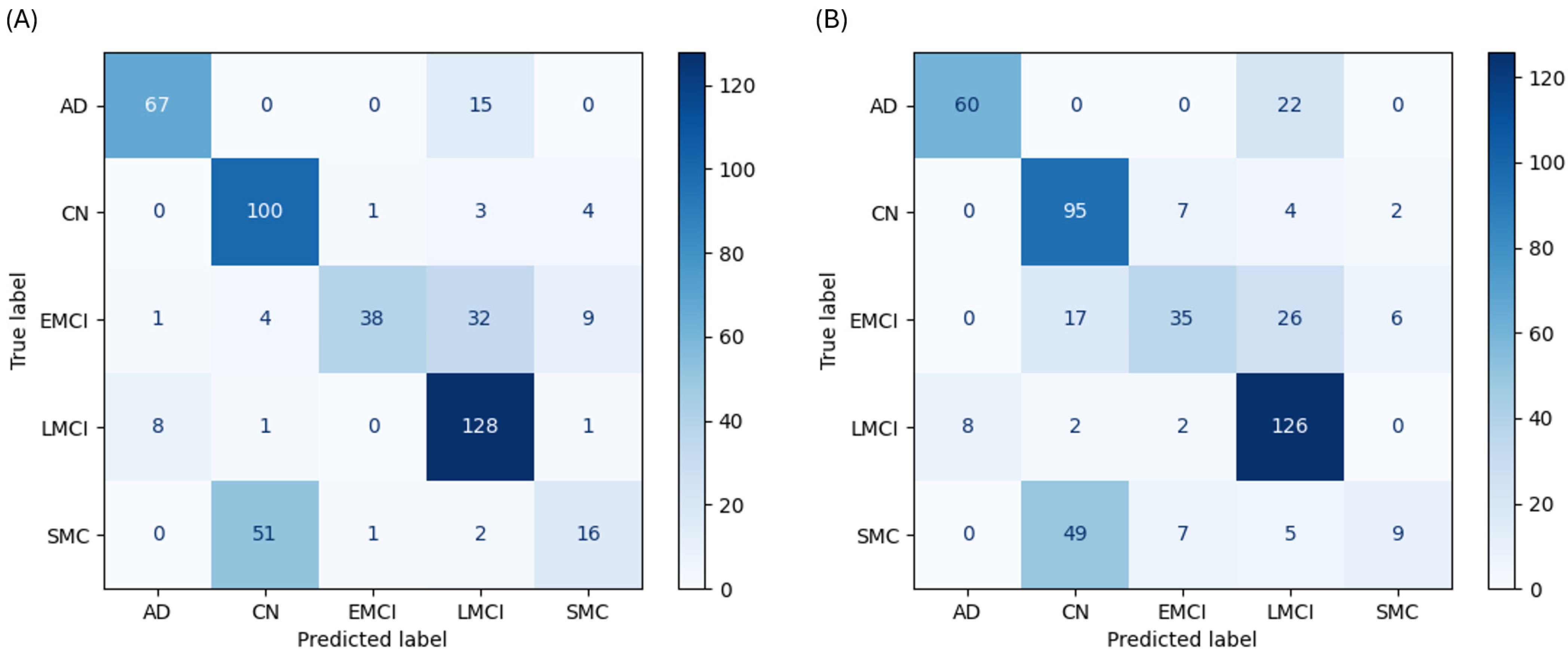
As a linear baseline, the LR model’s performance clearly illustrates the difficulty of separating these clinical states, especially where class boundaries overlap. With cognitive data, the LR model achieved 72.4% accuracy. It was effective at identifying anchor classes, with a recall of 81.7% for AD and 92.6% for CN. However, its performance on ambiguous classes was poor; recall for the SMC class was only 22.9%, with the model misclassifying 51 of 70 SMC cases as CN (Figure 2A). Without cognitive data, its accuracy dropped to 67.4% (Figure 2B).

Figure 2. Confusion matrixes for the logistic regression model on the held-out test set with cognitive assessments (A) and without cognitive assessments (B).

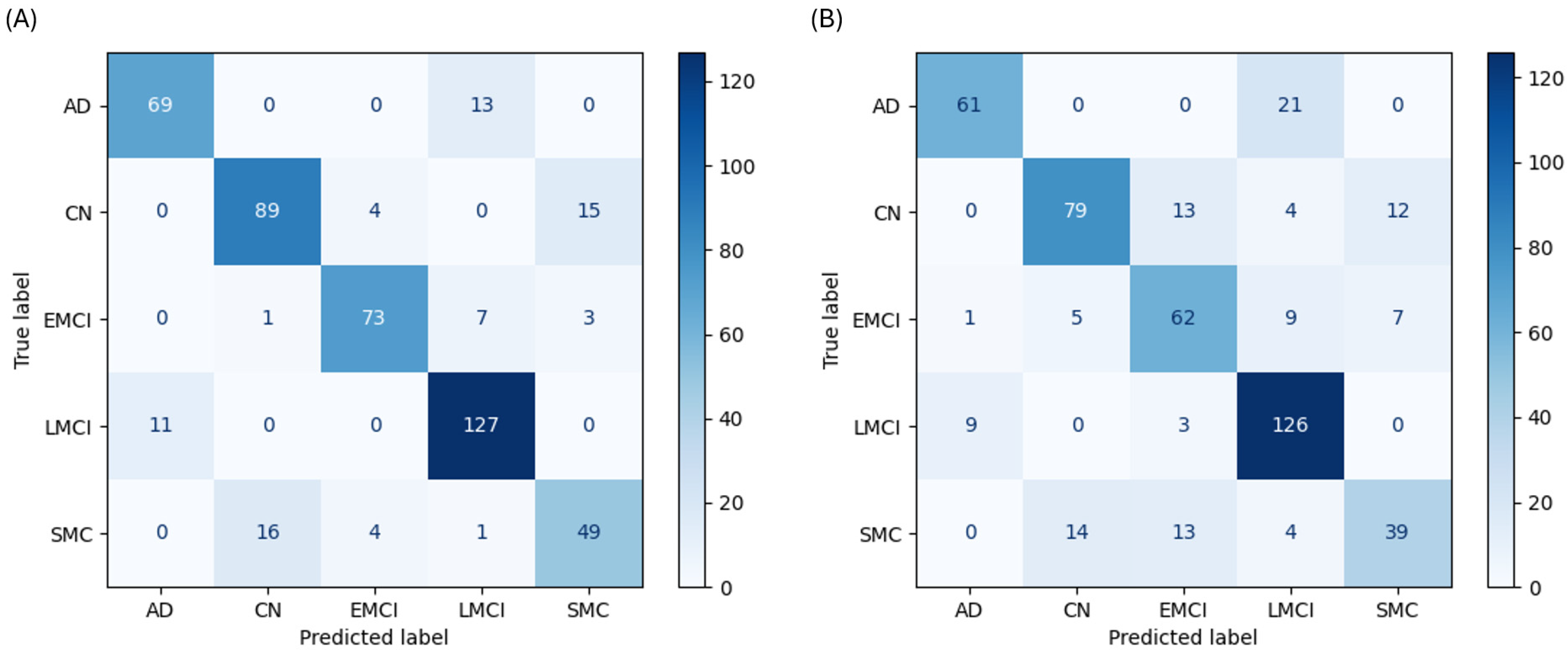
The RF classifier emerged as the most powerful and well-balanced model. With cognitive data, it achieved 84.4% accuracy and demonstrated high, consistent F1-scores across all classes: AD (0.852), CN (0.832), EMCI (0.885), LMCI (0.888), and SMC (0.715). The confusion matrix shows a strong diagonal with high true-positive rates for all classes (Figure 3A). Even without cognitive assessments, the RF model led all others with 76.1% accuracy (Figure 3B).

Figure 3. Confusion matrixes for the random forest model on the held-out test set with cognitive assessments (A) and without cognitive assessments (B).

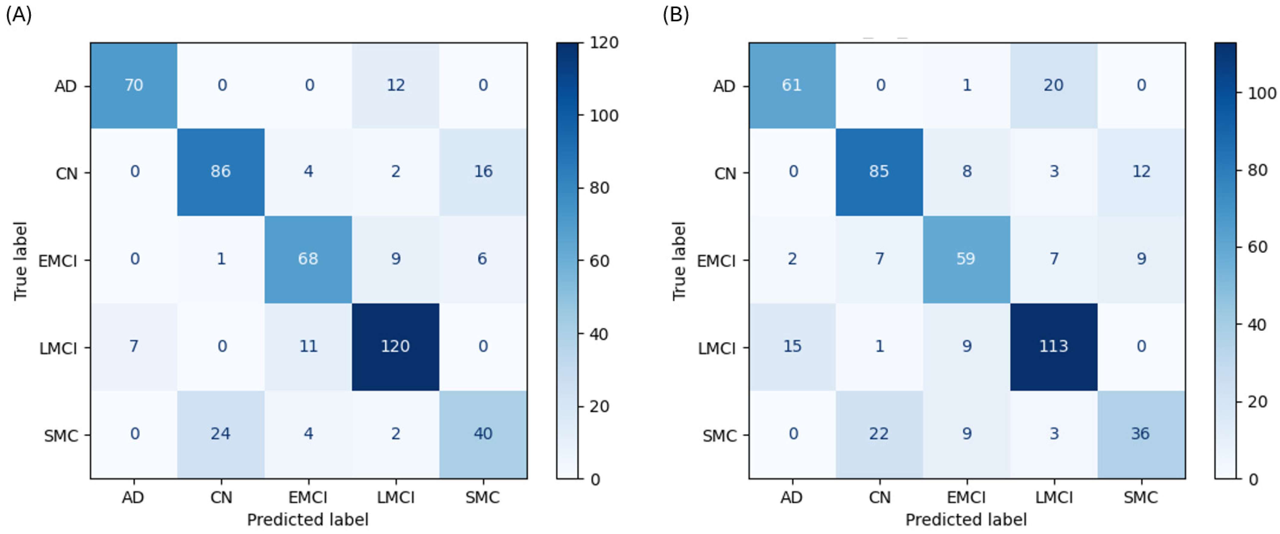
The SVM performed as a strong contender, though its performance revealed specific weaknesses in handling classes with subtle distinctions. The SVM achieved the second-highest accuracy at 79.7% with cognitive data. It performed well on AD (F1-score 0.881) and LMCI (F1-score 0.848) and showed high recall for the populous CN (79.6%) and LMCI (87.0%) classes. However, its recall for the SMC class was 57.1%, misclassifying 24 of 70 cases as CN (Figure 4A). Without cognitive data, its accuracy was 73.4% (Figure 4B).

Figure 4. Confusion matrixes for the support vector machine model on the held-out test set with cognitive assessments (A) and without cognitive assessments (B).

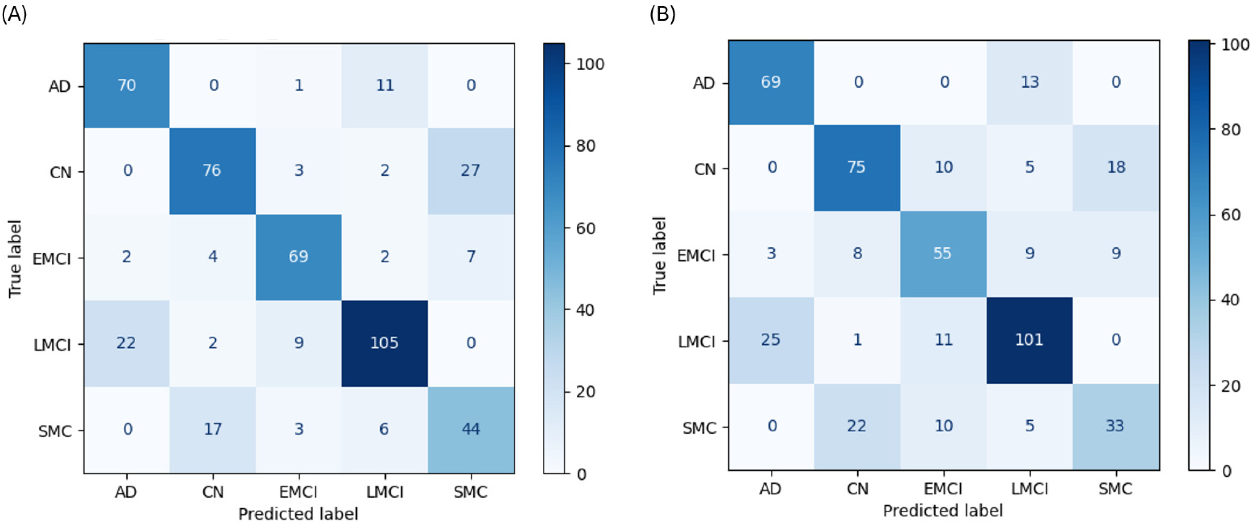
The FNN demonstrated strong but nuanced performance, highlighting the unique learning patterns of a deep learning architecture. With cognitive data, the FNN achieved 75.5% accuracy and produced the highest recall of any model for the AD class (85.4%). Its performance was hampered by a low F1-score for SMC (0.595), misclassifying 17 SMC cases as CN (Figure 5A). Without cognitive data, its accuracy was 69.1%. In this scenario, it had a uniquely high recall for CN (69.4%) but misclassified 25 LMCI cases as AD (Figure 5B).

Figure 5. Confusion matrixes for the feed-forward neural network model on the held-out test set with cognitive assessments (A) and without cognitive assessments (B).

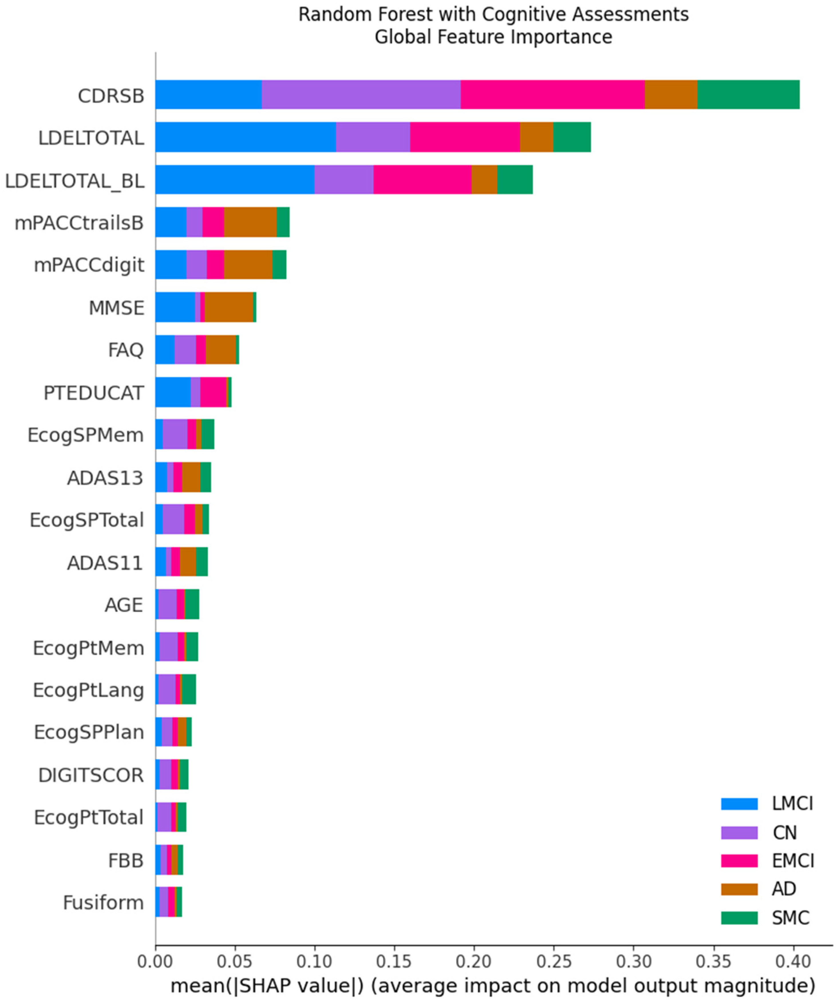
SHAP analysis provides a coherent explanatory picture that differs logically and dramatically between the two feature regimes, revealing why the models make their decisions. When cognitive assessments are included, the feature importance landscape is unequivocally dominated by cognitive scores across all model types. 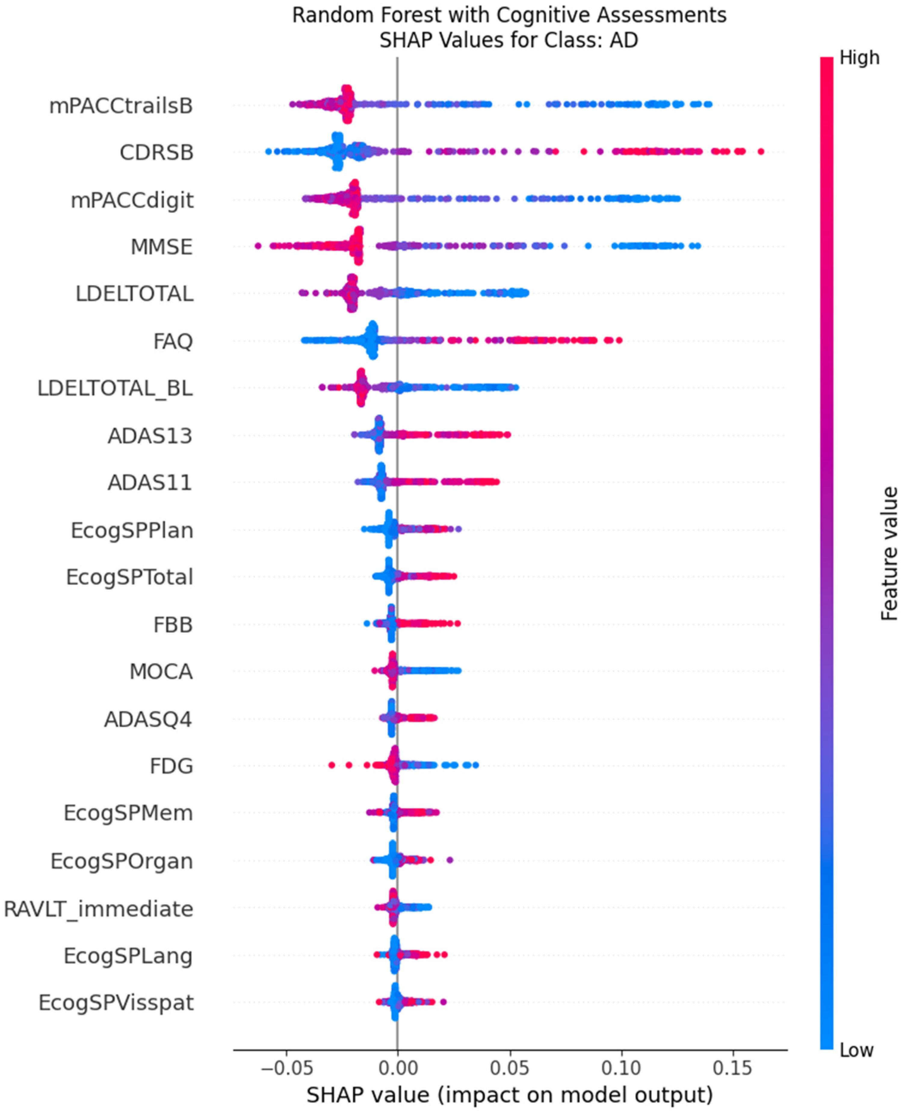For the top-performing RF model, the Clinical Dementia Rating Sum of Boxes (CDRSB) and Logical Memory Delayed Recall (LDELTOTAL) are overwhelmingly the most influential variables, with mean SHAP values far exceeding any other feature (Figure 6). The beeswarm plots confirm this at the instance level; for the AD class, high values of CDRSB (indicating greater impairment, colored red) consistently push the model’s prediction strongly positive, while low values (blue) push it negative (Figure 7). This provides a transparent and clinically intuitive explanation: the models learn to associate poor performance on key memory and functional tests directly with an AD-spectrum diagnosis.

Figure 6. Global feature importance for the Random Forest model with cognitive assessments.

Figure 7. SHAP beeswarm plot for the AD class using the Random Forest model with cognitive assessments.

When cognitive assessments are excluded, the models are forced to recalibrate their decision policies entirely, relying on a combination of imaging biomarkers and demographic features. In this scenario, the most influential predictors become markers of neurodegeneration. 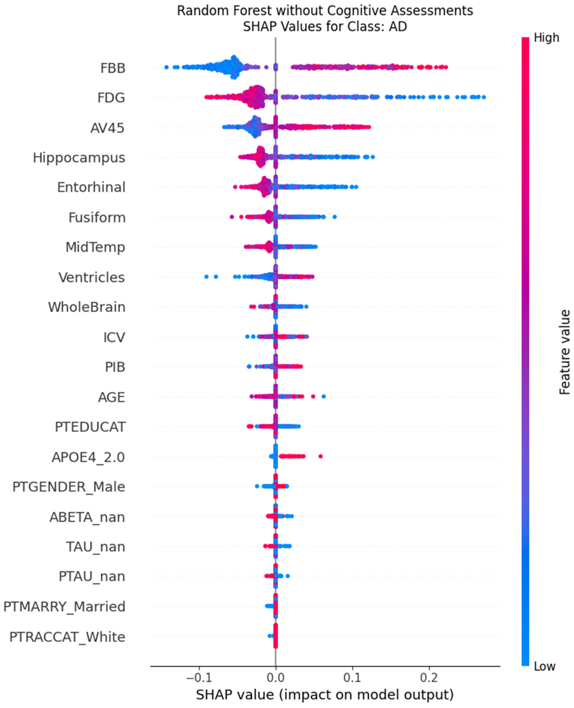For the Random Forest model, PET biomarkers (FBB, AV45, FDG) and MRI volumetrics (Hippocampus, Entorhinal) rise to the top of the importance hierarchy, alongside the patient’s age (Figure 8). The SHAP beeswarm plot for the AD class (Figure 9) elegantly illustrates this shift in logic. It shows that low values (blue dots) for hippocampal volume push the prediction towards AD (positive SHAP values), while high values (red dots) push it away. This aligns perfectly with established neuropathology, where hippocampal atrophy is a well-known hallmark of Alzheimer’s disease.

Figure 8. Global feature importance for the Random Forest model without cognitive assessments.

Figure 9. SHAP beeswarm plot for the AD class using the Random Forest model without cognitive assessments.

4. Discussion

This study’s findings unequivocally demonstrate that cognitive assessment scores are the most powerful predictors for the machine learning-based classification of AD and its precursor stages. The dramatic degradation in performance observed when these functional measures were excluded, with the top-performing model’s accuracy falling from 84.4% to 76.1%, underscores the indispensable role of neuropsychological testing in accurately staging cognitive decline. While biological markers provide an essential foundation, the functional impairment captured by cognitive assessments is paramount for achieving diagnostic precision with computational models.

A central contribution of this work is the use of XAI to move beyond predictive accuracy and provide crucial transparency into the models’ decision-making processes. The application of SHAP confirmed that the models learned clinically intuitive and valid patterns from the data. When available, functional metrics such as the CDRSB and memory recall tests like LDELTOTAL overwhelmingly dominated the models’ logic, confirming that a patient’s ability to perform cognitive tasks is the most salient feature for classification. This contrasts with prior “black box” approaches that, despite high accuracy, offered no insight into their reasoning, limiting clinical trust and applicability.

In the absence of cognitive data, the models intelligently pivoted to a biological signature of AD. Delving deeper into the biomarker-driven model, the top features represent the core pathological tenets of the disease. PET tracers that quantify amyloid plaque burden (FBB, AV45) and cerebral glucose metabolism (FDG) rose to the top of the feature importance hierarchy. The models correctly learned to associate high amyloid burden and low glucose metabolism with an increased likelihood of an AD diagnosis. Similarly, structural MRI features indicating atrophy, such as a smaller Hippocampus and Entorhinal cortex volume, were also learned as significant predictors. This analysis confirms that the “no-cognition” model is not a random guesser but a rational agent that successfully learned the fundamental biological and structural signatures of AD from the data, validating its logic against established neuropathology.

The superior performance of the Random Forest classifier likely stems from its ensemble architecture, which is adept at capturing the complex, nonlinear interactions inherent in the data and is less prone to overfitting than a single deep network might be. A detailed analysis of the error structure across all models reveals the inherent challenges of applying discrete labels to a continuous disease process. The most persistent error was the misclassification of SMC as CN, evident in the low recall for the SMC class. This suggests that the captured features may be insufficient to reliably separate subjective complaints from objective cognitive performance. Furthermore, without cognitive data, all models struggled to differentiate EMCI from its adjacent classes, indicating that biological data alone may lack the resolution to parse subtle, transitional disease stages.

The robustness of these findings is supported by key methodological choices, particularly the use of class weights to mitigate the effects of the imbalanced class distribution present in the dataset. Without this correction, the models would have been heavily biased toward the more populous CN and LMCI classes, further obscuring the true performance on rarer diagnostic groups.

While this study provides valuable insights, its cross-sectional design, using only baseline data, is a key limitation. Future research should prioritize longitudinal modeling to capture disease progression and transitions between stages over time. Such models could offer predictive power not only for current diagnosis but also for a patient’s future trajectory. Furthermore, integrating additional data modalities, such as detailed CSF analytics, emerging blood-based biomarkers, or more advanced model architectures, could enhance accuracy, particularly in the ambiguous early stages of the disease. Ultimately, this work demonstrates that the synergy between high-performing models and robust XAI methods holds immense promise for developing the next generation of clinical decision-support tools that are not only accurate but also transparent and trustworthy.

5. Conclusions

By evaluating four machine learning architectures, this study highlights the inherent challenge of applying discrete classification labels to the AD continuum. Our findings confirm that cognitive assessment scores are the most powerful predictors for this task, with a Random Forest model achieving the highest accuracy at 84.4%. The central contribution of this work is demonstrating that an XAI approach can provide clinically valid insights into a model’s logic. SHAP analysis revealed that the models intelligently pivoted from relying on functional performance metrics to the core biological signatures of AD, such as amyloid burden and hippocampal atrophy, when cognitive data was absent. This synergy between predictive accuracy and validated, transparent reasoning is a crucial paradigm for developing the next generation of trustworthy clinical decision-support tools.