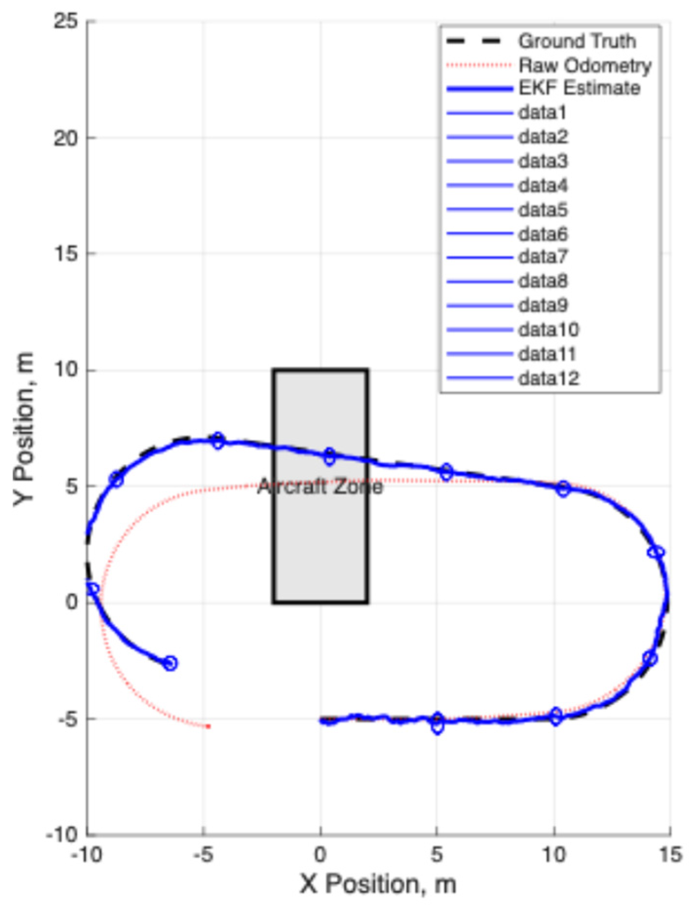
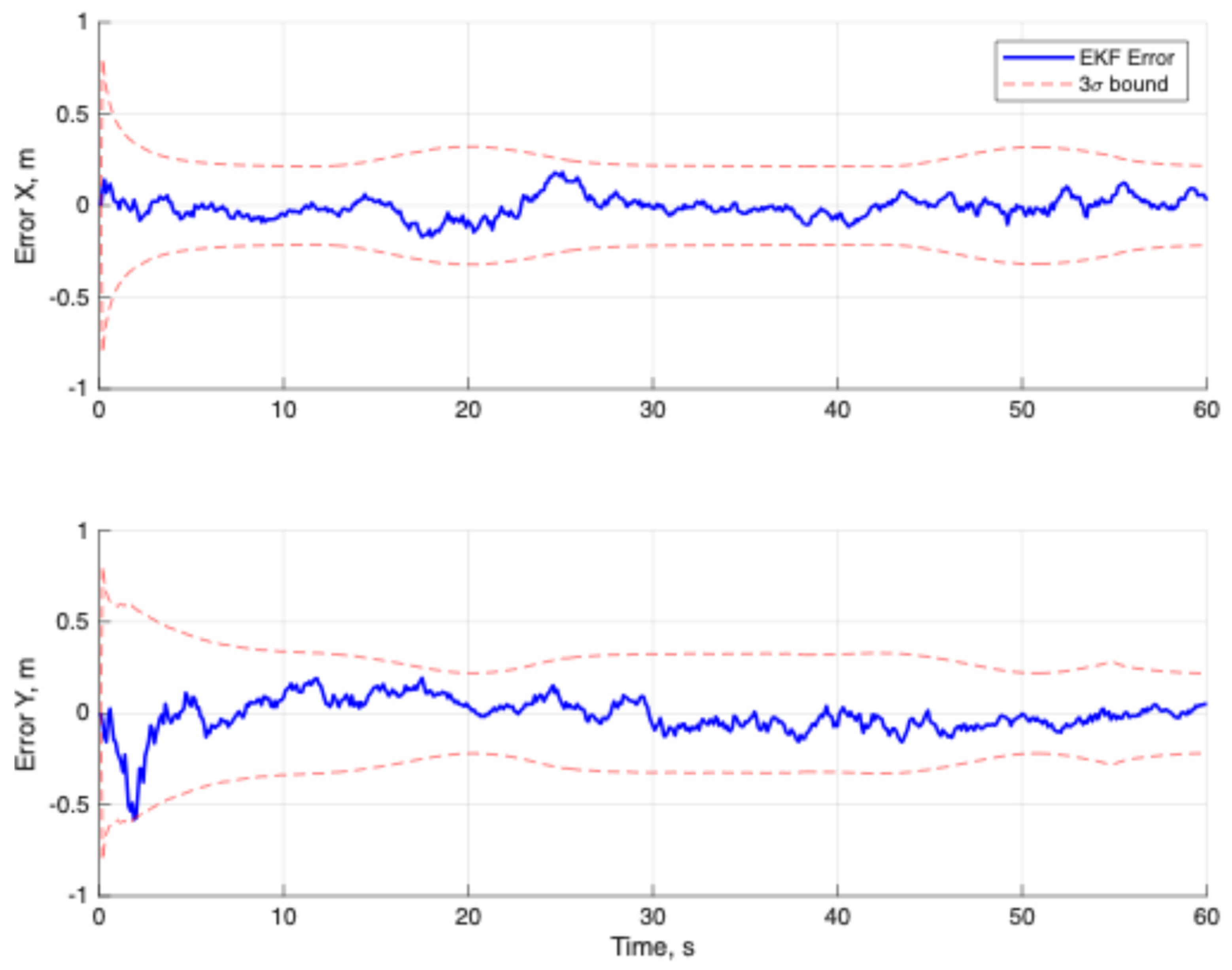
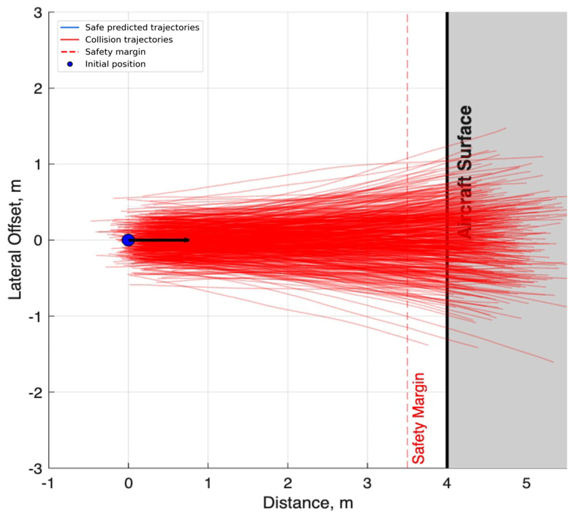
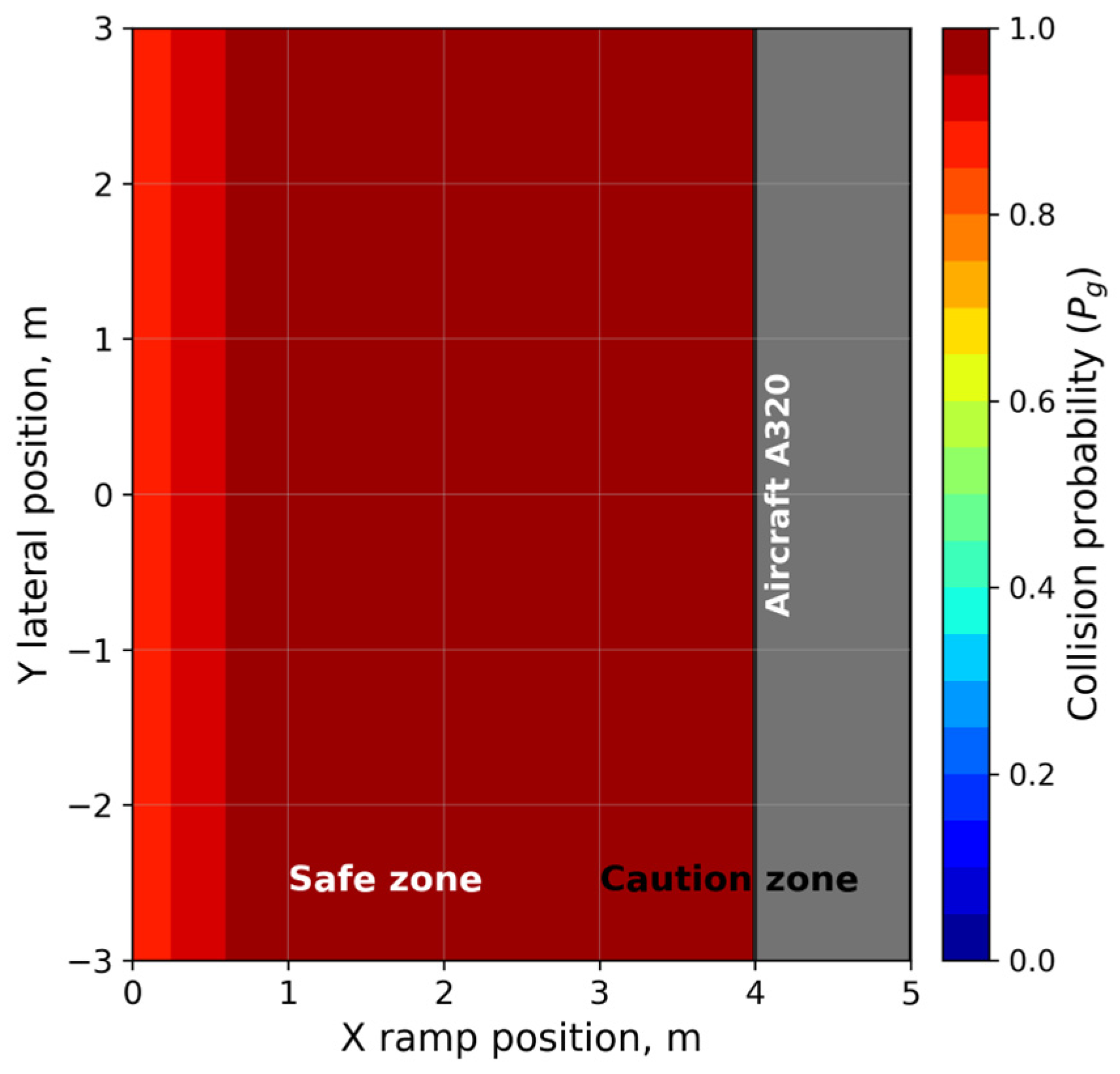
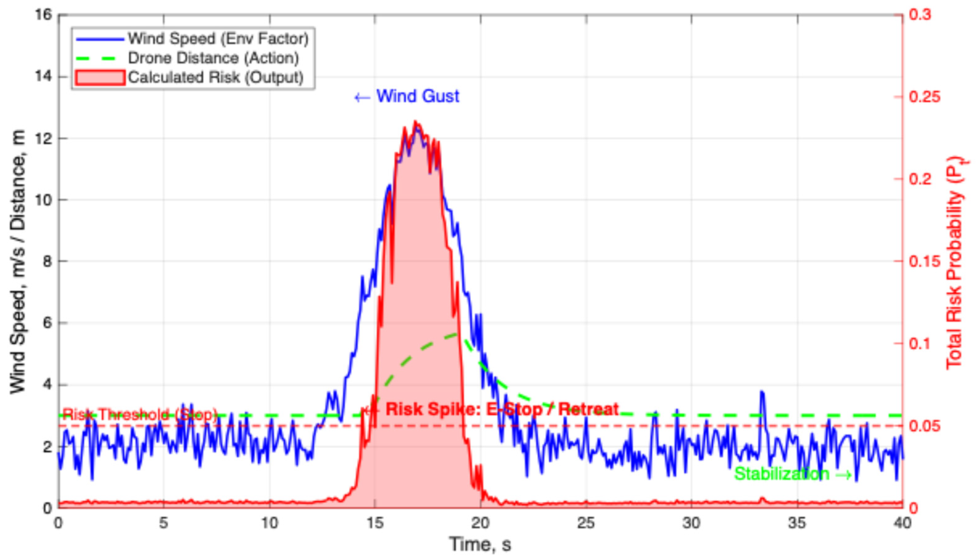
In this study, the term “heterogeneous robotic system” describes the ability of a risk assessment system to process robot state vectors, motion models, sensor uncertainties, and contextual reliability factors. This assessment is demonstrated for two platforms: an unmanned ground vehicle (UGV) with differential drive and an unmanned aerial vehicle (UAV) capable of hovering. Applying this framework to other robotic systems would require the adaptation of the motion model, assessment of measurement noise and collision zones, consideration of aircraft geometry, Bayesian network topology, and risk thresholds. Thus, the research results are transferable at the architectural level; however, their effectiveness is confirmed by evaluating all autonomous airport systems.
2.1. State Assessment and Uncertainty Modeling
The UGV was modeled as a system with differential drive and nonholonomic constraints. The state vector
comprises the Cartesian coordinates (
) and heading angle
:
The control vector
comprises the linear velocity
and angular velocity
. Thus, the UGV state for time step
can be discretely modeled as follows:
where
is white Gaussian noise.
The UGV motion model should ensure that the airport apron work area has a level surface. This assumption is reasonable because airport aprons are typically constructed of asphalt concrete. However, the model does not explicitly account for wheel slippage, surface unevenness, apron contamination, or slope changes. These factors can affect odometry drift and expand the covariance matrix used in subsequent Monte Carlo simulations. Therefore, the parameters of these noises are experimentally determined before practical application [
30].
UAVs used for aircraft maintenance are often quadcopters operating in hovering or low-speed flight modes. The UAV was modeled as a simplified system with six degrees of freedom, which was converted to a state vector comprising the position (
) and yaw relative to the aircraft
:
The control vector was specified by setting the velocities in the local coordinate system:
. Thus, the UAV state for time step
can be discretely modeled as follows:
The EKF performs a two-stage process at each step
. The first stage is to predict a robot’s state using an a priori estimate:
The a priori covariance matrix of errors is estimated as follows:
where
is the Jacobian of the state transition function (
) at point
. The Jacobian for a UGV is given as follows:
The second stage involves correcting the predicted state based on the received
measurement data. The updated state is represented as follows:
where
is the observation matrix,
is the measurement noise covariance, and
is the Kalman gain.
The EKF outputs the posterior covariance matrix
, which helps determine the shape and orientation of the uncertainty ellipsoid around a robot’s position in space [
31]. The numbers (
) and vectors of the matrix (
) determine the length of the semi-axes and the inclination angle of the uncertainty ellipsoid. The distribution
serves as an input parameter for the Monte Carlo simulations used to generate the probabilistic trajectories.
2.2. Prediction of the Collision Probability
Given the density of obstacles on the airport apron and their complex geometry, probabilistic calculations using a Gaussian distribution are ineffective. In such a dynamic environment, Monte Carlo simulations allow for an effective risk assessment [
32] by generating a set of robot trajectories over a given time horizon
.
The estimated state and covariance obtained by the EKF can be used to generate an array of states . The standard approach for Monte Carlo simulations uses an adaptive number of simulations. In this study, a fixed number of simulations ( = 10,000) was used to identify risks with high reliability. The number of simulations was set to ensure the coverage of unlikely scenarios that arise during robot maneuvers or changes in sensor readings.
The quantitative sample size for the Monte Carlo simulation was selected through sensitivity analysis. During the experiments, 2000–15,000 simulations were conducted. For a sample of 3000 simulations, the collision probability demonstrated a high scatter of results and low tail sensitivity. Analysis of a sample of 8000 events revealed a relatively low error, which was also maintained for 15,000 simulations, but with increased computational complexity. Therefore, the authors believe that a sample size of 10,000 simulations provides an optimal compromise between all the necessary model parameters.
The initial state vector is generated as follows:
where
is a
matrix with a sample of random variables
and
is the Kronecker product.
The EKF state estimate is used to fit the local uncertainty of the state of the robot to a Gaussian distribution. In the next step, the Monte Carlo simulation propagates these states through the collision geometry and nonlinear motion models. The trajectories contain nonlinear dispersion and boundary effects that are difficult to describe analytically. However, the current study is limited by global navigation satellite system (GNSS) multipath and lidar reflections from the aircraft’s metalized surfaces, which require calibration.
Calculating 10,000 predicted trajectories
requires substantial computational resources. The prediction task was parallelized on a graphics processing unit (GPU) to allow for real-time risk assessment. Thread
independently calculates the state vector evolution as follows:
This parallelization allows the prediction task to be performed in <20 ms for 10–50 Hz control frequencies.
A detailed risk map is created, and each point of a trajectory is checked for the risk of collision with the aircraft. The collision function for the
-th trajectory is calculated as follows:
The final probability is calculated as follows:
Using a sample of 10,000 simulations helps introduce a highly granular gradation to the risk assessment, allowing the proposed model to effectively classify potential threats. For example, 10,000 simulations may result in five potential collisions, causing the model to proactively reduce the speed of the UGV. In contrast, 500 simulations run under the same conditions may identify a zero risk, which can cause the model to assume a false sense of safety.
The model applies the law of large numbers to reduce the probability
to the true probability
. The estimation standard error helps provide information on the model accuracy and is calculated as follows:
The number of Monte Carlo simulations was set to 10,000 to balance the computational complexity with the need to identify critical collision scenarios, which are relatively rare under real-world conditions [
33]. Several experiments were conducted while varying the number of simulations to determine the specific number of simulations. The estimated collision probability exhibited high variance and low sensitivity to tail events with 3000 simulations. The increase in model accuracy was negligible with 15,000 simulations, but the computational costs were high. Experiments were also conducted with 2000–15,000 simulations to test the stability of the estimated collision probability. The estimation error was less than 5% with 8000 or more simulations, which is sufficient for decision-making when a robot is in a critical area of the airport apron.
2.3. Contextual Analysis on System Reliability
The geometric collision probability
is suitable for scenarios in which the UGV and UAV operate normally. However, in real-world scenarios on airport aprons, external stochastic factors, including wind gusts, precipitation, and electromagnetic interference, affect the reliability of autonomous mobile robotic systems. A Bayesian network was used to integrate these factors into a single risk metric [
34].
Two specialized network topologies were constructed for the UAV and UGV using distributed acyclic graphs. Each network had identical structures, including the root, intermediate, and leaf nodes. The root nodes comprised the wind speed (), GNSS signal quality (), and illumination level in the inspection zone (). The intermediate nodes included visual odometry errors, which are directly dependent on (i.e., system accuracy decreases in bright light and at night), and position-holding stability, which depends on and . The leaf node represents the probability of system failure (), which implies that the UAV and UGV exit the inspection zone. The main difference between the network topologies was that the UGV network accounts for the coverage of the inspection zone and the density of dynamic obstacles.
Environmental disturbance effects are represented as additional constraints that affect localization, perception, and route selection reliability within the extended model. GNSS multipath effects are represented in the model as position measurement bias. LiDAR distortions are modeled as noise variance in ranging and as periodic spikes in measurements. Noise enhancement in the UGV motion model represents contamination and wheel slip associated with the operating surface. Personnel and ground vehicle movements are modeled using dynamic obstacle density nodes in a Bayesian network and moving obstacle trajectories in the Monte Carlo prediction layer. These effects were not calibrated using real sensor data in this study. As a result, the previously described disturbance parameters are interpreted as constraints at the robustness analysis scenario level.
Table 1 presents the modeling constraints and their impact on the proposed model.
Table 2 presents the structure of the Bayesian network. In this study, the Bayesian network does not replace the geometric collision model. It represents a contextual reliability layer for increasing the assessed risk level when external conditions reduce confidence in localization and perception processes. Node states were divided into three layers to maintain computational efficiency and support real-time updates. UAV and UGV networks have similar logic, but the UGV network also considers the dynamic density of obstacles and the coverage of the inspection zone, as this type of robot interacts with ground equipment and personnel [
35].
The probability of system failure for the stability node (
) is calculated as follows:
This procedure is required to dynamically update the estimated system reliability. The probability at node W changes with increasing wind speed, which causes the probability signal to propagate throughout the model and ultimately increase the final value of
. In this study, a conditional probability table (CPT) [
36] was constructed based on expert judgment from ground handling personnel and aircraft inspection specialists along with statistics on sensor and navigation system failure. Expert data were used to initialize the Bayesian network and define a priori distributions, while simulations of standard sensor degradation scenarios and environmental disturbances were used to refine the numerical probability values. This hybrid approach has found wide application in reliability analyses of complex systems where real operational data are limited and ensures model reproducibility while maintaining adaptability.
In this study, the use of CPT is justified because operational data for autonomous automated systems interacting with aircraft have not yet been generated. Additional experiments were conducted to reduce the subjectivity of CPT and refine the simulation scenarios that simulated sensor degradation, wind interference, and localization. Furthermore, sensitivity analyses of CPT were conducted. The robotic system’s performance remained unchanged, demonstrating the robustness of the decision-making process.
The CPTs were formalized through a structured expert procedure to ensure a high level of reproducibility of the Bayesian reliability level. This expert group included representatives of the Kazakh aviation industry with practical experience in ground handling, aircraft inspection, and aviation safety risk assessment. Each expert independently assigned probabilities to each node of the Bayesian network using a three-level linguistic scale, including low, medium, and high levels of degradation. These assessments were converted into numerical probability intervals.
The weight of the expert assessment
correlates with the expert’s area of expertise, his work experience, and indicators of agreement among all experts:
where
is the normalized expert assessment, and
the number of experts who participated in the assessment. The aggregated entry in the CPT is then calculated as follows:
Inter-rater agreement is assessed by checking monotonicity constraints. CPT entries for the monotonicity rule are fed back into the model for re-evaluation by experts. The uncertainty in CPT values is propagated by varying the CPT values within intervals of and , followed by repeated Bayesian inference. The decision outcome is robust if the risk class does not change under these recalculations.
This procedure is necessary to ensure the model’s objectivity, thereby making CPTs transparent, reproducible, and verifiable. In cases where a large dataset is missing, the proposed CPTs, derived from expert judgment, serve as engineering a priori conditions necessary for future updates until empirical data becomes available.
Table 3 presents the CPT identification protocol.
In traffic safety management models, the integrated risk
is defined as the conditional probability of an incident
occurring on the forecast horizon
:
In this study, the incident
was defined as an integrated vector of several events: the collision probability
over the time interval
estimated from the trajectories obtained by Monte Carlo simulations and the critical failure probability
obtained by the Bayesian network. If these probabilities are assumed to be independent for a fixed
, the integrated risk can be defined as follows:
The assumption that and are independent only applies to fixed robot states and short-term planning intervals. In Equation (18) represents the geometric probability of the predicted robot trajectories and aircraft boundaries’ intersection. Furthermore, is the contextual probability of system reliability degradation due to wind, GNSS signal quality, lighting, or sensor uncertainties. These probabilities may be correlated in real airport conditions because external disturbances and sensor degradation can simultaneously affect and . Consequently, the independence formulation is interpreted as a mathematical approximation rather than a universal equality.
A conservative upper-bound formulation is used to ensure safe operations, in which the correlation between and cannot be excluded. This formulation helps to prevent risk underestimation and is directly consistent with conservative engineering practice. This study uses an independence-based expression, and the conservative bound is primarily needed for future practical implementation.
For a fixed system state
,
and
were assumed to be independent to facilitate real-time risk assessment. These probabilities are partially correlated under real-world conditions because of the effects of sensor degradation and external environmental effects on system operation. If independence is not guaranteed, a conservative upper bound can be used as follows:
This ensures that the robotic system complies with safety-critical practices and helps ensure a safety margin during decision-making in the airport apron adjacent to the aircraft [
37]. In this study, a threshold risk of
= 0.05 was applied, which corresponds to the conservative engineering approach adopted for safety-critical systems [
38] and ALARP logic [
39]. If
, risk mitigation measures must be implemented. Note that
is an acceptable level of risk within the interval
and does not represent the actual incident frequency. Numerical simulations revealed that the number of false alarms increased up to a threshold of
= 0.03. At
≥ 0.08, a response delay occurred in the dynamic operating scenarios. Therefore, the selected threshold balances operational efficiency with the effective monitoring of robotic navigation safety.
The threshold value was selected through sensitivity experiments. For threshold values below 0.03, the model begins to generate false alarms, resulting in the abortion of the verification task even though the robot was outside the collision zone. For threshold values above 0.08, the system begins to lag in dynamic scenarios, reducing the safety margin. Therefore, = 0.05 was chosen as a conservative compromise between continuous operation and safety. This value is not interpreted as a tolerance for accident frequency but rather as a decision threshold for the risk assessment system to trigger preventive actions.
Independence is used only as a first-order approximation for a fixed-state estimate. The geometric event
, which is represented by the intersection of the predicted trajectory and the aircraft boundary, and the system reliability degradation event
, which is a contextual system failure, are conditionally independent for the current estimated state
:
The model assumes that this assumption does not hold for all airport apron conditions. For example, if the GNSS signal degrades, the trajectory variance increases simultaneously, and the probability of Bayesian failure increases. Consequently, the risk assessment, considering independence, underestimates the risk in cases where the disturbance affects both layers. To avoid unsafe underestimation, a conservative layer merging bound can be achieved:
This study uses independence metrics and nominal simulation scenario metrics. A conservative upper-bound formulation is recommended for scenarios with deterioration or correlated disturbances.
The risk
of an incident is adjusted by the severity of its consequences
, which depends directly on the position of the robotic system relative to the critical zones of an aircraft:
Based on the calculated
R, the proposed model decides the action of the robotic system according to the reaction matrix presented in
Table 4.