Article

Coupling 3D CFD of Air Knife Jets with an Analytical Model for Coating Thickness Prediction and Operating Window Definition in Hot-Dip Galvanizing


1
Australian Research Council (ARC) Industrial Transformation Training Centre (ITTC) for Innovative Composites for the Future of Sustainable Mining Equipment, University of Wollongong, Wollongong, NSW 2522, Australia
2
School of Engineering, University of Wollongong, Wollongong, NSW 2522, Australia
3
HBIS Materials Technology Research Institute, Shijiazhuang 050023, China
4
China-Serbia Belt and Road Joint Laboratory on Green Steel Manufacturing, Shijiazhuang 050023, China
5
Changshu Everbright Material Technology Co., Ltd., Suzhou 215500, China
*
Authors to whom correspondence should be addressed.
Eng 2026, 7(5), 206; https://doi.org/10.3390/eng7050206
Submission received: 20 March 2026 / Revised: 23 April 2026 / Accepted: 26 April 2026 / Published: 29 April 2026
(This article belongs to the Section Materials Engineering)

Abstract

A coupled modeling framework is developed to predict coating thickness after air knife wiping in hot-dip galvanizing. A 3D large eddy simulation (LES) using the WALE sub-grid scale (SGS) model is performed to resolve the jet impingement on the moving strip. Time-averaged wall static pressure p ω y and wall shear stress τ ω y along the strip direction are extracted and used as driving inputs for a thin film model. Starting from the continuity and momentum equations, a lubrication-type formulation is derived, leading to a local cubic equation for film thickness h ( y ) that accounts for both pressure gradient and gravity. A coupling workflow is established to preprocess the LES wall signals and compute the final coating thickness h f i n a l . Parametric sweeps of inlet total pressure P 0 and the knife-to-strip distance H are employed to construct operating window maps. The predicted trends show that increasing P 0 or decreasing H intensifies wall loading and reduces h f i n a l , while the operating window boundary is governed by the balance between the gas-induced shears. Representative results, including peak wall loading and thickness ranges, are reported for industrially relevant operating conditions.

1. Introduction

Hot-dip galvanizing is widely used to provide corrosion protection for steel strips [1,2]. In a continuous galvanizing line, the final coating thickness is primarily controlled by air knife wiping, where high-speed jets impinge on the moving strip and remove excess molten zinc [3,4,5]. Accurate thickness control remains challenging because the gas jet produces strong pressure gradients, intense surface shear, and complex 3D flow structures near the impingement and wall jet regions [6,7,8,9,10], as schematically illustrated in Figure 1. In practice, unstable wiping can also introduce surface defects and nonuniformities that are undesirable for downstream forming and painting [11].
Existing approaches for coating thickness prediction can generally be divided into computational fluid dynamics (CFD)-based analyses and simplified thin film models [12,13,14,15]. High-fidelity CFD can capture the detailed jet flow physics near the strip, but coating thickness cannot be obtained directly unless a free surface or multiphase formulation is introduced, which significantly increases computational cost and modeling complexity [16,17,18]. In contrast, thin film models are computationally efficient, but their predictive capability depends strongly on the driving inputs, such as the pressure gradient and surface shear stress, which are often simplified, approximated or tuned [14,15,16]. Therefore, there remains a need for a practical modeling framework that can retain the essential 3D gas flow physics while enabling efficient and physically grounded prediction of coating thickness.
In this study, a coupled framework combining 3D CFD results and a lubrication-type thin film model is developed. The 3D CFD simulation resolves the air knife flow and provides time-averaged wall loading in terms of wall pressure p ω y and wall shear stress τ ω y . These quantities are then introduced into the thin film model derived from the continuity and momentum equations, with gravity included, to predict the coating thickness distribution and a representative final thickness [15]. The proposed framework provides an efficient route for linking detailed jet flow characteristics to coating thickness prediction and for constructing operating window maps under different wiping conditions.

2. Numerical Model and Methodology

2.1. Computational Geometry and Boundary Conditions

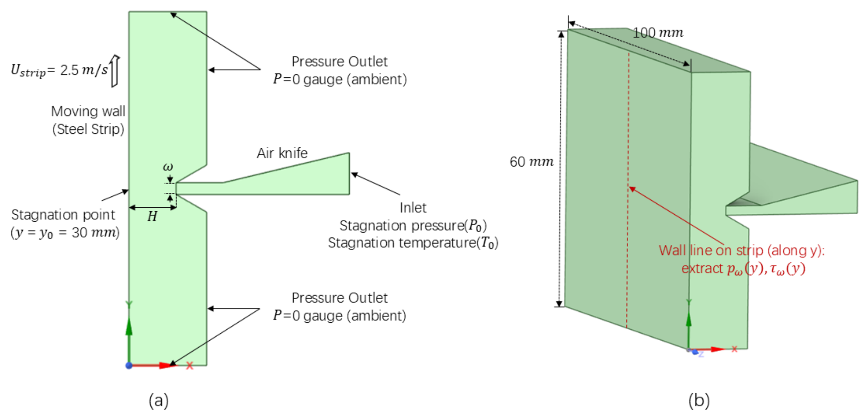
The computational geometry represents the air knife and the moving strip. The strip moves upward along the y direction at U s t r i p = 2.5 m/s. The slot width is ω = 1.5 m m and the knife-to-strip distance is H = 100 m m . The computational domain length and width follow the baseline configuration and are shown in Figure 2. The inlet boundary condition at the slot is specified using inlet total pressure and total temperature ( P 0 , T 0 ). The far boundaries are treated as pressure outlets with p = 0 gauge, consistent with ambient pressure [16]. The stagnation point location is defined at y = y 0 = 30 m m [12]. The wall line used to extract p ω y and τ ω y is defined on the strip surface along the y direction. The selected geometric and boundary settings follow common air knife configurations reported in prior numerical studies [4,9,19,20].

2.2. LES WALE Setup and Numerical Setting

A 3D large eddy simulation is performed to resolve the unsteady jet impingement and wall jet flow [17,21]. The filtered governing equations are solved using the WALE sub-grid scale model to present unresolved turbulence. Spatial discretization uses second-order schemes, with the convection terms in the momentum equations discretized using the bounded central differencing scheme, and pressure–velocity coupling is handled using a PISO-type algorithm [22]. The simulation is advanced in time with a fixed time step t = 5.0 ×   10 7 s. The solution is first advanced until statistical stationarity is reached, after which wall quantities are sampled over a time window T s for time averaging [12,16].

2.3. Grid and Time Setup

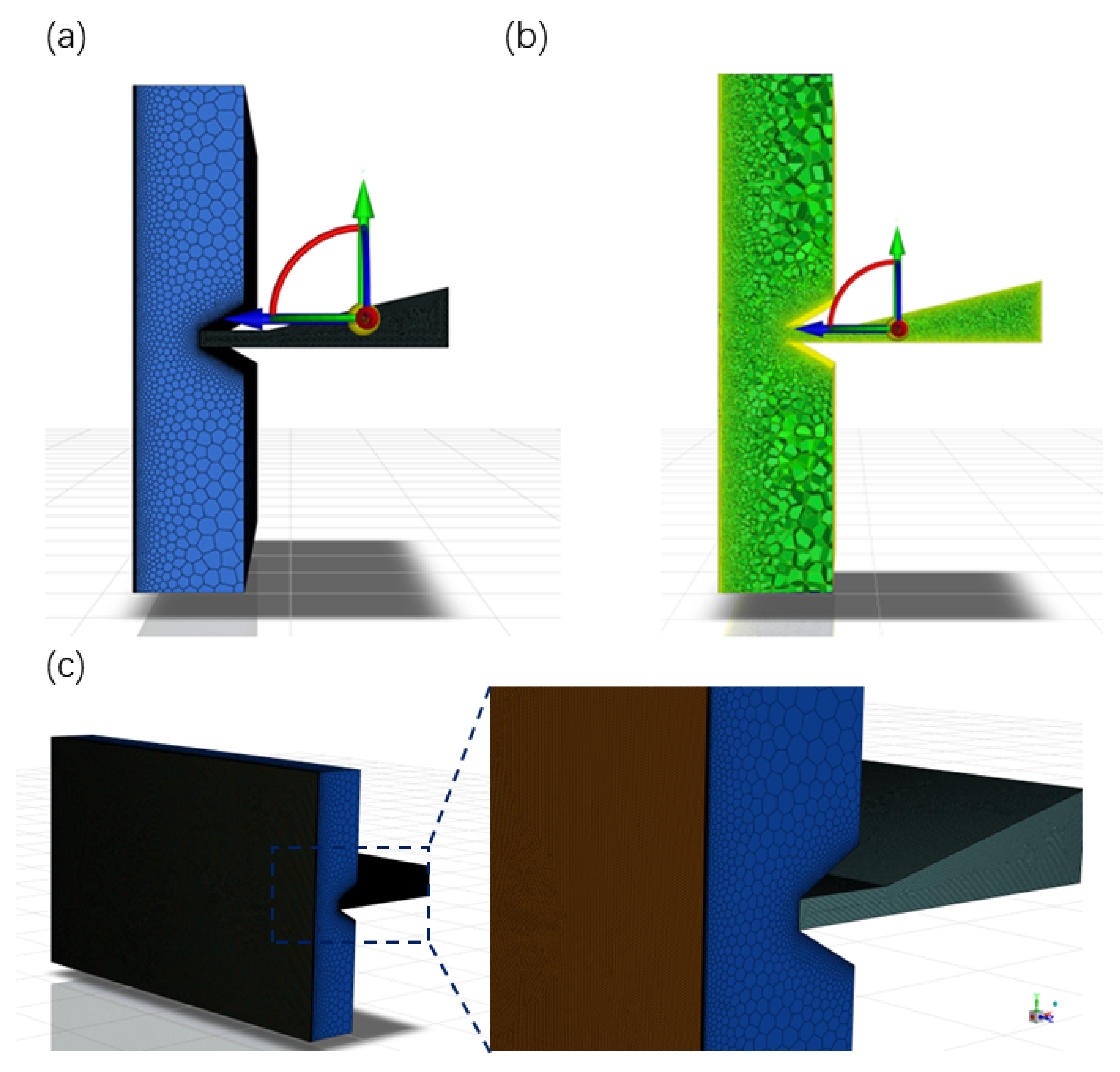
As shown in Figure 3, the computational mesh was generated using Fluent Meshing (ANSYS Fluent 2023 R2, Ansys Inc., Canonsburg, PA, USA) with local size controls applied to the slot exit and the impingement region. The minimum cell size in the refined region was set to approximately 0.1 m m , while the far-field mesh was smoothly coarsened with a growth rate of 1.2 to limit the overall cell count. A polyhedral volume mesh was adopted to improve robustness for the complex jet impingement flow topology. Near the moving strip, boundary layer inflation was applied using a smooth transition with 15 layers and a growth rate of 1.15 to provide adequate near-wall resolution for wall loading extraction [23]. The resulting mesh contains approximately 6.67 ×   10 6 cells, with a minimum orthogonal quality of about 0.20.
The LES was advanced in time using a fixed time step of t = 5.0 ×   10 7   s . This time setup was selected to keep the Courant number within a typical range for LES based on the minimum cell size and the jet exit velocity scale [17]. The simulation was first run until the flow reached statistical stationarity, after which time-averaged wall quantities were collected over a sampling window T s for coupling with the film thickness model. The adequacy of the mesh and temporal sampling is assessed using the mesh sensitivity and sampling checks in Section 4.

3. Model for Predicting the Coating Film Thickness

3.1. Film Thickness Model

We consider a thin liquid coating on a vertically moving strip and predict the steady thickness h ( y ) along the strip direction y (positive upward). The normal coordinate is x , with x   = 0 at the strip wall and x = h ( y ) at the gas–liquid interface. The coating is treated as an incompressible Newtonian fluid with density ρ and viscosity μ . The governing equations are the continuity equation and the y-momentum equation:
u y + v x = 0 ,
ρ u u y + v u x = p y + u 2 u y 2 + 2 u x 2 ρ g ,
where u ( y , x ) and v ( y , x ) are the velocity components along y and x , respectively. We consider a lubrication-type approximation for the post-wiping layer, whose thickness is small relative to the characteristic streamwise length scale. Under this framework, the dominant balance is mainly among pressure gradient, viscous stress, strip dragging, and gravity. Accordingly, film inertia is neglected, 2 u / x 2 2 u / y 2 , and the pressure is assumed to be uniform across the film thickness, so that it varies primarily along the strip direction [14,15], yielding
μ 2 u x 2 = d p d y + ρ g .
The boundary conditions are no-slip at the strip wall and a prescribed interfacial shear stress imposed by the gas [13,23],
u 0 = U s t r i p ,
μ u x x = h = τ ω y .
The pressure in the film is taken as the wall pressure distribution supplied by CFD [12], consistent with the lubrication approximation in which pressure is assumed uniform across the film thickness.
p y = p ω y .
Integrating Equation (3) with Equations (4) and (5) yields
u y , x = U s t r i p + 1 μ τ ω y x + d p ω d y + ρ g x 2 2 h x .
The volumetric flow rate per unit width is
q y = 0 h y u y , x d x = U s t r i p h + τ ω y 2 μ h 2 1 3 μ d p ω d y + ρ g h 3 .
For steady wiping, d q d y = 0 , so q is constant. The model is closed by prescribing q = q 0 , where q 0 represents the incoming dragged film flow without wiping [16]. This serves as a simplified inlet condition for the analyzed downstream region and allows the effect of CFD-derived wall loading on the subsequent thickness evolution to be isolated. Substituting q 0 into Equation (8) gives a local cubic equation for h ( y ) ,
1 3 μ d p ω d y + ρ g h 3 τ ω y 2 μ h 2 U s t r i p h + q 0 = 0 ,
and the physically meaningful thickness is taken as the positive real root.

3.2. Coupling Procedure and Operating Window Definition

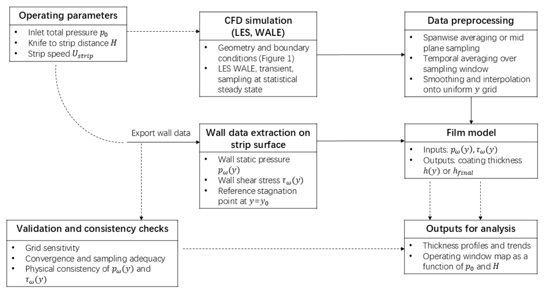
The film thickness model requires the wall p ω ( y ) and wall shear stress τ ω ( y ) along the strip surface. These quantities are obtained from the LES results and serve as the driving inputs for the local cubic equation derived in Section 3.1. The present framework adopts a one-way coupling strategy, in which the gas flow determines the wall loading applied to the liquid film, while the feedback of coating thickness evolution on the gas flow is neglected. This simplification is considered reasonable under the present conditions because the coating thickness is much smaller than the characteristic scale of the air knife flow, and its influence on the overall gas flow structure is therefore expected to be limited. The coupling workflow adopted in this study is summarized in Figure 4 [8,12,14,24].
The wall static pressure p ω ( y ) and wall shear stress τ ω ( y ) are extracted on the strip wall along the y direction, using the stagnation point location y = y 0 as the reference. After the flow reaches statistical stationarity, the extracted signals are time-averaged over a sampling window T s to obtain one-dimensional distributions [17],
p ω ¯ ( y ) = 1 T s t 1 t 2 p ω y , t d t ,
τ ω ¯ y = 1 T s t 1 t 2 τ ω y , t d t .
When required, the time-averaged fields are further averaged in the spanwise direction, or alternatively sampled on the mid-plane, to obtain representative profiles along y . In the present study, the center cross-section is used for the main analysis because it is intended to represent the wiping behavior in the central part of the domain, away from the lateral boundaries. Under the present configuration, lateral edge effects are expected to remain mainly confined to the side regions, while the central region provides the most representative basis for comparing the effects of   P 0 and H . Nevertheless, the possible influence of domain width and widthwise nonuniformity is acknowledged, and a more systematic investigation of truly 3D effects is left for future work. The averaged data are then interpolated onto a uniform y grid [17,25]. The pressure gradient needed by the film model is computed from p ω ¯ ( y ) using finite differences after mild smoothing to suppress high-frequency fluctuations [14,16], for example
d p ω ¯ d y y i = p ω ¯ y i + 1 p ω ¯ y i 1 y i + 1 y i 1 .
With τ ω ¯ y and d p ω ¯ d y , the coating thickness distribution h ( y ) is obtained by solving the local cubic equation from Section 3.1 at each y location and selecting the positive real root. A representative final thickness h f i n a l is defined at a prescribed downstream location, or as an average over a downstream interval, for operating window construction. The above procedure is repeated for different inlet total pressure P 0 and knife-to-strip distance H to obtain thickness trends and the operating window map [25].
The inlet flux q 0 in the film model is treated as a fixed inlet parameter. In the present study, q 0 is set once using a reference operating condition to yield a realistic baseline thickness, and the same q 0 is used for all operating conditions. This treatment is a modeling simplification intended to isolate the influence of the CFD-derived wall loading on downstream thickness evolution when P 0 and H are varied. In a fully coupled system, the actual inlet flux may also vary with operating conditions, and allowing q 0 to vary accordingly would be an important extension for future work.

4. Results and Discussion

4.1. Baseline Flow Feature

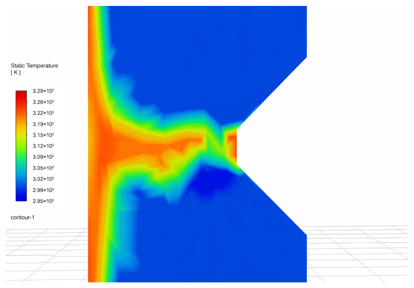
Figure 5 and Figure 6 present the baseline flow field characteristics on the center plane at z = −50 m m . The static temperature contour (Figure 5) highlights the development of the jet from the slot exit, followed by a concentrated impingement region at the strip surface and the formation of a wall jet layer that spreads both upward and downward along the moving strip. The most pronounced temperature gradients are confined to the near-nozzle and impingement zones, where the shear layer around the jet core promotes strong entrainment and mixing with the surrounding ambient air. Away from the jet-affected region, the field becomes nearly uniform, indicating that the thermal disturbance is spatially localized and that the far-field boundaries remain close to the ambient reference state.
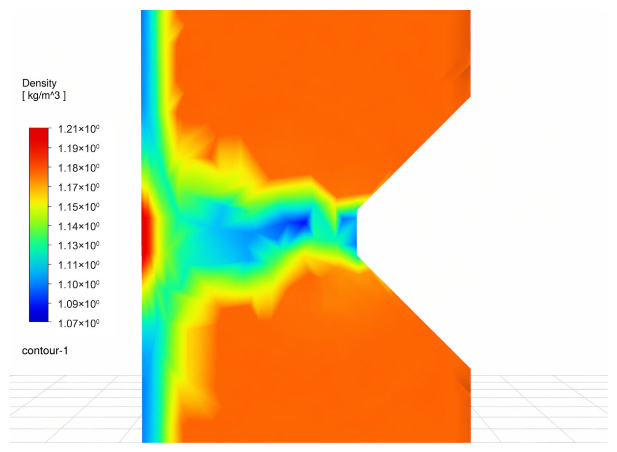
The density contour (Figure 6) provides complementary evidence of compressibility effects within the gas jet. A distinct low-density region is observed in the accelerated jet core and immediately downstream of the slot exit, while the ambient region retains an approximately uniform higher density. The strongest density gradients occur across the jet shear layer and near the impingement zone, consistent with rapid acceleration, and the baseline simulation captures the essential jet impingement topology on the center plane. These flow features underpin the wall loading that is later quantified through the extracted wall static pressure and wall shear stress distribution for coupling with the film thickness model.

4.2. Wall Pressure and Wall Shear Stress Distributions

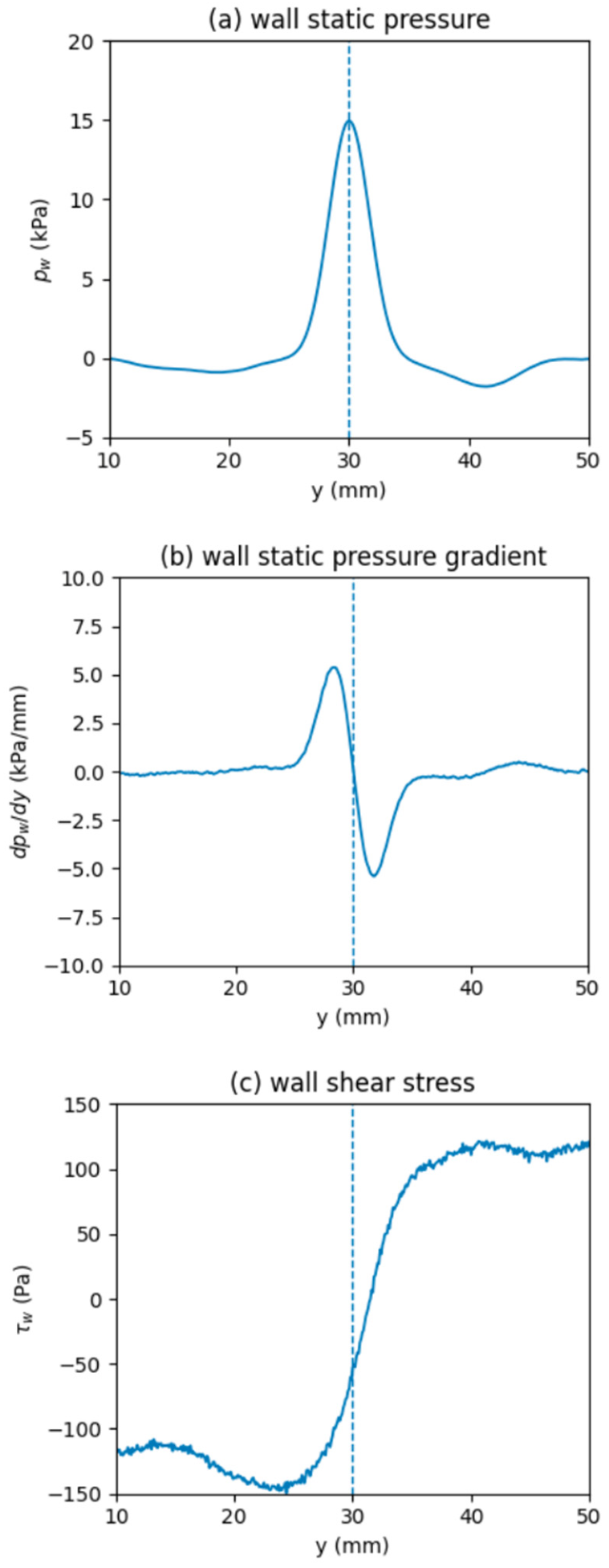
Figure 7 presents the time-averaged wall loading extracted along the strip direction y , with the stagnation point marked at y = y 0 = 30 m m (dashed line). A pronounced wall static pressure peak is observed at the stagnation point, reaching approximately 15 kPa (Figure 7a), which is consistent with the impingement of the air knife jet and the associated momentum turning near the wall. Away from the impingement region, the wall pressure relaxes toward values close to the ambient reference, indicating that the wall-normal jet loading is highly localized around y 0 .
The corresponding wall pressure gradient d p ω / d y exhibits a clear bipolar structure around y 0 (Figure 7b). The gradient attains a positive extremum of about +5 kPa/mm slightly upstream of y 0 , followed by a negative extremum of about −5 kPa/mm downstream. This strong localized gradient provides a key driving input to the lubrication-type film model through the pressure gradient term in the governing cubic thickness relation.
The time-averaged wall shear stress τ ω ( y ) (Figure 7c) shows a marked transition across the stagnation point. Upstream of y 0 , τ ω remains negative with a magnitude on the order of −100 to −140 Pa, while downstream it rapidly increases and becomes positive, approaching a plateau of approximately +110 to +130 Pa. The sign change of τ ω ( y ) across y 0 reflects the reversal of the near-wall flow direction between the upstream and downstream sides of the stagnation region, and it is consistent with the development of a wall jet flow away from the impingement zone. Together, the profiles p ω ( y ) , d p ω d y , and τ ω ( y ) provide physically consistent wall inputs for the coupled film thickness model in Section 4.3, enabling prediction of the coating thickness distribution h ( y ) and the representative final thickness h f i n a l .

4.3. Predicted Coating Thickness and Operating Window

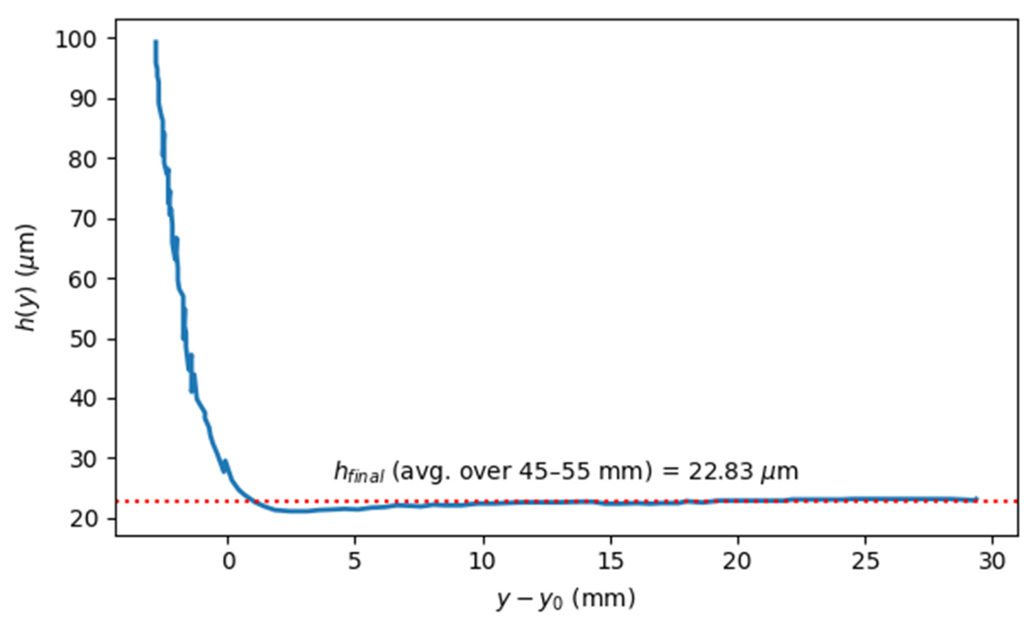
Figure 8 presents the predicted coating thickness distribution h y along the strip direction, plotted against the shifted coordinate y y 0 , where y 0 = 30 mm denotes the stagnation location. The thickness exhibits a rapid decrease in the immediate vicinity of the wiping region (near y y 0 0 ), followed by a gradual relaxation toward a quasi-plateau further downstream. This sharp drop is consistent with the strong localized wall loading extracted from the LES, where the impingement pressure peak and the associated pressure gradient and shear stress extrema provide the dominant driving terms in the lubrication-type film formulation.
Downstream of the impingement zone, the profile becomes nearly invariant with respect to y , indicating that the film reaches a stabilized thickness after the main wiping action. A representative final thickness is therefore defined as the downstream interval average over y   [45, 55] mm, yielding h f i n a l =22.83 μm. This scalar measure is used in the subsequent parametric sweeps to quantify thickness trends and to construct operating window maps as functions of P 0 and H .
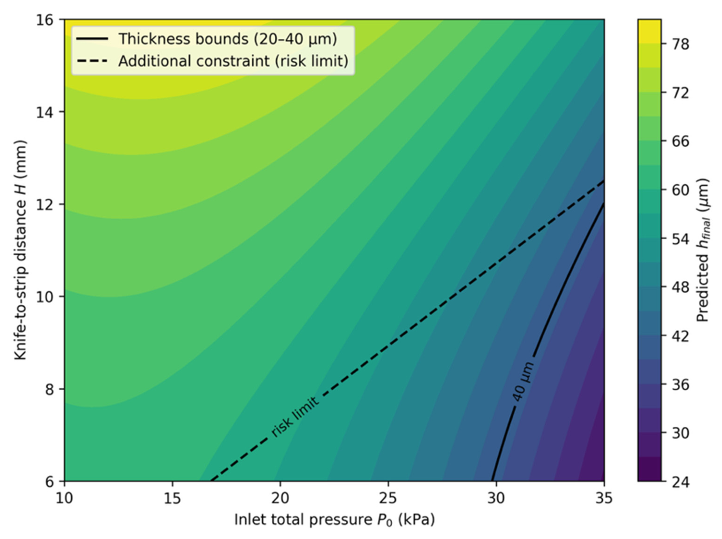
Figure 9 summarizes the operating window map constructed from the coupled LES film model by sweeping the inlet total pressure P 0 and the air-knife-to-strip distance H . The colormap represents the predicted final thickness h f i n a l . A clear monotonic trend is observed: increasing P 0 reduces h f i n a l , whereas increasing H results in a thicker coating, consistent with stronger (weaker) jet impingement and wall loading at higher (lower) jet momentum.
The solid contour lines indicate the predicted thickness bounds defining the target coating range. The dashed line is included as an additional practical risk indicator, rather than a strict mathematical or physical critical boundary. It is used to mark the onset of operating conditions associated with increasingly aggressive wiping, under which the available process margin may become reduced. The operating window can therefore be interpreted by considering both the target thickness range and this additional practical guideline. The map highlights that although very thin coatings can be achieved at high P 0 and small H, such conditions may involve a tradeoff between stronger wiping action and process robustness.

4.4. Validation and Limitations

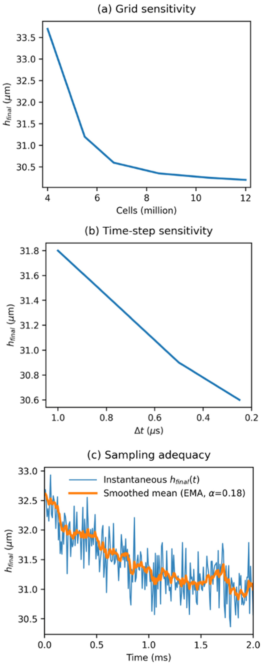
Figure 10 provides numerical adequacy checks for the coupled LES film framework in terms of the predicted final thickness h f i n a l , which is defined consistently with Section 3.2 as the downstream interval average of h y over y   [45, 55] mm. Figure 10a examines grid sensitivity by comparing h f i n a l obtained on a sequence of meshes with increasing total cell count. The curve shows a clear convergence trend: h f i n a l changes rapidly when moving from a coarse grid to an intermediate grid, but the variation becomes progressively smaller as the grid is refined. This behavior indicates that the baseline mesh lies in the asymptotic region where further refinement produces only marginal changes in h f i n a l . Since the film model is driven by time-averaged wall quantities p ω ¯ y and τ ω ¯ y , this check supports that the baseline mesh provides sufficient resolution for extracting wall loading for the coupling analysis.
Figure 10b evaluates the time-step sensitivity by repeating the same baseline operating condition with different fixed time steps Δ t . The baseline time step was initially selected with reference to values commonly used in related LES studies, and its adequacy for the present model was further assessed through this sensitivity check. A monotonic reduction of h f i n a l variation is observed as Δ t decreases, and the curve approaches a plateau at smaller Δ t , indicating diminishing temporal discretization effects. The chosen baseline value t = 5.0 ×   10 7 s is therefore expected to provide an adequate compromise between computational cost and numerical accuracy for the present LES, such that further reduction of t would only lead to a minor change in h f i n a l . This indicates that the selected time step is not arbitrary but lies in a range where temporal discretization effects become small.
Figure 10c addresses sampling adequacy, which is critical for LES because instantaneous quantities exhibit intrinsic unsteadiness. The instantaneous h f i n a l ( t ) shows strong temporal fluctuations, whereas the cumulative mean gradually stabilizes as the sampling time increases. The progressive flattening of the cumulative mean curve indicates that the sampling window T S used for time averaging is sufficiently long to obtain statistically converged driving inputs for the film model, namely p ω ¯ y and τ ω ¯ y , and consequently a stable estimate of h f i n a l . Overall, the three checks shown in Figure 10 demonstrate that the reported trends and operating window boundaries are numerically consistent within the present discretization and sampling choices. Nevertheless, it should be noted that the coating thickness is predicted through a film model driven by LES-extracted wall loading rather than by explicitly resolving free surface dynamics; thus, phenomena such as interface deformation, droplet entrainment or splashing under extreme wiping conditions are not directly captured and may affect quantitative predictions near the limits of the operating envelope.
Although direct experimental thickness data are not available in the present study, the predicted trends are consistent with those reported in the literature on air knife wiping. In particular, the present results show that increasing the inlet total pressure P 0 leads to a reduction in the final coating thickness, whereas increasing the knife-to-strip distance H   leads to a thicker coating. These tendencies are in qualitative agreement with previous experimental and modeling studies, which generally report that stronger jet impingement and wall loading produce more effective wiping and hence a thinner final coating. This comparison further supports that the coupled framework captures the expected physical response to the key operating parameters.

5. Conclusions

This study developed a coupled framework for coating thickness prediction in hot-dip galvanizing by linking a 3D LES of air knife jets with a lubrication-based thin film model. Time-averaged wall pressure and wall shear stress extracted along the strip direction were used as physically consistent driving inputs, leading to a local cubic equation that accounts for both pressure-gradient effects and gravity. The workflow provides a practical route to convert resolved jet wall loading into thickness distributions, a representative final thickness, and operating window maps in P 0 - H space. While the present results demonstrate the feasibility and trends of the coupled approach, future work will focus on strengthening statistical convergence, refining near-wall resolution, and validating predicted thickness against experimental or plant data, as well as extending the framework to multi-slot air knife configurations.

Author Contributions

Conceptualization, H.L. (Hao Liu); methodology, H.L. (Hao Liu), D.Z., H.C., L.S., H.L. (Hongqiang Liu) and X.W.; software, L.Z., M.Z. and D.P.; validation, L.Z., M.Z. and D.P.; formal analysis, H.L. (Hao Liu); investigation, H.L. (Hao Liu), H.C., L.S., H.L. (Hongqiang Liu) and X.W.; data curation, H.L. (Hao Liu), D.Z., H.C., L.S., H.L. (Hongqiang Liu) and X.W.; writing—original draft preparation, H.L. (Hao Liu); writing—review and editing, H.L. (Hao Liu), H.X. and J.H.; visualization, H.L. (Hao Liu); supervision, H.X., J.H., T.Z. and Z.J.; project administration, H.L. (Hao Liu), H.C., L.S., H.L. (Hongqiang Liu) and X.W.; funding acquisition, Z.J. All authors have read and agreed to the published version of the manuscript.

Funding

This work is financially supported by the University of Wollongong and the HBIS Group collaborative project (Grant No. HG2024147), as well as the Australian Research Council (ARC) Industrial Transformation Training Centre (ITTC) for Innovative Composites for the Future of Sustainable Mining Equipment (Grant No. IC220100028).

Institutional Review Board Statement

Not applicable.

Informed Consent Statement

Not applicable.

Data Availability Statement

The data can be made available upon reasonable request.

Acknowledgments

The authors thank the technicians of the China–Serbia “Belt and Road” Joint Laboratory for Green Steel Manufacturing for their assistance in this work.

Conflicts of Interest

Authors Hongwei Cao, Li Sun and Hongqiang Liu were employed by HBIS Materials Technology Research Institute. Author Xi Wu was employed by Changshu Everbright Material Technology Co., Ltd. The remaining authors declare that the research was conducted in the absence of any commercial or financial relationships that could be construed as a potential conflict of interest.

Abbreviations

The following abbreviations are used in this manuscript:
H knife-to-strip distance, mm
p 0 inlet   total   pressure ,   k P a
T 0 inlet   total   temperature ,   K
U s t r i p strip   speed ,   m / s
h ( y ) local   coating   thickness   along   the   strip ,   m   ( or μm)
h f i n a l representative   final   coating   thickness ,   m   ( or μm)
q volumetric   flow   rate   per   unit   width   in   the   film ,   m 2 / s
q o inlet   film   flux   used   to   close   the   film   model ,   m 2 / s
p pressure ,   P a   ( or   K p a )
p ω ( y ) wall   static   pressure   on   the   strip   surface   as   a   function   of   y ,   P a   ( or   K p a )
d p ω d y wall   pressure   gradient   along   the   strip ,   P a / m
t time ,   s
T S sampling   ( time   average )   window   duration ,   s
Δ t CFD   time   step ,   s
g gravitational   acceleration ,   m / s 2
x coordinate   normal   to   strip   surface ,   m
y coordinate   along   strip   motion ,   m
z spanwise   coordinate ,   m
ω air   knife   slot   width ,   m m
τ ω ( y ) wall   shear   stress   on   the   strip   surface   as   a   function   of   y ,   P a
ρ liquid   density ,   k g / m 3
μ dynamic   viscosity   of   the   coating   melt ,   P a · s
u ( y , x ) film   velocity   component   along   y ,     m / s
v y , x film   velocity   component   along   x ,     m / s
y 0 stagnation   point   location   used   as   reference   for   data   extraction ,   m m
y ~ = y     y 0 shift   coordinate   referenced   to   stagnation   point ,   m m
CFDcomputational fluid dynamics
LESlarge eddy simulation
SGSsub-grid scale model
WALEwall adapting local eddy viscosity SGS model
PISOpressure implicit with splitting of operators
VOFvolume of fluid

References

  1. Goodwin, F.E. Overview of Recent Advancements in Hot Dip Metallic Coatings for Steel. Trans. Indian Inst. Met. 2023, 76, 2295–2305. [Google Scholar] [CrossRef]
  2. Soufiani, A.Y.; McDermid, J.R.; Hrymak, A.N.; Goodwin, F.E. Numerical Simulation of Single- and Multiple-Slot Air Knives for Estimation of Final Coating Thickness in the Hot-Dip Galvanizing Process. In Proceedings of the AISTech 2016 Conference Proceedings, Pittsburgh, PA, USA, 16–19 May 2016. [Google Scholar]
  3. Wang, L.-X.; Fang, F.; Li, J.-W. The Effect of Air Knife Wiping Speed on Galvanized Coating Weight and Thickness. In Proceedings of the 2nd Annual International Conference on Advanced Material Engineering (AME 2016), Wuhan, China, 15–17 April 2016. [Google Scholar]
  4. Bao, C.; Kang, Y.; Li, Y. Numerical Simulation of the Effects of Air Knives on Coating Thickness. In Proceedings of the 2016 International Forum on Energy, Environment and Sustainable Development, Shenzhen, China, 16–17 April 2016. [Google Scholar]
  5. Fang, F.; Chen, Y.M.; Li, J.W.; Wang, G. Coating Quality of Hot Dipped Steel with Different Zinc Bath Chemistries and Air Knife Flow Rates. In Proceedings of the Advanced High Strength Steel and Press Hardening, Changsha, China, 15–18 October 2015; pp. 239–244. [Google Scholar]
  6. Zhang, H.; Li, H.; Fu, Y.; Li, L. Simulation Analysis of Different Thickness Control in the Continuous Hot-Dip Galvanizing Process. In Proceedings of the 2015 6th International Conference on Manufacturing Science and Engineering, Qingdao, China, 17–19 July 2015. [Google Scholar]
  7. Gao, P.; Liu, M.; Lin, F.; Liu, C.; He, A.; Li, F.; Xu, L. Research on the Prediction Model of Zinc Coating Thickness of Continuous Hot-Dip Galvanized Strip Steel Based on Gaussian Process Regression. Steel Res. Int. 2025; early view. [CrossRef]
  8. Tamadonfar, P.; Hrymak, A.N.; McDermid, J.R.; Goodwin, F.E. Investigation of Coating Thickness Sensitivity in Air Knife Coating. In Proceedings of the 15th International Coating Science and Technology Symposium, Saint Paul, MN, USA, 13 September 2010. [Google Scholar]
  9. Takeda, G.; Takahashi, H.; Kabeya, K. Jet Flow Characteristics of 3-Slot Nozzle in Gas Wiping Process at Continuous Galvanizing Line. ISIJ Int. 2017, 57, 1087–1093. [Google Scholar] [CrossRef]
  10. Yuan, S.; Zhou, X.; Huang, Y.; Yang, P. Influence of Air Knives on Liquid Zinc Flow in Galvanising Bath. Ironmak. Steelmak. 2016, 43, 83–87. [Google Scholar] [CrossRef]
  11. Yoon, H.G.; Chung, M.K. Development of Novel Air-Knife System to Prevent Check-Mark Stain on Galvanized Strip Surface. ISIJ Int. 2010, 50, 752–759. [Google Scholar] [CrossRef]
  12. So, H.; Yoon, H.G.; Chung, M.K. CFD Analysis of Sag Line Formation on the Zinc-Coated Steel Strip after the Gas-Jet Wiping in the Continuous Hot-Dip Galvanizing Process. ISIJ Int. 2011, 51, 115–123. [Google Scholar] [CrossRef][Green Version]
  13. Hrymak, A.N.; Elsaadawy, E.A.; Hanumanth, G.; McDermid, J.R.; Goodwin, F.E.; Box, P.O. Air Knife Coating Weight Models. Aistech-Conf. Proc. 2005, 2, 393. [Google Scholar]
  14. Lacanette, D.; Gosset, A.; Vincent, S.; Buchlin, J.-M.; Arquis, É. Macroscopic Analysis of Gas-Jet Wiping: Numerical Simulation and Experimental Approach. Phys. Fluids 2006, 18, 042103. [Google Scholar] [CrossRef]
  15. Mendez, M.A.; Gosset, A.; Scheid, B.; Balabane, M. Dynamics of the Jet Wiping Process via Integral Models. J. Fluid Mech. 2021, 911, A47. [Google Scholar] [CrossRef]
  16. Myrillas, K.; Rambaud, P.; Mataigne, J.-M.; Gardin, P.; Vincent, S.; Buchlin, J.-M. Numerical Modeling of Gas-Jet Wiping Process. Chem. Eng. Process. Process Intensif. 2013, 68, 26–31. [Google Scholar] [CrossRef]
  17. Eßl, W.; Pfeiler, C.; Reiss, G.; Ecker, W.; Riener, C.K.; Angeli, G. LES-VOF Simulation and POD Analysis of the Gas-Jet Wiping Process in Continuous Galvanizing Lines. Steel Res. Int. 2018, 89, 1700362. [Google Scholar] [CrossRef]
  18. Hirt, C.W.; Nichols, B.D. Volume of Fluid (VOF) Method for the Dynamics of Free Boundaries. J. Comput. Phys. 1981, 39, 201–225. [Google Scholar] [CrossRef]
  19. Yahyaee Soufiani, A.; McDermid, J.R.; Hrymak, A.N.; Goodwin, F.E. Numerical Investigation of Multiple-Slot Jets in Air-Knife Wiping. J. Coat. Technol. Res. 2017, 14, 1015–1028. [Google Scholar] [CrossRef]
  20. Yuan, Y.; Li, C. Numerical Simulation on the Pressure Field of Gas Knives. Adv. Mater. Res. 2012, 354–355, 664–668. [Google Scholar] [CrossRef]
  21. Nicoud, F.; Ducros, F. Subgrid-Scale Stress Modelling Based on the Square of the Velocity Gradient Tensor. Flow Turbul. Combust. 1999, 62, 183–200. [Google Scholar] [CrossRef]
  22. Issa, R.I. Solution of the Implicitly Discretised Fluid Flow Equations by Operator-Splitting. J. Comput. Phys. 1986, 62, 40–65. [Google Scholar] [CrossRef]
  23. Ritcey, A.; McDermid, J.R.; Ziada, S.; Goodwin, F.E. Measuring Wall Shear Stress Under an Air Knife Model Using Oil Film Interferometry. In Proceedings of the AISTech 2016 Proceedings, Pittsburgh, PA, USA, 16–19 May 2016. [Google Scholar]
  24. Soufiani, A.Y.; McDermid, J.R.; Hrymak, A.N.; Goodwin, F.E. Flow Stabilization and Coating Thickness Reduction through Use of Multi-Slot Air-Knife in Gas Jet Wiping. J. Coat. Technol. Res. 2022, 19, 143–158. [Google Scholar] [CrossRef]
  25. Yahyaee Soufiani, A.; Mcdermid, J.R.; Hrymak, A.N.; Goodwin, F.E. A Parametric Study of a Multi-Slot Air Knife for Coating Thickness Reduction. ISIJ Int. 2020, 60, 1040–1051. [Google Scholar] [CrossRef]
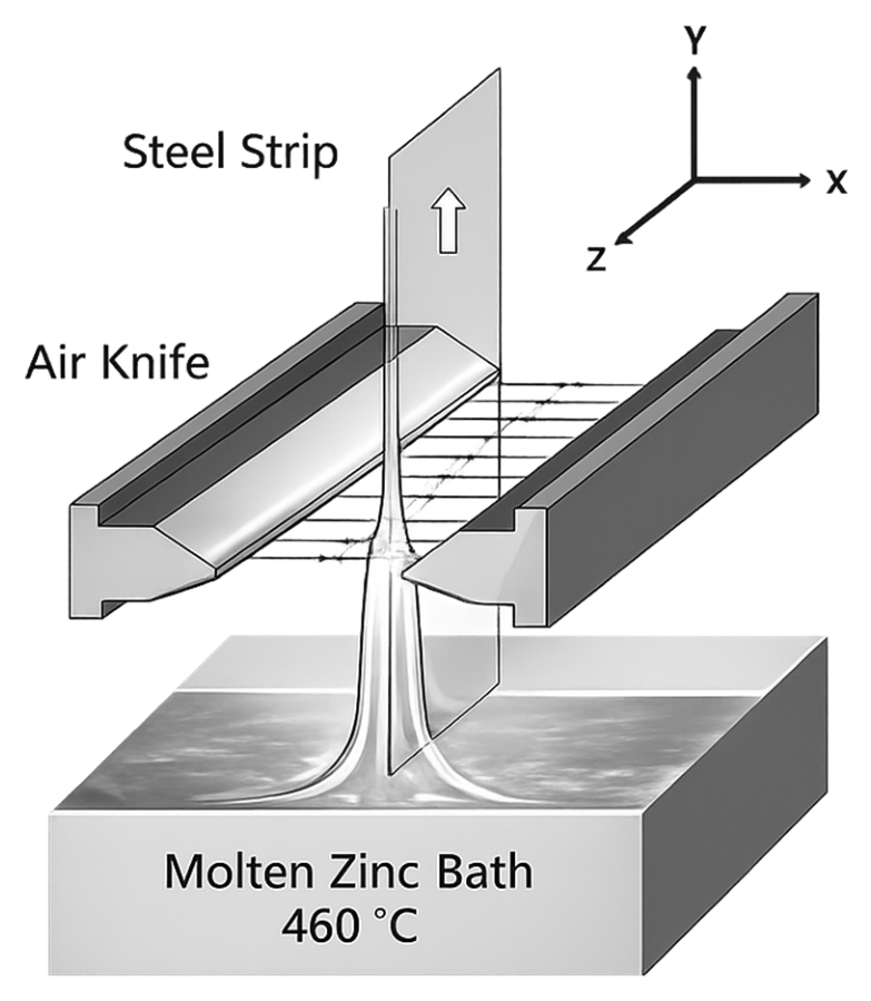
Figure 1. Schematic diagram of the air knife wiping system, the white arrow indicates the moving direction.
Eng 07 00206 g001
Figure 2. Computational geometry, boundary conditions, and wall data extraction location for the air knife wiping simulation. (a) Two-dimensional section view showing the slot width ω , the knife-to-strip distance H , the moving wall steel strip with U s t r i p = 2.5 m / s , the inlet total conditions ( P 0 , T 0 ), and the pressure outlet boundaries ( p = 0 gauge). The stagnation point is located at y = y 0 = 30 m m . (b) Three-dimensional view of the model. The wall line on the strip surface along y is used to extract p ω y and τ ω ( y ) .
Eng 07 00206 g002
Figure 3. Mesh and near-wall resolution for the 3D LES using the WALE sub-grid scale model. (a) Overall review of the computational mesh. (b) Refined mesh in the slot exit and impingement region. (c) Near-wall mesh arrangement adjacent to the moving strip, showing the boundary layer inflation applied for wall pressure and wall shear extraction. The minimum cell size in the refined region is about 0.1 m m .
Eng 07 00206 g003
Figure 4. Workflow of coupling the CFD simulation with the film model using wall pressure and wall shear stress. Solid arrows indicate the main data transfer workflow, whereas dashed arrows indicate auxiliary input, export, and validation links.
Eng 07 00206 g004
Figure 5. Static temperature contour on the center plane ( z = −50 m m ). Static temperature field for the baseline air knife jet impingement case, showing localized gradients near the slot exit, impingement region, and wall jet development along the strip.
Eng 07 00206 g005
Figure 6. Density contour on the center plane ( z = −50 m m ). Density field for the baseline case, highlighting compressibility-induced variations between the high-speed jet core and the ambient region, with the largest gradients occurring across the shear layer surrounding the jet.
Eng 07 00206 g006
Figure 7. Wall static pressure p ω , wall pressure distribution d p ω d y and wall shear stress distribution τ ω ( y ) .
Eng 07 00206 g007
Figure 8. Predicted coating thickness distribution along the strip direction. The thickness profile h y is obtained by solving the film model using LES-extracted time-averaged wall static pressure p ω ¯ y and wall shear stress τ ω ¯ y . The stagnation point is located at y y 0 = 0 m m . A representative final thickness h f i n a l is evaluated in the downstream region where the profile approaches a plateau.
Eng 07 00206 g008
Figure 9. Operating window map.
Eng 07 00206 g009
Figure 10. Validation and adequacy checks.
Eng 07 00206 g010
Disclaimer/Publisher’s Note: The statements, opinions and data contained in all publications are solely those of the individual author(s) and contributor(s) and not of MDPI and/or the editor(s). MDPI and/or the editor(s) disclaim responsibility for any injury to people or property resulting from any ideas, methods, instructions or products referred to in the content.