A Deterministic Calibration Strategy for MOHID-Land Based on Soil Parameter Uncertainty

Abstract

This study investigates the influence of parametric uncertainty in the van Genuchten–Mualem (VGM) model on hydrological simulations and proposes a deterministic, soil-focused calibration strategy within the MOHID-Land model. The approach was applied to the Pedro do Rio watershed to quantify the impact of VGM parameters, typically estimated via pedotransfer functions, on streamflow performance and to reduce uncertainty through targeted calibration. A one-at-a-time sensitivity analysis using the 95% Prediction Uncertainty (95PPU) metric identified the saturated water content (θ_s) and pore-size distribution (n) as the most influential parameters. Calibration scenarios adjusting these parameters, especially Scenario S45 (+30% θ_s, +20% n), significantly improved model performance, increasing the Nash–Sutcliffe Efficiency (NSE) from 0.20 to 0.66 on a daily scale and to 0.80 on a monthly scale during the validation period. Subsequent hydrodynamic refinements raised the daily NSE to 0.72, while monthly performance remained unchanged. The results underscore that soil parameter uncertainty plays a central role in long-term water balance representation, while hydrodynamic parameters primarily influence short-term dynamics in steep, responsive basins. Overall, the proposed strategy provides a computationally efficient alternative to fully automatic calibration methods, delivering robust performance while maintaining physical consistency, particularly in data-scarce environments.

1. Introduction

Understanding soil–water interactions in the unsaturated zone is fundamental for simulating hydrological processes and supporting sustainable water resources management. Soil hydraulic functions, which describe the relationships between soil water pressure head ($h$), volumetric water content ($\theta$), and hydraulic conductivity ($K$), play a central role in modeling water transport within the soil–vegetation–atmosphere continuum [1]. These relationships form the physical basis of process-based hydrological models, such as JULES [2], HYDRUS [3], DSSAT-HYDRUS-1D [4], and SWAP [5]. In these models, soil hydraulic parameterization directly affects the simulation of key hydrological processes, including soil water balance, root water uptake, solute transport, and groundwater recharge [4,6,7], thereby influencing the overall accuracy and reliability of hydrological predictions.

Among the various formulations available to represent soil hydraulic behavior, the van Genuchten–Mualem (VGM) model is one of the most widely adopted analytical frameworks. It combines the soil water retention curve proposed by van Genuchten [8] with the hydraulic conductivity formulation developed by Mualem [9], providing a flexible yet physically grounded description of unsaturated flow. Despite its widespread use, the predictive performance of the VGM model is highly sensitive to the accurate estimation of its parameters, including saturated hydraulic conductivity ($K_{sat}$), residual water content (${\theta }_r$), saturated water content (${\theta }_s$), and the shape parameters $\alpha$ and $n$. Uncertainties associated with these parameters, particularly when derived from pedotransfer functions or sparse soil sampling, can propagate through hydrological models and lead to substantial errors in simulated fluxes and states [10,11].

This issue becomes especially critical in complex, physically based, and spatially distributed hydrological models such as MOHID-Land. MOHID-Land solves the three-dimensional Richards equation using finite volume methods to simulate water flow in variably saturated porous media. In its standard configuration, the model integrates the van Genuchten–Mualem formulation with pedotransfer approaches, such as Rosetta, to estimate hydraulic parameters from basic soil physical properties at the grid-cell level. However, the strong horizontal and vertical heterogeneity of soil properties within catchments, combined with the intrinsic uncertainty of pedotransfer functions and the frequent reliance on interpolated soil data from limited sampling campaigns, results in considerable uncertainty in parameter values at the watershed scale [12]. As emphasized by Liao et al. [11], such uncertainty is often driven by small sample sizes and interpolation artifacts, underscoring the persistent challenge of accurately representing soil hydraulic properties in distributed hydrological modeling.

Given these uncertainties, model calibration plays a fundamental role in aligning simulations with observed hydrological responses. Over the past decades, numerous calibration approaches have been proposed, ranging from deterministic optimization techniques to probabilistic and Bayesian frameworks. For instance, Abbaspour [13] introduced the SUFI-2 algorithm, which integrates sensitivity analysis and uncertainty assessment through iterative sampling, while Telles et al. [14] applied multi-objective automatic calibration strategies to small urban watersheds in Brazil. Although effective in many contexts, such automatic or semi-automatic calibration methods are often computationally demanding. This limitation is particularly pronounced for high-resolution, three-dimensional, physically based models like MOHID-Land, which typically require long simulation periods and substantial computational resources. Consequently, the direct application of these methods to large-scale or long-term simulations remains impractical, highlighting the need for calibration strategies that explicitly account for model complexity and computational constraints.

Several studies have investigated parameter sensitivity and calibration strategies in hydrological models, emphasizing the role of parameter uncertainty and the complex interactions among soil hydraulic properties in controlling model performance [10,11,15,16,17].

Within this context, Oliveira et al. [18] conducted a pioneering study to investigate parameter sensitivity in MOHID-Land. Their study applied a local sensitivity analysis, varying individual parameters independently, and focused exclusively on $K_{sat}$. While this work provided valuable initial insights, it did not address potential interactions among soil hydraulic parameters or explore systematic calibration strategies. Building upon this foundation, Sales et al. [19] conducted a localized sensitivity analysis of all VGM parameters within MOHID-Land. Their results demonstrated that the parameters $n$ and ${\theta }_s$ exerted the strongest influence on model performance, followed by $K_{sat}$, ${\theta }_r$, and $\alpha$. Nevertheless, that analysis was limited to a fixed perturbation of ±10% around reference values, offering only a local perspective on parameter sensitivity. Even within this restricted range, the study showed that simultaneous calibration of all five parameters substantially improved model performance, suggesting the presence of nontrivial interactions among parameters.

To further investigate these interactions, Sales et al. [20] advanced the analysis by implementing a combinatorial calibration strategy that systematically evaluated all possible parameter combinations. Their findings confirmed that joint calibration of the five VGM parameters produced the best overall performance. However, the improvements were not additive, indicating strong nonlinear interactions among parameters. Notably, calibrating only ${\theta }_s$ and $n$ already yielded substantial performance gains, and the inclusion of a third parameter, whether $K_{sat}$, $\alpha$, or ${\theta }_r$, consistently enhanced model accuracy. Although full five-parameter calibration remained optimal, the marginal gains beyond the third parameter were comparatively modest, raising important questions regarding calibration efficiency and parameter prioritization in computationally intensive models.

Despite these advances, a key limitation persists across the existing studies. Both Sales et al. [19] and Sales et al. [20] restricted parameter variation to a narrow range of ±10% around baseline estimates. As a result, the behavior of MOHID-Land under broader, yet physically plausible, ranges of soil hydraulic parameters remain largely unexplored. Moreover, the extent to which parameter uncertainty at larger scales translates into predictive uncertainty, and how this information can be leveraged to design efficient calibration strategies, has not yet been systematically addressed for MOHID-Land. Addressing this gap constitutes the main objective of the present study.

Addressing parameter uncertainty explicitly has become an increasingly important objective in hydrological modeling. A variety of uncertainty estimation techniques have been proposed, ranging from methods that define upper and lower predictive bounds [15] to Bayesian Markov Chain Monte Carlo (MCMC) approaches that sample posterior parameter distributions [16,17]. Among these approaches, the 95% prediction uncertainty (95PPU) framework offers a practical and computationally efficient means of quantifying the effects of parameter uncertainty on model outputs. The 95PPU represents the uncertainty envelope bounded by the 2.5th and 97.5th percentiles of simulated values at each time step and is commonly used to assess the proportion of observed streamflow captured within this envelope, with narrower bands and higher coverage indicating improved model reliability [13].

By integrating this uncertainty-based diagnostic with a structured and deterministic calibration strategy, the present study seeks to bridge sensitivity analysis and uncertainty quantification in a manner that is both computationally feasible and physically meaningful for complex models such as MOHID-Land. In contrast to previous approaches based on local sensitivity analyses or narrow parameter ranges, the proposed framework considers broader physically plausible parameter spaces while maintaining a structured calibration logic. Rather than relying on fully automated optimization, the proposed framework prioritizes parameters that exhibit high influence and constrained uncertainty, while parameters with limited impact or high variability may be fixed or treated separately. This distinction allows the methodology to reduce computational demand while preserving process interpretability. In doing so, the methodology enhances calibration efficiency, improves robustness, and provides deeper insight into the internal parameter dynamics governing hydrological responses in high-complexity, physically based watershed models.

2. Materials and Methods

This section describes the study area, model configuration, and the methodological framework adopted. For clarity, the proposed approach is structured into the following main stages: (i) establishment of a baseline simulation using soil hydraulic parameters derived from pedotransfer functions; (ii) implementing a systematic uncertainty analysis based on one-at-a-time (OAT) perturbations of the van Genuchten–Mualem (VGM) parameters; (iii) identifying the parameters exerting dominant control over model response; (iv) formulating a structured calibration strategy focused on the most influential parameters; (v) assessing calibration performance under different parameter combinations and hydraulic anisotropy conditions; and (vi) validating the selected model configurations using an independent simulation period.

2.1. Study Area

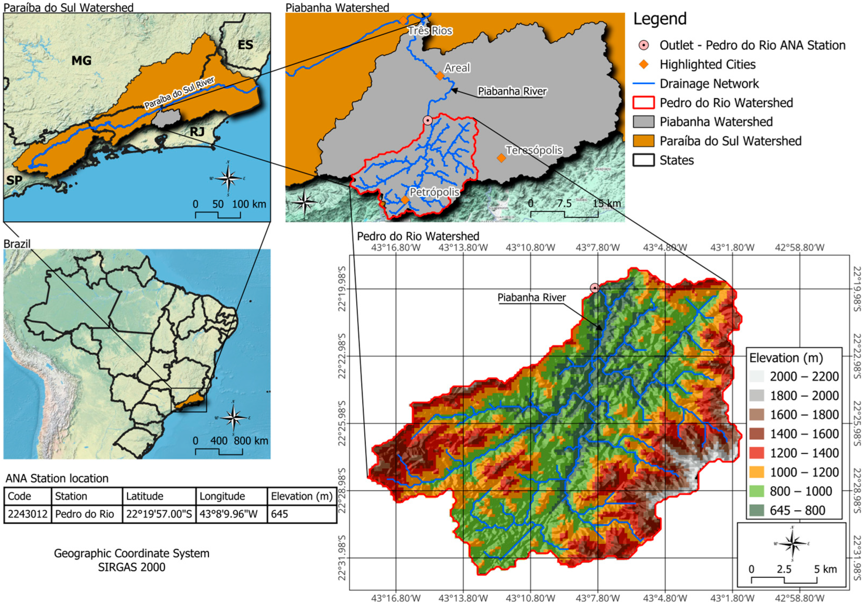
The Pedro do Rio watershed is situated in the mountainous sector of the municipality of Petrópolis, in the state of Rio de Janeiro, southeastern Brazil, and encompasses an area of approximately 420 km², corresponding to nearly 55% of the municipal territory. The basin is embedded within the Serra do Mar mountain range and lies entirely within the Atlantic Forest biome, a globally recognized biodiversity hotspot characterized by high levels of endemism and strong ecological relevance. From a hydrological standpoint, the watershed is part of the Piabanha River system, which constitutes one of the main tributaries of the Paraíba do Sul River basin, a strategic freshwater system that supports domestic supply, agriculture, and industrial activities across the states of São Paulo, Minas Gerais, and Rio de Janeiro (Figure 1).

Owing to its environmental representativeness and hydrological relevance, the Pedro do Rio watershed was selected as one of the pilot basins within the Integrated Studies in Experimental and Representative Basins program (EIBEX), a national initiative coordinated by the Brazilian Geological Survey (SGB/CPRM). The EIBEX program is designed to establish long-term monitoring in watersheds that typify the diverse physical, environmental, socioeconomic, and water-resource dynamics observed across Brazil [21]. In this context, the Pedro do Rio basin serves as a reference site for hydrological research, model development, and methodological testing. Its outlet is instrumented with a streamflow gauging station operated by the National Water and Sanitation Agency (Agência Nacional de Águas e Saneamento Básico—ANA), providing continuous and reliable discharge observations that are essential for model calibration and validation.

In addition to its strategic role within national monitoring programs, the watershed is characterized by a high degree of physiographic complexity, which poses significant challenges for hydrological modeling. Previous studies have highlighted the difficulty of accurately representing unsaturated zone processes and lateral subsurface flow in this region, particularly during low-flow periods, due to the combined effects of steep terrain, heterogeneous soils, and strong climatic gradients [22,23]. These characteristics make the Pedro do Rio watershed especially suitable for testing physically based and distributed hydrological models under demanding conditions.

The watershed is influenced by the urban dynamics of Petrópolis, which exert increasing pressure on water resources through enhanced water demand and land-use transformation processes. Agricultural activities also play an important role in the region, particularly in the production of cereals, legumes, and oilseeds. While economically relevant, these activities intensify water withdrawals and contribute to soil erosion, sediment yield, and nonpoint-source pollution associated with agrochemical runoff, thereby affecting both water quantity and quality.

The basin exhibits pronounced topographic variability, with elevations ranging from approximately 645 m at the outlet to nearly 2200 m in the headwater regions, resulting in a total relief of approximately 1450 m. Steep slopes dominate the landscape: 44.6% of the watershed area is classified as strongly undulating terrain (20–35%), while an additional 36.4% is characterized as mountainous relief (45–75%). This rugged morphology, combined with unregulated occupation of steep slopes, leads to a heightened susceptibility to landslides and mass movement processes, which directly influence runoff generation, sediment transport, and channel dynamics.

Climatic conditions within the watershed are strongly controlled by elevation. Annual precipitation exceeds 2000 mm in the upper portions of the basin, while lower-elevation areas receive approximately 1300 mm per year. This spatial gradient reflects the orographic effect of the Serra do Mar range, with rainfall generally decreasing from the headwaters toward the outlet. Seasonal variability is pronounced, with the highest rainfall intensities occurring during the austral summer, when convective storms frequently trigger flash floods, soil erosion, and slope instability. The spatial distribution of precipitation and isohyet patterns for the region is detailed in Costa et al. [24].

Land use and land cover within the Pedro do Rio watershed form a heterogeneous mosaic shaped by both natural and anthropogenic processes. Dense Atlantic Forest vegetation covers approximately 62% of the basin, including extensive protected areas within the Serra dos Órgãos National Park, highlighting the ecological and hydrological significance of the region. Agricultural and pastoral lands account for roughly 26% of the watershed and are primarily located along riparian corridors and hillslopes, where they influence infiltration capacity, surface runoff generation, and sediment yield. Urbanized areas currently occupy about 7% of the basin and have expanded in recent decades due to the proximity to the metropolitan region of Rio de Janeiro, increasing impervious surface cover and intensifying hydrological responses such as peak flow amplification, flooding, and slope instability. The remaining portion of the watershed consists mainly of rocky outcrops on steep slopes, which further complicate hydrological processes and limit soil development.

The soil information used in this study originates from the Rio de Janeiro Project, a comprehensive set of multidisciplinary surveys conducted by the Brazilian Geological Survey in collaboration with partner institutions. The resulting soil map covers the entire state of Rio de Janeiro at a scale of 1:250,000 [25] and follows the Brazilian Soil Classification System (SiBCS), developed by EMBRAPA [26]. This classification framework organizes soils according to their pedogenetic evolution, mineralogical composition, and physical and chemical properties.

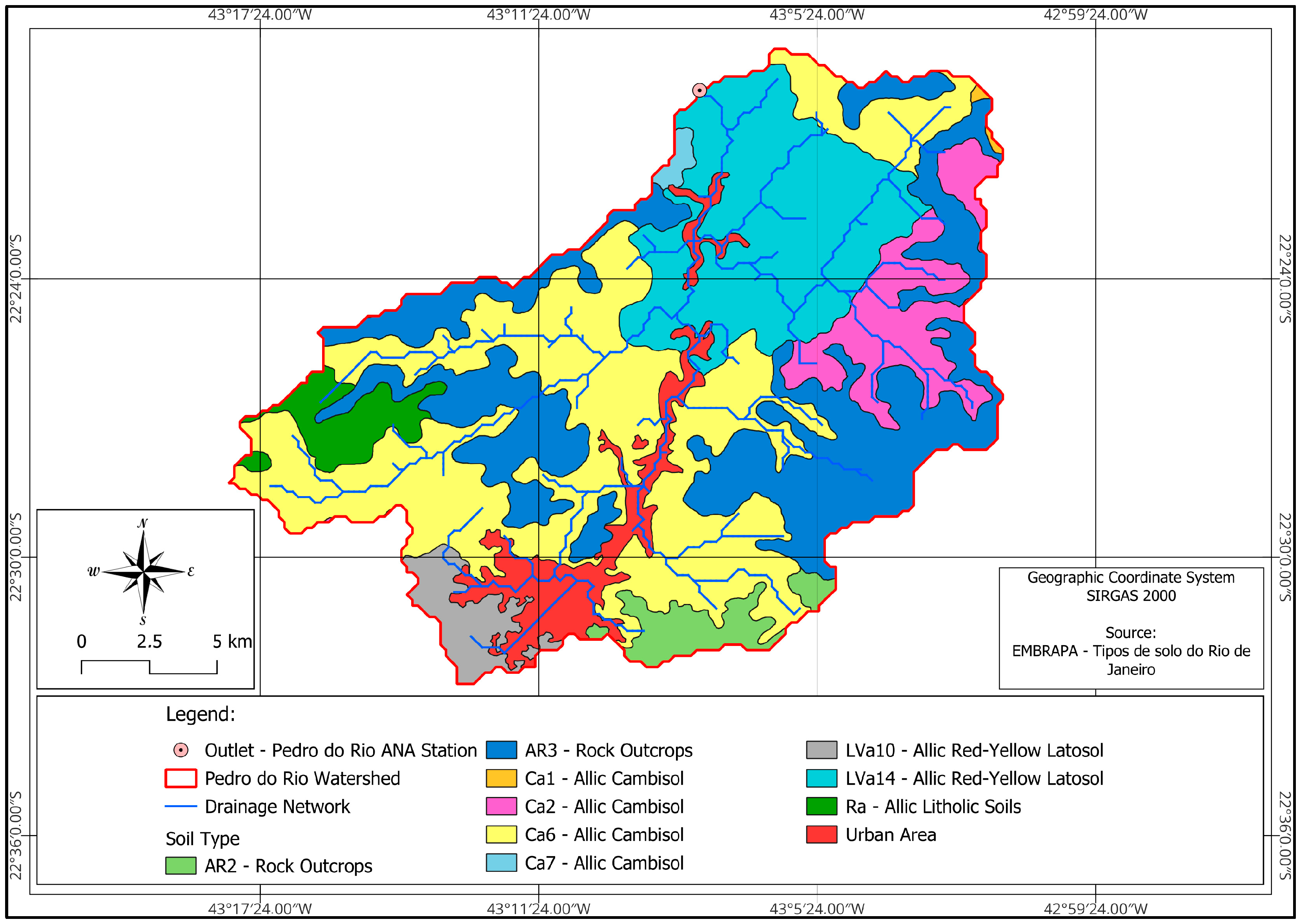
Within the Pedro do Rio watershed, Allic Cambisols constitute the dominant soil class, covering approximately 66.74% of the basin area (Figure 2). These soils are characterized by an intermediate degree of weathering, retention of parent material features, and generally low permeability, with profiles ranging from shallow to moderately deep. The Allic qualifier denotes high aluminum saturation, which is associated with acidic conditions and potential aluminum toxicity, limiting agricultural productivity without corrective management. Several mapped units of this soil class are identified within the basin, including Ca1, Ca2, Ca6, and Ca7, reflecting variations in depth, texture, drainage, and topographic position.

The second-most prevalent soil class is the Allic Red–Yellow Latosol, which occupies approximately 22.83% of the watershed. Latosols are highly weathered, typically very deep soils with relatively homogeneous profiles, high porosity, and favorable drainage conditions, promoting water infiltration and root development. As with Cambisols, this class is subdivided into multiple mapped units, such as LVa10 and LVa14, to capture spatial variability in soil properties. Additional soil units include Allic Litholic Soils, which are shallow and strongly influenced by bedrock, as well as exposed rock outcrops where soil cover is absent. Urban areas are also delineated in the soil map, representing anthropogenic land cover rather than natural soil classes. In total, ten distinct soil classes are identified within the watershed.

Taken together, the combination of complex topography, strong climatic gradients, heterogeneous land use, diverse soil classes, and intense anthropogenic pressure characterizes the Pedro do Rio watershed as a hydrologically intricate and environmentally sensitive system. These characteristics reinforce the need for detailed monitoring and the application of robust, physically based modeling approaches, making the basin a highly suitable case study for investigating soil–water processes and calibration strategies in distributed hydrological models.

2.2. MOHID-Land Model Overview

MOHID-Land is a physically based hydrological model that simulates surface and subsurface processes within a distributed framework. In this study, the description focuses on components directly related to the calibration strategy, particularly soil hydraulic processes and flow routing.

The model is based on the Finite Volume Method (FVM), ensuring mass conservation within each computational cell. The spatial domain is discretized using a structured grid and a layered vertical representation, allowing the simulation of hydrological processes while maintaining numerical stability [27].

Surface and channel flow routing are governed by the Saint-Venant equations, which are particularly relevant in this study due to the hydrodynamic refinement step (Equations (1) and (2)). These equations describe the conservation of mass and momentum under transient conditions. Energy losses due to friction are quantified using Manning’s equation (Equation (3)), ensuring a physically consistent representation of resistance effects across both surface and channelized flow domains [18,20].

$${\displaystyle \frac{\partial A}{\partial t}}+{\displaystyle \frac{\partial Q}{\partial x_i}}=q_L$$

(1)

$${\displaystyle \frac{\partial Q_i}{\partial t}}+v_j{\displaystyle \frac{\partial Q_i}{\partial x_j}}=-g A\left({\displaystyle \frac{\partial H}{\partial x_i}}+S_{fi}\right)$$

(2)

$$S_f={\displaystyle \frac{n_{*}^{2}Q\left|Q\right|}{A^2{R_h}^{4/3}}}$$

(3)

where $Q$ is discharge [m³/s], $A$ is flow area [m²], v is velocity [m/s], $q_L$ is lateral inflow [m³/s/m], $x_i$ is the flow direction, $x_j$ are spatial directions, $g$ is gravitational acceleration [m/s²], $H$ is hydraulic head [m], $S_{fi}$ is the friction slope [m/m], $n_{*}$ is Manning’s roughness coefficient [s/m^1/3], $R_h={\displaystyle \frac{A}{P}}$ is the hydraulic radius [m], and $P$ is the wetted perimeter [m]. The term $Q\left|Q\right|$ ensures friction acts in the direction opposite to the flow.

Vegetation dynamics are represented using a modified version of the EPIC model [28], in which plant growth and root water uptake are simulated based on soil moisture conditions and stress response functions [29]. Although included in the model structure, vegetation processes were not a primary focus of the calibration strategy.

Atmospheric forcing includes precipitation, air temperature, solar radiation, relative humidity, and wind speed, with evapotranspiration estimated using the dual crop coefficient approach [30].

2.2.1. MOHID-Land Soil Water Dynamics and Porous Media Representation

Soil water flow in MOHID-Land is governed by the Richards equation (Equation (4)), which describes transient water movement in variably saturated porous media as a function of hydraulic gradients and soil hydraulic properties [31].

$${\displaystyle \frac{\partial \theta }{\partial t}}=-{\displaystyle \frac{\partial Q_i}{x_d}}-S\left(h\right)={\displaystyle \frac{\partial }{x_d}}\left(K\left(\theta \right){\displaystyle \frac{\partial H}{\partial x_d}}\right)A-S\left(h\right)$$

(4)

where $K\left(\theta \right)$ is the unsaturated hydraulic conductivity [m/s], $Q$ is the flux [m³/s], $A$ is the area [m²], $\theta$ is the water content [m³/m³], $H$ is the hydraulic gradient (topography + hydrostatic pressure + suction pressure) [m], $x_d$ is the flow direction, and $S\left(h\right)$ is the term for water uptake from the soil by plant roots [m³/s].

This equation is solved within a three-dimensional soil domain that explicitly represents both vertical percolation and lateral subsurface flow, allowing continuous redistribution of soil moisture under saturated and unsaturated conditions. In contrast to conceptual or semi-distributed models, such as SWAT, which activate percolation and lateral flow only after soil layers exceed saturation thresholds [27,32], MOHID-Land resolves internal fluxes directly within the porous medium as a dynamic response to pressure gradients.

The governing formulation results from coupling the Buckingham–Darcy flux law with the continuity equation, such that hydraulic conductivity reaches its maximum value under saturated conditions and decreases nonlinearly as soil moisture declines [31]. This structure provides a physically consistent representation of infiltration, drainage, and internal redistribution processes within the soil profile.

Spatial variability in hydraulic behavior is represented using a structured grid consistent with the continuum assumption and the concept of a representative elementary volume [33], allowing heterogeneity in soil properties to be incorporated while preserving numerical stability across complex terrain.

Boundary conditions define the interaction between the soil and adjacent compartments. At the lower boundary, an impermeable bedrock layer redirects percolating water laterally along terrain gradients, contributing to subsurface flow and streamflow generation. At the upper boundary, the soil–atmosphere interface applies precipitation, evapotranspiration, and vegetation water uptake as fluxes, with constant atmospheric air pressure imposed.

Soil hydraulic properties are parameterized using the VGM framework (Equations (5) and (6)), which defines both the soil water retention curve and the unsaturated hydraulic conductivity function through nonlinear relationships between matric potential, effective saturation, and conductivity [8,9]. Directional differences in permeability are incorporated through an anisotropy factor ($KF$), defined as the ratio between horizontal and vertical saturated hydraulic conductivity (Equation (7)), where unity denotes isotropic conditions and deviations represent preferential flow directions [34].

$$\theta \left(h\right)={\theta }_r+{\displaystyle \frac{{\theta }_s-{\theta }_r}{{\left[{1+\left(\alpha \left|h\right|\right)}^n\right]}^m}}$$

(5)

$$K\left(\theta \right)=K_{sat} S_e^L{(1-{(1-S_e^{1/m})}^m)}^2$$

(6)

$$KF={\displaystyle \raisebox{1ex}{$K_{sat,hor}$}\!\left/ \!\raisebox{-1ex}{$K_{sat}$}\right.}$$

(7)

where ${\theta }_s$ is the saturated water content [m³/m³], ${\theta }_r$ is the residual water content [m³/m³], $h$ is the suction pressure [m], $K_{sat}$ is the saturated hydraulic conductivity [m/s], $\alpha$ is the curve adjustment parameter, related to the inverse of the air entry [m⁻¹], $n$ is the curve adjustment parameter, related to the pore-size distribution [dimensionless], $m$ is obtained from the relation $1-1/n$, $S_e$ is the effective saturation [dimensionless], $L$ is the empirical pore connectivity [m], equal to 0.5 [8], $KF$ is the hydraulic conductivity multiplying factor [dimensionless], and $K_{sat,hor}$ is the horizontal saturated conductivity [m/s].

Together, these formulations establish the physical basis for the calibration strategy adopted in this study, particularly with respect to soil hydraulic parameter adjustment and hydrodynamic refinement.

2.2.2. Model Set-Up (Baseline Simulations—S1)

The MOHID-Land model was implemented over the Pedro do Rio watershed using a regular horizontal grid with a spatial resolution of 0.002° (approximately 200 m), comprising 160 rows and 200 columns. This resolution represents a compromise between spatial detail and computational cost, being sufficient to resolve topographic variability and drainage patterns at the watershed scale while maintaining computational efficiency.

The lower-left corner of the grid is anchored at geographic coordinates 43.36° W and 22.59° S. Computational processes were restricted to the watershed boundaries, with grid cells outside the basin excluded from simulations. Topographic information was obtained from the Topodata Digital Elevation Model (DEM) with a native spatial resolution of 30 m [35] and interpolated to the model grid.

The river network was represented explicitly within the model domain. Channel geometry was parameterized using trapezoidal cross-sections derived from in situ field surveys conducted between 2019 and 2021 under the coordination of the Piabanha Watershed Committee. Cross-section dimensions were defined as a function of upstream drainage area, with measured sections assigned to control nodes along the drainage network. For intermediate nodes without direct measurements, cross-section parameters were linearly interpolated between adjacent control points, ensuring spatial continuity along the channel network (

Table 1. Dimensions of cross-sections based on field measurements.

Drainage Area (km2)	Heights (m)	Top Width (m)	Bottom Width (m)
2.00	1.50	3.00	1.00
6.32	2.00	4.60	1.00
12.60	2.00	5.10	2.00
34.40	2.00	8.70	2.00
49.18	5.00	11.20	6.00
103.45	5.00	14.00	6.00
419.33	5.00	19.00	6.00

Note: Adapted from Sales et al. [17].

).

Land use and land cover information was obtained from the MapBiomas Project [36] at a spatial resolution of 30 m. Based on these data, land cover was grouped into three dominant classes, forest, pasture, and agriculture, supplemented by urban areas and rocky outcrops where applicable. Each class was assigned Manning’s roughness coefficients ranging from 0.03 to 0.16 s·m^−1/3, following Chow [37]. Crop coefficients ($K_c$) were specified for different vegetation types and phenological stages according to Allen et al. [30], while Feddes root water uptake parameters were defined based on HYDRUS-1D [38] for pasture and agriculture and Grinevskii [39] for forested areas (

Table 2. Surface and vegetation coefficients.

Land Use Classes	Manning Coefficient	${\mathit{K}}_{\mathit{c}}$			Feddes Coefficients
		Initial	Mid-Season	End Season	${\mathit{h}}_1$	${\mathit{h}}_2$	${\mathit{h}}_3$	${\mathit{h}}_4$
Dense Forest	0.160	0.95	1.00	1.00	0	−1	−3.3	−150
Pasture	0.038	0.40	1.05	0.85	−0.1	−0.25	−8	−80
Agriculture	0.045	0.60	1.15	0.90	−0.1	−0.25	−15	−80
Urban	0.040	-	-	-	-	-	-	-
Rocky Outcrop	0.030	-	-	-	-	-	-	-

). Channel Manning’s roughness was assumed spatially uniform and set to 0.035, following Sales et al. [27].

The subsurface domain was explicitly represented as a three-dimensional system through vertical discretization into seven computational layers, with a nominal maximum depth of 7 m. This depth was selected to adequately represent the active hydrological zone controlling infiltration, storage, and subsurface flow processes, while assuming limited hydraulic interaction with deeper layers due to the presence of underlying bedrock. Importantly, this depth does not correspond to a uniform soil thickness across the domain. Instead, the effective thickness of the soil profile varies spatially as a function of local terrain slope, such that soil layers become progressively thinner in steep hillslope areas and thicker in flatter or valley-bottom regions. This approach enhances the physical realism of the model by accounting for the natural reduction in soil depth on steep slopes, where soil development is limited by erosion and mass wasting processes, while allowing deeper profiles in depositional environments, consistent with observed hillslope–valley soil formation patterns.

The vertical discretization follows the six soil horizons defined by the EMBRAPA soil database, with the two deepest computational layers sharing the hydraulic properties of the 100–200 cm horizon (

Table 3. Vertical discretization of the 3D soil domain.

Model Layers		EMBRAPA Layers
ID	Thickness
1	5 cm	0–5 cm
2	10 cm	5–15 cm
3	15 cm	15–30 cm
4	30 cm	30–60 cm
5	40 cm	60–100 cm
6	300 cm	100–200 cm
7	300 cm

Note: Adapted from Sales et al. [20].

). Soil physical properties, including sand, silt, and clay fractions and bulk density, were obtained from nationwide EMBRAPA datasets [40,41], provided as raster layers at 90 m resolution. To improve spatial consistency, a high-resolution shapefile of soil types specific to the state of Rio de Janeiro was also incorporated. This discretization ensures consistency with the available soil database while preserving the vertical variability required to represent soil water processes.

Soil hydraulic parameters were derived from the EMBRAPA datasets through the Rosetta pedotransfer model, using a fully automated and reproducible workflow implemented via the MOHID Soil Tool (MST). This tool, specifically developed to support MOHID-Land applications, systematically processes soil texture fractions and bulk density for each mapped soil unit and depth interval, ensuring consistency between soil databases and model parameterization [12]. The executable version of the software, along with its user manual is available at: https://github.com/dhiegosales/MOHID-SOIL-TOOL (accessed on 12 December 2025). Additionally, the complete set of input files can be accessed at: https://zenodo.org/records/14914611 (accessed on 23 January 2026).

Through this procedure, the van Genuchten–Mualem hydraulic parameters (${\theta }_r$, ${\theta }_s$, $\alpha$, $n$, $K_{sat}$) were calculated for each soil type and effective depth layer. In total, 60 parameter sets (corresponding to 10 soil types across 6 effective layers) were generated and implemented in MOHID-Land, preserving both vertical and spatial heterogeneity in soil hydraulic properties in accordance with the underlying EMBRAPA soil database. The complete set of hydraulic parameters is provided in Appendix A (

Table A1. Soil properties (EMBRAPA) and corresponding hydraulic parameters generated by the Rosetta pedotransfer model for each soil type and layer—generated in MOHID Soil Tool.

Layer	Soil Type (Polygons)	EMBRAPA INPUT				ROSETTA OUTPUT
		Sand (%)	Silt (%)	Clay (%)	Density (g/cm3)	${\mathit{\theta }}_{\mathit{r}}$ (m3/m3)	${\mathit{\theta }}_{\mathit{s}}$ (m3/m3)	$\mathit{n}$ (-)	$\mathit{\alpha }$(m−1)	${\mathit{K}}_{\mathit{s}\mathit{a}\mathit{t}}$ (m/s)
0–5 cm	AR2—Rock outcrops	51.82	19.34	28.84	1.08	0.106	0.512	1.364	1.033	8.407 × 10−6
0–5 cm	AR3—Rock outcrops	51.02	18.47	30.5	1.06	0.109	0.521	1.356	1.042	8.805 × 10−6
0–5 cm	Ca1—Allic Cambisol	53.1	17.19	29.71	1.07	0.108	0.518	1.357	1.088	8.930 × 10−6
0–5 cm	Ca2—Allic Cambisol	50.18	16.9	32.92	1.11	0.111	0.514	1.344	1.094	7.218 × 10−6
0–5 cm	Ca6—Allic Cambisol	48.37	17.2	34.43	1.15	0.112	0.506	1.338	1.092	5.989 × 10−6
0–5 cm	Ca7—Allic Cambisol	46.27	16.9	36.83	1.13	0.116	0.516	1.330	1.086	6.199 × 10−6
0–5 cm	LVa10—Allic Red–Yellow Latosol	46.37	18.12	35.52	1.18	0.113	0.500	1.334	1.072	5.102 × 10−6
0–5 cm	LVa14—Allic Red–Yellow Latosol	46.9	16.36	36.74	1.18	0.115	0.503	1.328	1.116	5.209 × 10−6
0–5 cm	Ra—Allic Litholic Soils	52.79	18.22	29	1.07	0.107	0.516	1.362	1.061	8.894 × 10−6
0–5 cm	Urban area	45.89	18.8	35.31	1.19	0.113	0.496	1.335	1.057	4.841 × 10−6
5–15 cm	AR2—Rock outcrops	50.58	20.44	28.98	1.04	0.107	0.522	1.365	0.985	9.429 × 10−6
5–15 cm	AR3—Rock outcrops	49.53	19.61	30.86	1.04	0.110	0.526	1.356	1.001	9.163 × 10−6
5–15 cm	Ca1—Allic Cambisol	51.96	19.3	28.74	1.05	0.107	0.520	1.364	1.023	9.372 × 10−6
5–15 cm	Ca2—Allic Cambisol	49.08	17.86	33.06	1.08	0.112	0.521	1.345	1.055	7.841 × 10−6
5–15 cm	Ca6—Allic Cambisol	47.49	18.07	34.43	1.12	0.113	0.513	1.340	1.058	6.563 × 10−6
5–15 cm	Ca7—Allic Cambisol	48.37	17.17	34.46	1.12	0.113	0.514	1.339	1.083	6.690 × 10−6
5–15 cm	LVa10—Allic Red–Yellow Latosol	45.12	19.11	35.77	1.16	0.114	0.505	1.336	1.039	5.365 × 10−6
5–15 cm	LVa14—Allic Red–Yellow Latosol	48.01	16.12	35.87	1.17	0.114	0.504	1.331	1.123	5.539 × 10−6
5–15 cm	Ra—Allic Litholic Soils	50.96	19.39	29.66	1.04	0.108	0.524	1.360	1.012	9.458 × 10−6
5–15 cm	Urban area	45.34	19.03	35.63	1.17	0.113	0.502	1.336	1.044	5.180 × 10−6
15–30 cm	AR2—Rock outcrops	49.56	17.8	32.64	1.09	0.111	0.518	1.347	1.062	7.644 × 10−6
15–30 cm	AR3—Rock outcrops	48.57	16.71	34.72	1.09	0.114	0.522	1.338	1.085	7.487 × 10−6
15–30 cm	Ca1—Allic Cambisol	52.48	15.66	31.86	1.07	0.111	0.523	1.347	1.121	8.736 × 10−6
15–30 cm	Ca2—Allic Cambisol	49.25	15.04	35.71	1.12	0.115	0.517	1.332	1.138	6.840 × 10−6
15–30 cm	Ca6—Allic Cambisol	47.33	15.81	36.86	1.16	0.115	0.509	1.328	1.124	5.679 × 10−6
15–30 cm	Ca7—Allic Cambisol	46.09	15.24	38.67	1.17	0.117	0.509	1.320	1.136	5.360 × 10−6
15–30 cm	LVa10—Allic Red–Yellow Latosol	44.28	17.04	38.68	1.19	0.117	0.503	1.322	1.094	4.756 × 10−6
15–30 cm	LVa14—Allic Red–Yellow Latosol	47.62	14.66	37.72	1.2	0.116	0.501	1.322	1.165	4.949 × 10−6
15–30 cm	Ra—Allic Litholic Soils	50.52	16.43	33.06	1.08	0.112	0.522	1.343	1.096	8.075 × 10−6
15–30 cm	Urban area	45.53	17.1	37.37	1.2	0.115	0.498	1.326	1.099	4.674 × 10−6
30–60 cm	AR2—Rock outcrops	46.36	19.1	34.54	1.15	0.113	0.505	1.340	1.040	5.708 × 10−6
30–60 cm	AR3—Rock outcrops	46.36	17.9	35.74	1.16	0.114	0.505	1.334	1.071	5.520 × 10−6
30–60 cm	Ca1—Allic Cambisol	51.05	17.73	31.23	1.15	0.108	0.500	1.351	1.093	6.378 × 10−6
30–60 cm	Ca2—Allic Cambisol	45.8	16.59	37.61	1.18	0.116	0.504	1.325	1.106	5.094 × 10−6
30–60 cm	Ca6—Allic Cambisol	43.76	15.85	40.39	1.21	0.118	0.502	1.314	1.125	4.395 × 10−6
30–60 cm	Ca7—Allic Cambisol	43.52	15.35	41.13	1.22	0.119	0.501	1.310	1.138	4.224 × 10−6
30–60 cm	LVa10—Allic Red–Yellow Latosol	40.53	16.02	43.45	1.21	0.122	0.507	1.305	1.112	4.170 × 10−6
30–60 cm	LVa14—Allic Red–Yellow Latosol	43	14.09	42.91	1.25	0.121	0.497	1.301	1.171	3.756 × 10−6
30–60 cm	Ra—Allic Litholic Soils	47.52	17.76	34.72	1.15	0.113	0.506	1.338	1.075	5.871 × 10−6
30–60 cm	Urban area	40.26	15.9	43.84	1.23	0.122	0.502	1.302	1.118	3.836 × 10−6
60–100 cm	AR2—Rock outcrops	55.45	16.01	28.53	1.25	0.102	0.472	1.359	1.211	5.097 × 10−6
60–100 cm	AR3—Rock outcrops	55.25	15.24	29.51	1.26	0.104	0.471	1.353	1.230	4.877 × 10−6
60–100 cm	Ca1—Allic Cambisol	59.44	15.43	25.13	1.25	0.097	0.466	1.379	1.272	5.973 × 10−6
60–100 cm	Ca2—Allic Cambisol	55.29	13.92	30.79	1.26	0.105	0.475	1.346	1.259	4.898 × 10−6
60–100 cm	Ca6—Allic Cambisol	51.07	13.16	35.77	1.26	0.112	0.483	1.324	1.240	4.328 × 10−6
60–100 cm	Ca7—Allic Cambisol	50.91	11.99	37.1	1.25	0.114	0.489	1.319	1.262	4.511 × 10−6
60–100 cm	LVa10—Allic Red–Yellow Latosol	44.7	13.56	41.74	1.23	0.120	0.500	1.306	1.185	4.205 × 10−6
60–100 cm	LVa14—Allic Red–Yellow Latosol	48.77	12.54	38.69	1.27	0.116	0.486	1.312	1.241	3.953 × 10−6
60–100 cm	Ra—Allic Litholic Soils	56.81	15.55	27.64	1.25	0.101	0.470	1.364	1.237	5.363 × 10−6
60–100 cm	Urban area	45.44	14.08	40.48	1.25	0.118	0.493	1.309	1.182	3.927 × 10−6
100–200 cm	AR2—Rock outcrops	48.54	13.81	37.65	1.25	0.115	0.488	1.318	1.204	4.201 × 10−6
100–200 cm	AR3—Rock outcrops	49.81	12.53	37.66	1.25	0.115	0.489	1.317	1.242	4.372 × 10−6
100–200 cm	Ca1—Allic Cambisol	52.47	12.71	34.82	1.24	0.111	0.487	1.329	1.254	4.858 × 10−6
100–200 cm	Ca2—Allic Cambisol	52.38	11.66	35.97	1.25	0.113	0.487	1.323	1.281	4.698 × 10−6
100–200 cm	Ca6—Allic Cambisol	48.93	12.36	38.72	1.25	0.116	0.491	1.313	1.240	4.287 × 10−6
100–200 cm	Ca7—Allic Cambisol	49.45	10.98	39.57	1.25	0.117	0.493	1.309	1.275	4.385 × 10−6
100–200 cm	LVa10—Allic Red–Yellow Latosol	45.55	13.22	41.23	1.24	0.119	0.497	1.306	1.199	4.122 × 10−6
100–200 cm	LVa14—Allic Red–Yellow Latosol	50.4	11.49	38.11	1.27	0.115	0.486	1.313	1.276	4.149 × 10−6
100–200 cm	Ra—Allic Litholic Soils	50.51	12.57	36.92	1.24	0.114	0.491	1.320	1.243	4.616 × 10−6
100–200 cm	Urban area	47.28	12.84	39.88	1.26	0.117	0.490	1.309	1.222	3.964 × 10−6

), enabling full transparency and reproducibility of the parameterization process.

Hydraulic conductivity anisotropy was represented through the $KF$ multiplier, set to 10, indicating that horizontal saturated hydraulic conductivity is an order of magnitude greater than the vertical component. This value was adopted to reflect the expected enhancement of lateral subsurface flow in steep terrains, which is a key hydrological process in mountainous catchments such as the study area [34].

Meteorological forcing required for the computation of reference evapotranspiration using the FAO Penman–Monteith method [30] was obtained from the ERA5 reanalysis dataset [42]. The dataset provides hourly atmospheric variables, including air temperature, wind speed, relative humidity, solar radiation, and cloud cover, at a spatial resolution of 0.25° × 0.25°. Wind speed, originally referenced at 10 m height, was adjusted to 2 m following Allen et al. [30]. The suitability of ERA5 products for hydrological applications in Brazil has been demonstrated in multiple studies [43,44,45,46], supporting their application in this study. Nevertheless, it is recognized that the relatively coarse spatial resolution of ERA5 may limit its ability to accurately represent local climatic variability, particularly in mountainous regions characterized by strong orographic effects. This limitation is especially relevant for variables such as temperature, radiation, and wind speed, which may exhibit significant spatial heterogeneity at finer scales. Despite this limitation, ERA5 provides spatially consistent and temporally continuous data, which is particularly valuable in regions with limited availability of ground-based meteorological observations.

It is important to emphasize that precipitation, which constitutes the primary driver of hydrological response, was not obtained from ERA5 but from a dense network of rain gauges distributed across the watershed. Therefore, the use of ERA5 is restricted to supporting variables required for evapotranspiration estimation, thereby minimizing the potential impact of its spatial resolution on streamflow simulations while preserving the physical consistency of the atmospheric forcing.

Daily precipitation data were compiled from 39 rain gauges distributed across the watershed, operated by ANA, CPRM, State Environmental Institute (Instituto Estadual do Ambiente—INEA), and National Center for Monitoring and Early Warning of Natural Disasters (Centro Nacional de Monitoramento e Alertas de Desastres Naturais—CEMADEN). These stations were aggregated into 15 synthetic stations using a clustering approach based on median rainfall characteristics [22]. Missing values in the precipitation time series were filled using the HyKit toolbox developed at IHE Delft Institute for Water Education (formerly UNESCO-IHE Institute for Water Education—UNESCO-IHE) [47], which weights neighboring stations according to distance and elevation. To ensure temporal consistency among stations, the double mass method [48] was applied. A detailed description of the precipitation processing methodology and station distribution is provided in Costa et al. [24].

2.3. Uncertainty Analysis Scenarios

Parameter uncertainty was investigated through a structured sensitivity experiment designed to quantify the response of MOHID-Land simulations to controlled perturbations in the VGM soil hydraulic parameters. The analysis focused exclusively on parametric uncertainty, with the objective of identifying which soil hydraulic parameters exert dominant control over model behavior and streamflow variability within physically plausible ranges supported by the literature.

It is important to emphasize that this uncertainty analysis is restricted to parameter-related uncertainty associated with soil hydraulic properties. Structural uncertainties linked to model formulation, process representation, numerical schemes, and errors in meteorological forcing were not explicitly quantified. These sources of uncertainty were assumed to remain constant across all simulations and are therefore considered outside the scope of the present analysis. Consequently, the uncertainty bounds reported herein should be interpreted as a lower-bound estimate of the total predictive uncertainty of the modeling framework.

To isolate the influence of individual parameters and ensure full reproducibility, a one-at-a-time (OAT) perturbation strategy was adopted. Each of the five VGM parameters (${\theta }_r$, ${\theta }_s$, $\alpha$, $n$, $K_{sat}$) was modified independently while all remaining parameters were held constant at their reference values. Perturbations were implemented through uniform multiplicative scaling factors applied across the entire spatial domain, thereby preserving the relative spatial variability imposed by soil type and depth while systematically altering the global magnitude of each parameter. This approach follows the standardized framework implemented in MST [12], ensuring methodological consistency and repeatability.

Despite its advantages in terms of simplicity and reproducibility, the OAT approach does not account for interactions among parameters. In complex hydrological models such as MOHID-Land, these interactions may produce nonlinear and non-additive effects on model outputs. However, the adoption of OAT in this study is justified by the high computational cost of the simulation framework, which limits the feasibility of applying more computationally demanding global sensitivity analysis methods.

Previous work by Sales et al. [20] explored parameter interactions using a deterministic combinatorial approach and demonstrated that parameter sets optimized individually do not necessarily yield optimal results when combined. This finding highlights the relevance of interaction effects while reinforcing that the present analysis should be interpreted as an assessment of first-order sensitivities, focusing on the isolated influence of each parameter.

The reference simulation (S1) corresponds to the baseline configuration described in Section 2.2.2, in which soil hydraulic parameters were derived from EMBRAPA soil texture and bulk density raster products using the Rosetta pedotransfer model. All uncertainty scenarios were evaluated relative to this baseline (Appendix A, Table A1), which serves as a control state for the comparative assessment of parameter-induced deviations in simulated streamflow.

A total of 39 simulations were performed, encompassing systematic perturbations of the five VGM parameters using predefined multiplier factors.

Table 4. Simulation scenarios for uncertainty analysis.

Simulation	Parameter	Mean	Minimal	Maximum	MST Multiply Factor
S2	${\theta }_s$ [m3/m3]	0.351	0.326	0.368	0.7
S3		0.401	0.372	0.42	0.8
S4		0.451	0.419	0.473	0.9
S1		0.501	0.466	0.525	Baseline
S5		0.551	0.513	0.578	1.1
S6		0.602	0.559	0.631	1.2
S7		0.652	0.605	0.683	1.3
S8	${\theta }_r$ [m3/m3]	0.079	0.068	0.085	0.7
S9		0.090	0.078	0.098	0.8
S10		0.102	0.087	0.110	0.9
S1		0.113	0.097	0.122	Baseline
S11		0.124	0.107	0.134	1.1
S12		0.135	0.116	0.146	1.2
S13		0.147	0.126	0.158	1.3
S14	$\alpha$ [1/m]	0.113	0.099	0.128	0.1
S15		0.340	0.296	0.384	0.3
S16		0.794	0.690	0.897	0.7
S17		0.908	0.788	1.025	0.8
S18		1.021	0.887	1.153	0.9
S1		1.135	0.985	1.281	Baseline
S19		1.248	1.084	1.409	1.1
S20		1.362	1.182	1.537	1.2
S21		1.475	1.281	1.665	1.3
S22		1.929	1.675	2.178	1.7
S23		2.270	1.970	2.562	2
S24	$n$ [dimensionless]	1.067	1.041	1.103	0.8
S25		1.200	1.171	1.241	0.9
S1		1.333	1.301	1.379	Baseline
S26		1.466	1.431	1.517	1.1
S27		1.600	1.561	1.655	1.2
S28		1.733	1.691	1.793	1.3
S29		2.000	1.952	2.069	1.5
S30		2.666	2.602	2.758	2
S31	$K_{sat}$ [cm/day]	10.019	6.491	16.308	1.1
S32		70.135	45.435	114.156	0.7
S33		80.154	51.925	130.464	0.8
S34		90.174	58.416	146.772	0.9
S1		100.193	64.907	163.080	Baseline
S35		110.212	71.397	179.388	1.1
S36		120.232	77.888	195.696	1.2
S37		130.251	84.379	212.004	1.3
S38		200.386	129.814	326.159	2
S39		1001.931	649.068	1630.797	10

summarizes all uncertainty scenarios, reporting, for each simulation, the parameter under evaluation, the resulting spatial average, minimum, and maximum values, their respective units, and the MST multiplier factor applied. By modifying one parameter per simulation while maintaining spatial coherence, the experimental design enables direct attribution of changes in model outputs to individual soil hydraulic properties.

The perturbation ranges were selected to balance physical realism with sufficient amplitude to reveal nonlinear model responses. For ${\theta }_s$, values ranged from 0.35 to 0.65 m³/m³, corresponding to approximately ±30% around the reference condition. Although Weber et al. [49] reported a broader interval (0.20–0.70 m³/m³), extremely low ${\theta }_s$ values were considered unlikely given the dominance of forest cover and moderately developed soils in the study watershed. The adopted range therefore represents scenarios of reduced to enhanced soil water storage capacity without introducing implausible conditions.

The ${\theta }_r$ was varied between 0.08 and 0.15 m³/m³, corresponding to ±30% around the reference. This interval represents a subset of the broader range proposed by Weber et al. [49] (0.01–0.35 m³/m³), which encompasses textures not representative of the local soil assemblage. The restricted range was selected to avoid physically unrealistic residual conditions while still capturing meaningful variability in soil water retention behavior.

The $n$ was perturbed between 1.067 and 2.666, corresponding to a variation from −20% to +100% relative to the reference. While Weber et al. [49] reported values spanning from 1.1 to 11, such extremes typically reflect highly coarse or artificially structured media. In contrast, Brunetti et al. [50] suggested a narrower interval (1.1–3.0) for natural soils, which aligns more closely with the granulometric characteristics and land cover of the Pedro do Rio watershed.

For $\alpha$, the adopted range extended from 0.113 to 2.270 m⁻¹, corresponding to −90% to +100% around the reference value. This range reflects a compromise among values reported in the literature: Weber et al. [49] proposed relatively small values (0.01–0.1 m⁻¹), Brunetti et al. [50] suggested intermediate ranges (0.1–1.0 m⁻¹), and Peche et al. [51] reported values approaching 8 m⁻¹. The selected interval is sufficiently broad to capture heterogeneity in pore structure while avoiding excessive dispersion that could mask interpretable sensitivity patterns.

Finally, $K_{sat}$ was varied between 10 and 1000 cm/day. This range is consistent with Weber et al. [49], who reported values from 1 to 1000 cm/day, and aligns with the tenfold sensitivity range applied by Oliveira et al. [18]. The logarithmic nature of $K_{sat}$ variability justifies the inclusion of wide perturbations to assess nonlinear impacts on infiltration and subsurface flow dynamics.

For each parameter range, predictive uncertainty was quantified using the 95PPU envelope, computed with the Timeseries Error and Uncertainty Analyzer (version 2.0.0), an open-access executable available on GitHub at https://github.com/dhiegosales/ErrUncSeriesAnalyzer (accessed on 12 December 2025). Following the conceptual framework proposed by Abbaspour [13], uncertainty bounds were defined by the 2.5th and 97.5th percentiles of the ensemble of behavioral simulations, thereby capturing the range of plausible model responses induced by parameter perturbations.

To characterize both the magnitude and temporal stability of uncertainty, three complementary metrics were employed. The first metric, ${\mu }_{Bandwidth}$, denotes the mean daily width of the 95PPU envelope, providing a direct measure of the average uncertainty associated with a given parameter. It is defined as:

$${\mu }_{Bandwidth}={\displaystyle \frac{1}{n}}{\sum }_{i=1}^n({U95PPU}_i-{L95PPU}_i)$$

(8)

where ${U95PPU}_i$ and ${L95PPU}_i$ correspond, respectively, to the 97.5th and 2.5th percentiles of the ensemble of behavioral simulations on day $i$.

The temporal variability of uncertainty was assessed using the coefficient of variation ($CV$) of the bandwidth, which quantifies the relative dispersion of uncertainty over time:

$$CV={\displaystyle \frac{{\sigma }_{Bandwidth}}{{\mu }_{Bandwidth}}}.100$$

(9)

where ${\sigma }_{Bandwidth}$ is the standard deviation of the daily bandwidth.

Finally, ${\sigma }_{Bandwidth}$ quantifies the dispersion of daily bandwidth values around the mean and is calculated as follows:

$${\sigma }_{Bandwidth}=\sqrt{{\displaystyle \frac{1}{n}}{\sum }_{i=1}^n{({Bandwidth}_i-{\mu }_{Bandwidth})}^2}$$

(10)

where ${Bandwidth}_i$ is the bandwidth on day $i$.

A higher ${\mu }_{Bandwidth}$ indicates that small perturbations in the calibrated parameter result in a wide range of simulated streamflow responses. This indicates that the parameter exerts a strong influence on model behavior, and further refinement may be required to reduce uncertainty. In contrast, a lower ${\mu }_{Bandwidth}$ implies that the model output remains relatively stable under parameter variation, suggesting lower sensitivity to that parameter.

The $CV$ metric reflects the temporal variability of the bandwidth throughout the simulation period. A high $CV$ denotes greater fluctuations in the parameter’s influence, which may vary under different hydrological conditions or temporal patterns. Conversely, a low $CV$ indicates a more consistent and stable effect of the parameter over time. Together, ${\mu }_{Bandwidth}$ and $CV$ provide valuable insight into the degree and consistency of parameter-induced uncertainty, thus supporting more informed decision-making in model calibration and uncertainty reduction efforts.

All uncertainty experiments were conducted for the period 2006–2008. The year 2006 was designated as a warm-up period and excluded from the evaluation to allow stabilization of state variables such as soil moisture and groundwater storage. The subsequent period (2007–2008) was used for systematic assessment of parameter impacts under operational conditions. To account for seasonal hydrological contrasts, the evaluation period was further subdivided into a wet season (October–March) and a dry season (April–September), following the regional rainfall regime and the seasonal delineation adopted by Costa et al. [52].

Overall, the uncertainty analysis provides a diagnostic foundation for the subsequent calibration strategy, allowing calibration efforts to focus on parameters that exhibit the strongest and most consistent control over simulated streamflow variability.

2.4. Calibration Scenarios

The calibration approach adopted in this study is a structured and guided manual procedure in which parameter adjustments are systematically defined based on prior sensitivity and uncertainty analyses, rather than arbitrary trial-and-error procedures or automatic optimization algorithms.

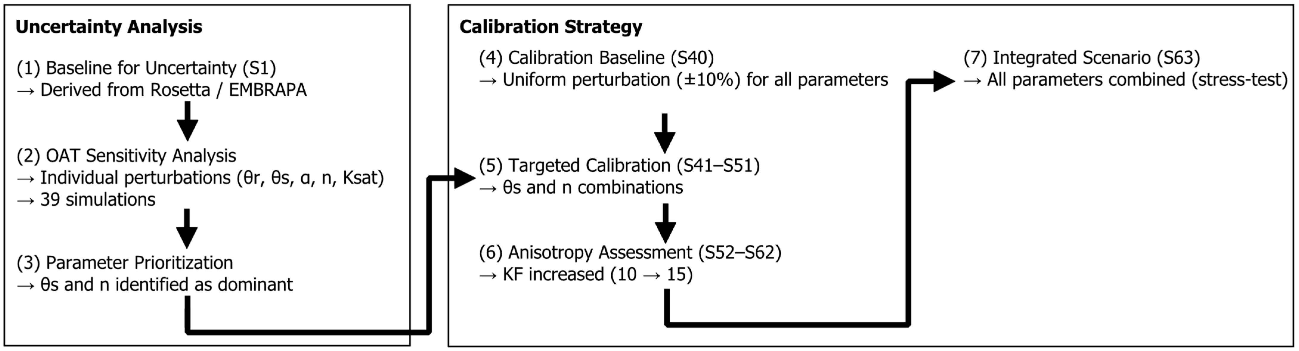
To facilitate understanding of the calibration strategy and its sequential design, a conceptual workflow diagram is presented in Figure 3.

The calibration strategy was designed as a structured and progressive set of experiments, grounded in prior methodological developments and aimed at systematically isolating the effects of soil hydraulic parameters and anisotropy on model performance. The overall design follows the calibration framework established in Sales et al. [16,17], in which computational efficiency and predictive skill are jointly considered when defining optimal parameter perturbation schemes.

As a starting point, a baseline calibration configuration (S40) was defined and adopted as the reference scenario for all subsequent analyses. This configuration corresponds to a uniform ±10% perturbation applied to all VGM parameters, following the multiplicative perturbation strategy proposed in Sales et al. [19] and identified as optimal in Sales et al. [17]. Specifically, the multiplicative factors applied in S40 were ${\theta }_s$ = 1.1, ${\theta }_r$ = 0.9, $\alpha$ = 0.9, $n$ = 1.1, and $K_{sat}$= 1.1. This scenario establishes a consistent reference point against which the effects of targeted parameter adjustments can be evaluated.

The calibration strategy directly builds upon the diagnostic results of the uncertainty analysis presented in Section 2.3. While the OAT framework was adopted to isolate the individual contribution of each VGM parameter to predictive uncertainty, the calibration phase was intentionally designed to move beyond isolated perturbations and to explore targeted parameter interactions identified as hydrologically dominant.

The uncertainty analysis consistently indicated that θ_s and n exert the strongest and most systematic control on simulated streamflow magnitude and variability, as reflected by higher ${\mu }_{Bandwidth}$ values and lower temporal dispersion when compared to ${\theta }_r$, $\alpha$, and $K_{sat}.$ Although the latter parameters exhibited broad physically plausible ranges, their perturbations resulted in comparatively weaker and less consistent impacts on discharge dynamics. Based on this diagnostic evidence, ${\theta }_s$ and $n$ were therefore prioritized for focused calibration.

Accordingly, a new set of calibration scenarios was designed in which θ_s and n were systematically perturbed while all remaining VGM parameters were held fixed at their baseline values (S40). This design choice was directly informed by the uncertainty and sensitivity analysis described in Section 2.3, which identified ${\theta }_s$ and $n$ as the parameters exerting the strongest control on simulated hydrological responses. Based on the parameter ranges explored in that analysis, multiplicative factors for θ_s were progressively increased from 1.1 to 1.3, while $n$ varied from 1.1 up to 1.5. All possible combinations of these perturbation levels were considered, resulting in a total of 11 calibration scenarios (S41–S51), as summarized in

Table 5. Simulation scenarios for soil calibration.

SIM	MST Multiplying Factor					$\mathit{K}\mathit{F}$ Value	Parameter Calibrated
	${\mathit{\theta }}_{\mathit{s}}$	${\mathit{\theta }}_{\mathit{r}}$	$\mathit{\alpha }$	$\mathit{n}$	${\mathit{K}}_{\mathit{s}\mathit{a}\mathit{t}}$
S40	1.1	0.9	0.9	1.1	1.1	10	Calibration baseline
S41	1.2	0.9	0.9	1.1	1.1	10	${\theta }_s\left(+20\mathrm{\%}\right)$
S42	1.3	0.9	0.9	1	1.1	10	${\theta }_s\left(+30\mathrm{\%}\right)$
S43	1.1	0.9	0.9	1.2	1.1	10	$n(+20\mathrm{\%})$
S44	1.2	0.9	0.9	1.2	1.1	10	${\theta }_s\left(+20\mathrm{\%}\right)$, $n(+20\mathrm{\%})$
S45	1.3	0.9	0.9	1.2	1.1	10	${\theta }_s\left(+30\mathrm{\%}\right)$, $n(+20\mathrm{\%})$
S46	1.1	0.9	0.9	1.3	1.1	10	$n(+30\mathrm{\%})$
S47	1.2	0.9	0.9	1.3	1.1	10	${\theta }_s\left(+20\mathrm{\%}\right)$, $n(+30\mathrm{\%})$
S48	1.3	0.9	0.9	1.3	1.1	10	${\theta }_s\left(+30\mathrm{\%}\right)$, $n(+30\mathrm{\%})$
S49	1.1	0.9	0.9	1.5	1.1	10	$n(+50\mathrm{\%})$
S50	1.2	0.9	0.9	1.5	1.1	10	${\theta }_s\left(+20\mathrm{\%}\right)$, $n(+50\mathrm{\%})$
S51	1.3	0.9	0.9	1.5	1.1	10	${\theta }_s\left(+30\mathrm{\%}\right)$, $n(+50\mathrm{\%})$
S52	1.2	0.9	0.9	1.1	1.1	15	${\theta }_s\left(+20\mathrm{\%}\right)$, $KF=15$
S53	1.3	0.9	0.9	1.1	1.1	15	${\theta }_s\left(+30\mathrm{\%}\right)$, $KF=15$
S54	1.1	0.9	0.9	1.2	1.1	15	$n(+20\mathrm{\%})$, $KF=15$
S55	1.2	0.9	0.9	1.2	1.1	15	${\theta }_s\left(+20\mathrm{\%}\right)$, $n(+20\mathrm{\%}),KF=15$
S56	1.3	0.9	0.9	1.2	1.1	15	${\theta }_s\left(+30\mathrm{\%}\right)$, $n(+20\mathrm{\%}),KF=15$
S57	1.1	0.9	0.9	1.3	1.1	15	$n(+30\mathrm{\%})$, $KF=15$
S58	1.2	0.9	0.9	1.3	1.1	15	${\theta }_s\left(+20\mathrm{\%}\right)$, $n(+30\mathrm{\%}),KF=15$
S59	1.3	0.9	0.9	1.3	1.1	15	${\theta }_s\left(+30\mathrm{\%}\right)$, $n(+30\mathrm{\%}),KF=15$
S60	1.1	0.9	0.9	1.5	1.1	15	$n(+50\mathrm{\%})$, $KF=15$
S61	1.2	0.9	0.9	1.5	1.1	15	${\theta }_s\left(+20\mathrm{\%}\right)$, $n(+50\mathrm{\%}),KF=15$
S62	1.3	0.9	0.9	1.5	1.1	15	${\theta }_s\left(+30\mathrm{\%}\right)$, $n(+50\mathrm{\%}),KF=15$
S63	1.3	0.7	0.7	1.5	2	10	${\theta }_s\left(+30\mathrm{\%}\right)$, ${\theta }_r\left(-30\mathrm{\%}\right),$ $\alpha \left(-30\mathrm{\%}\right)$, $n\left(+50\mathrm{\%}\right)$, $K_{sat}\left(+100\mathrm{\%}\right)$

.

Although soil hydraulic anisotropy was not included in the formal uncertainty analysis, previous applications of MOHID-Land have shown that the $KF$ multiplier can significantly affect runoff generation and subsurface flow partitioning, particularly in steep and hydrologically responsive catchments [34]. Therefore, $KF$ was introduced at the calibration stage to evaluate the robustness of the θ_s − n calibration under altered anisotropy conditions. To this end, the ${\theta }_s-n$ combinations defined in scenarios S41–S51 were repeated with $KF$ increased from the default value of 10 to 15, resulting in 11 additional simulations (S52–S62). For consistency, $KF$ remained fixed at 10 in the baseline (S40) and in all ${\theta }_s-n$-only scenarios.

Finally, a comprehensive calibration scenario (S63) was defined as an exploratory stress test rather than a candidate optimal solution. In this scenario, all VGM parameters were simultaneously adjusted according to the uncertainty ranges and sensitivity patterns identified in Section 2.3, while $KF$ was maintained at its default value. The purpose of this configuration is to assess the cumulative and potentially compensatory effects of simultaneous parameter perturbations, thereby providing a reference envelope for model behavior under maximally adjusted soil hydraulic conditions.

In total, the calibration phase comprised 24 systematically designed scenarios (S40–S63). This experimental framework enables a clear separation between (i) baseline model behavior, (ii) the isolated effects of the most sensitive soil hydraulic parameters, (iii) the combined influence of parameter variation and hydraulic anisotropy, and (iv) an integrated soil parameter configuration. All calibration simulations were performed for the period 2006–2008, with the year 2006 adopted as a warm-up period, consistent with the uncertainty experiments.

2.5. Validation Scenarios

Following the uncertainty analysis and soil calibration, a validation period was implemented to assess model performance under independent conditions not included in the calibration process. Three key scenarios were selected for this validation phase: (i) the reference scenario (S1), which employed uncalibrated input parameters obtained directly from EMBRAPA and the Rosetta model; (ii) scenario S40, in which all VGM parameters were uniformly perturbed by ±10%, following the methodology proposed by Sales et al. [19] and Sales et al. [20]; and (iii) a performance-optimized scenario that applied the best combination of multiplicative factors for ${\theta }_s$, $n$, and $KF$, as identified during the calibration stage.

The validation period spanned from 2009 to 2016, covering eight consecutive years of continuous hydrological data. This interval was selected due to the availability of consistent and uninterrupted observed records, ensuring a robust basis for model evaluation. Data from 2017 to 2018 were excluded because of gaps and inconsistencies in the observed time series. The analysis considered seasonal variability, with the year divided into wet (October to March) and dry (April to September) seasons, in line with the rainfall regime typical of tropical watersheds.

2.6. Exploratory Calibration Experiment with Surface Hydraulic Parameters

Although the primary focus of this research is the calibration of soil hydraulic parameters, an additional exploratory experiment was conducted to evaluate the feasibility of extending the calibration to surface and channel hydraulic characteristics. Specifically, the Manning roughness coefficient for the watershed surface, the Manning coefficient for the main channel, and the geometries of the river cross-sections were jointly included in this analysis.

These parameters were selected due to their well-established influence on surface runoff generation and concentrated flow within channels. The magnitude and direction of the parameter adjustments were guided by Oliveira et al. [18]. Accordingly, both the watershed and channel Manning coefficients were increased by 50%.

With respect to the river cross-sections, Oliveira et al. [18] tested increases of 25% in channel width and 100% in depth, which resulted in higher streamflow values. However, since the present model exhibited some degree of flow overestimation at specific locations, a more conservative strategy was adopted. Thus, reductions were applied to the channel dimensions to mitigate excessive simulated discharge.

Consistent with the previous methodological stages, the simulation period was divided into three phases: 2006 was defined as the warm-up period, 2007–2008 as the calibration period, and 2009–2016 as the validation period.

2.7. Model Performance

Model performance was evaluated using a combination of quantitative metrics and diagnostic tools. Quantitative agreement between observed and simulated streamflow was assessed using the Nash–Sutcliffe efficiency ($NSE$) coefficient and the percentage bias ($PBIAS$), defined in Equations (11) and (12), respectively:

$$NSE=1-\left[{\displaystyle \frac{\sum _{i=1}^p{(Q_i^{obs}-Q_i^{sim})}^2}{\sum _{i=1}^p{(Q_i^{obs}-Q_{mean}^{obs})}^2}}\right]$$

(11)

$$PBIAS={\displaystyle \frac{\sum _{i=1}^p(Q_i^{sim}-Q_i^{obs})}{\sum _{i=1}^p{Q}_i^{obs}}}\times 100$$

(12)

where $Q_i^{sim}$ is the simulated flow for day $i$ [m³/s]; $Q_i^{obs}$ is the observed flow on day $i$ [m³/s]; $Q_{mean}^{obs}$ is the observed mean flow for the period under consideration [m³/s]; $Q_{mean}^{sim}$ is the simulated mean flow for the period under consideration [m³/s]; and $p$ is the total number of days in that same period.

The $NSE$ evaluates model accuracy by comparing the variance of the simulation residuals with the variance of the observed data. Its values range from negative infinity to 1, with values closer to 1 indicating better model performance. An $NSE$ value lower than zero suggests that the observed mean is a better predictor than the model simulation. For streamflow simulations, $NSE$ values above 0.80 are classified as “Very Good”, values between 0.70 and 0.80 as “Good”, values between 0.50 and 0.70 as “Satisfactory”, and values below 0.50 as “Not Satisfactory” [53].

The $PBIAS$ metric measures the average tendency of the simulated values to be larger or smaller than their observed counterparts, with an optimal value of zero. Positive $PBIAS$ values indicate model overestimation, whereas negative values indicate underestimation. For streamflow, $PBIAS$ values within ±5 are considered “Very Good”, ±5 to ±10 “Good”, ±10 to ±15 “Satisfactory”, and values exceeding ±15 “Not Satisfactory” [53].

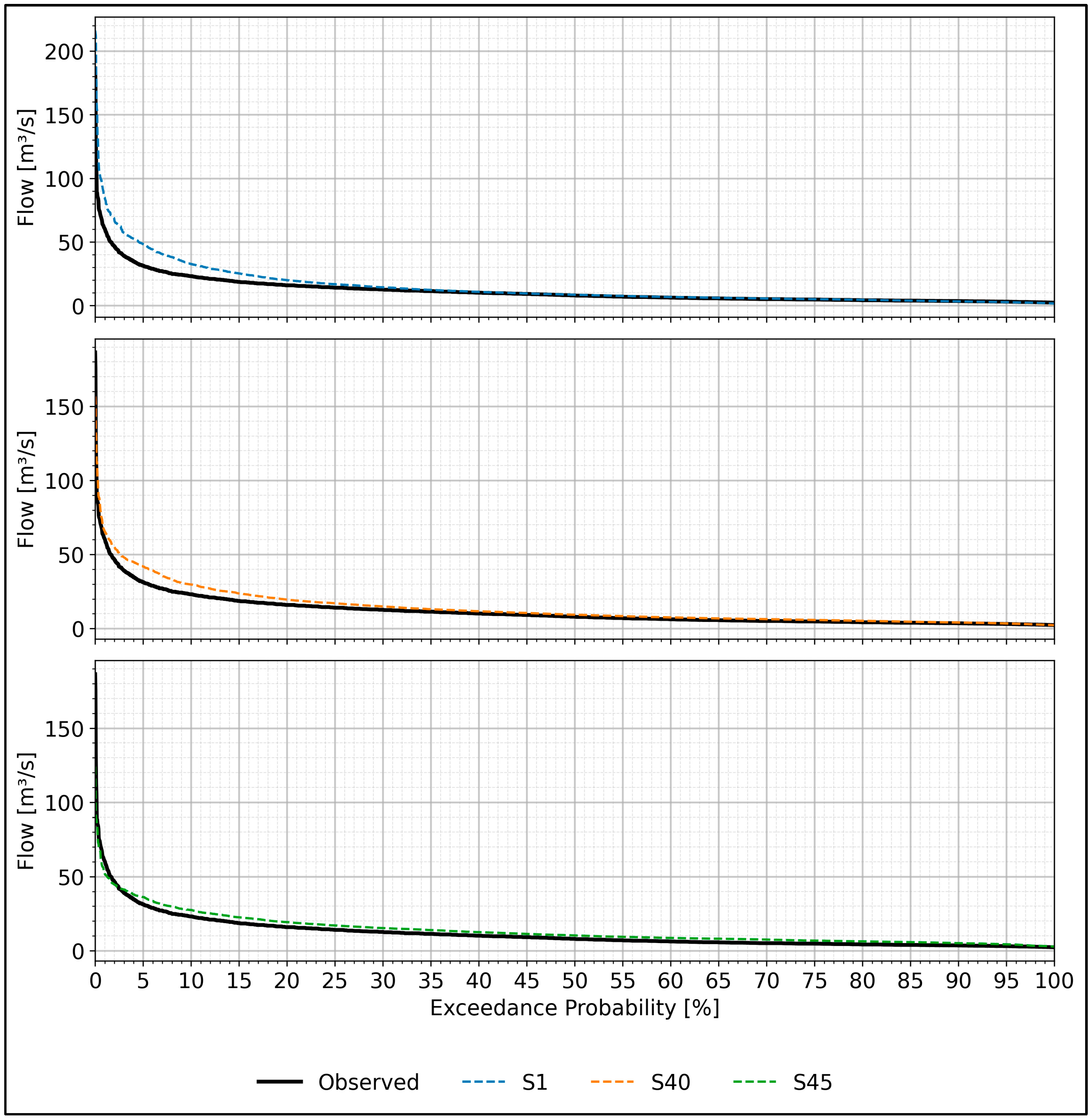
For the validation phase, the Flow Duration Curve (FDC) was used as an additional diagnostic tool to evaluate calibration effectiveness by visually comparing simulated and observed streamflow over the full range of flow conditions, following the approach of Oliveira et al. [18]. The FDC analysis enabled the identification of discrepancies across low, medium, and high flows, thereby supporting the assessment of different parameterizations. The close agreement between the observed and simulated FDCs obtained with the final model setup indicates an improved representation of streamflow dynamics across all flow regimes.

3. Results

3.1. Streamflow Uncertainty Based on VGM Parameter Perturbation

3.1.1. Effect of ${\theta }_s$ Variation on Flow Dynamics

The results indicate that variation in saturated water content (${\theta }_s$) produces the most pronounced performance changes during the wet season, primarily reflected in peak-flow metrics. In the reference configuration (S1; ${\theta }_s$= 0.5017 m³ m⁻³), the model exhibits clear deficiencies under high-flow conditions, with wet-season $NSE$ = −0.21 and $PBIAS$ = 54.73% (

Table 6. ${\theta }_s$ scenarios performance.

Simulation	Mean of  ${\mathit{\theta }}_{\mathit{s}}$ [m3/m3]	$\mathit{N}\mathit{S}\mathit{E}$			$\mathit{P}\mathit{B}\mathit{I}\mathit{A}\mathit{S}$
		Full Period	Wet Season	Dry Season	Full Period	Wet Season	Dry Season
S2	0.3512	−0.42	−0.73	0.48	37.44	66.22	−22.59
S3	0.4014	−0.26	−0.54	0.53	36.13	62.14	−18.10
S4	0.4515	−0.11	−0.36	0.57	34.98	58.23	−13.51
S1	0.5017	0.01	−0.21	0.60	34.06	54.73	−9.02
S5	0.5519	0.13	−0.06	0.61	33.10	51.22	−4.68
S6	0.6021	0.24	0.08	0.63	31.84	47.42	−0.66
S7	0.6522	0.34	0.21	0.63	30.13	43.17	2.94

), indicating substantial overestimation of flood peaks.

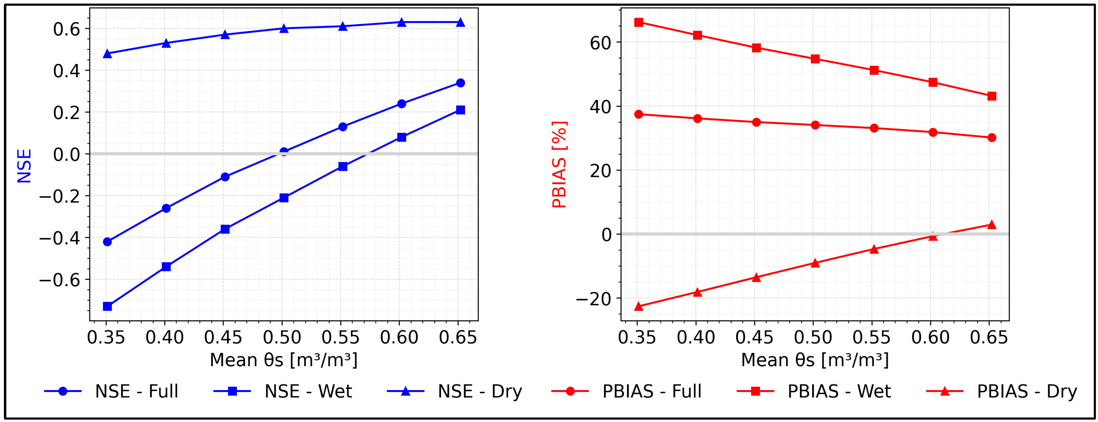
As shown in Table 6, progressive increases in ${\theta }_s$ from 0.3512 m³ m⁻³ (S2) to 0.6522 m³ m⁻³ (S7) result in systematic and monotonic improvements across all temporal subsets. Over the full simulation period, $NSE$ increases steadily from −0.42 (S2) to 0.34 (S7), representing a total gain of 0.76 units. Concurrently, full-period $PBIAS$ decreases from 37.44% to 30.13%, reflecting a 7.31 percentage-point reduction.

The wet season exhibits the strongest sensitivity. $NSE$ increases from −0.73 (S2) to 0.21 (S7), corresponding to an improvement of 0.94 units. In parallel, wet-season $PBIAS$ decreases from 66.22% to 43.17%, representing a reduction of 23.05 percentage points. Notably, the transition from negative to positive wet-season $NSE$ occurs between S5 (−0.06) and S6 (0.08), indicating a threshold response within the tested ${\theta }_s$ range.

The incremental performance gains diminish at higher ${\theta }_s$ values. Between S6 and S7, wet-season $NSE$ increases by only 0.13 units (0.08 to 0.21), compared to earlier increments exceeding 0.15–0.19 units between successive scenarios. A similar attenuation is observed for $PBIAS$ reduction, suggesting reduced marginal gains at elevated ${\theta }_s$ levels.

Dry-season metrics display a more moderate but consistent response. $NSE$ increases from 0.48 (S2) to 0.63 (S7), yielding a total improvement of 0.15 units. Unlike the wet season, dry-season $NSE$ remains positive across all scenarios and stabilizes at 0.63 between S6 and S7. Dry-season $PBIAS$ shifts from −22.59% (underestimation) to 2.94% (slight overestimation), crossing zero between S6 (−0.66%) and S7 (2.94%). This shift indicates a progressive reduction in low-flow underestimation as ${\theta }_s$ increases.

The structured response across scenarios is illustrated in Figure 4, which shows an approximately linear relationship between ${\theta }_s$ and both $NSE$ and $PBIAS$ for the full and wet-season periods. The slope of improvement is steeper for wet-season $NSE$ compared to dry-season $NSE$, corroborating the stronger seasonal sensitivity observed in Table 6.

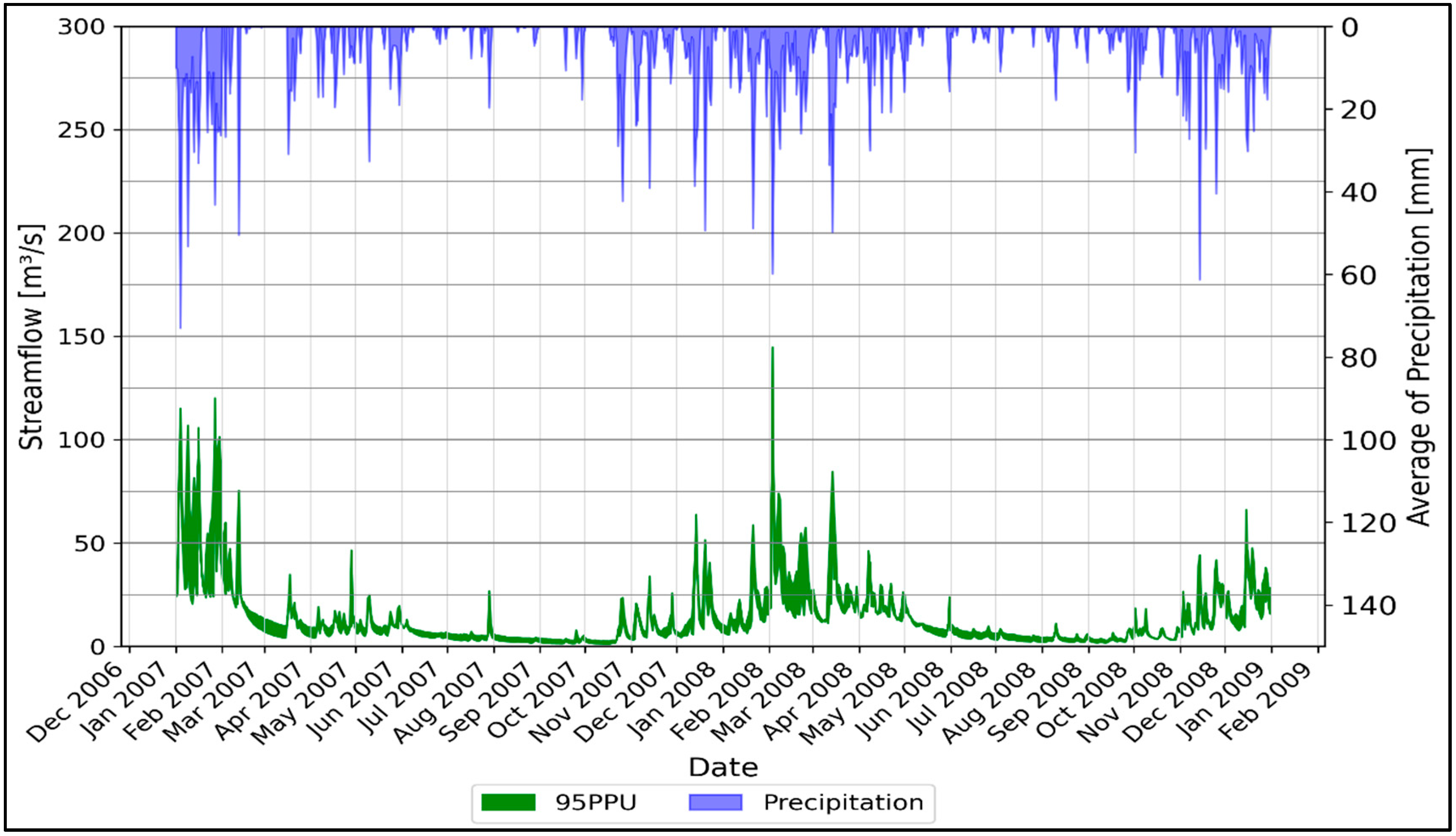
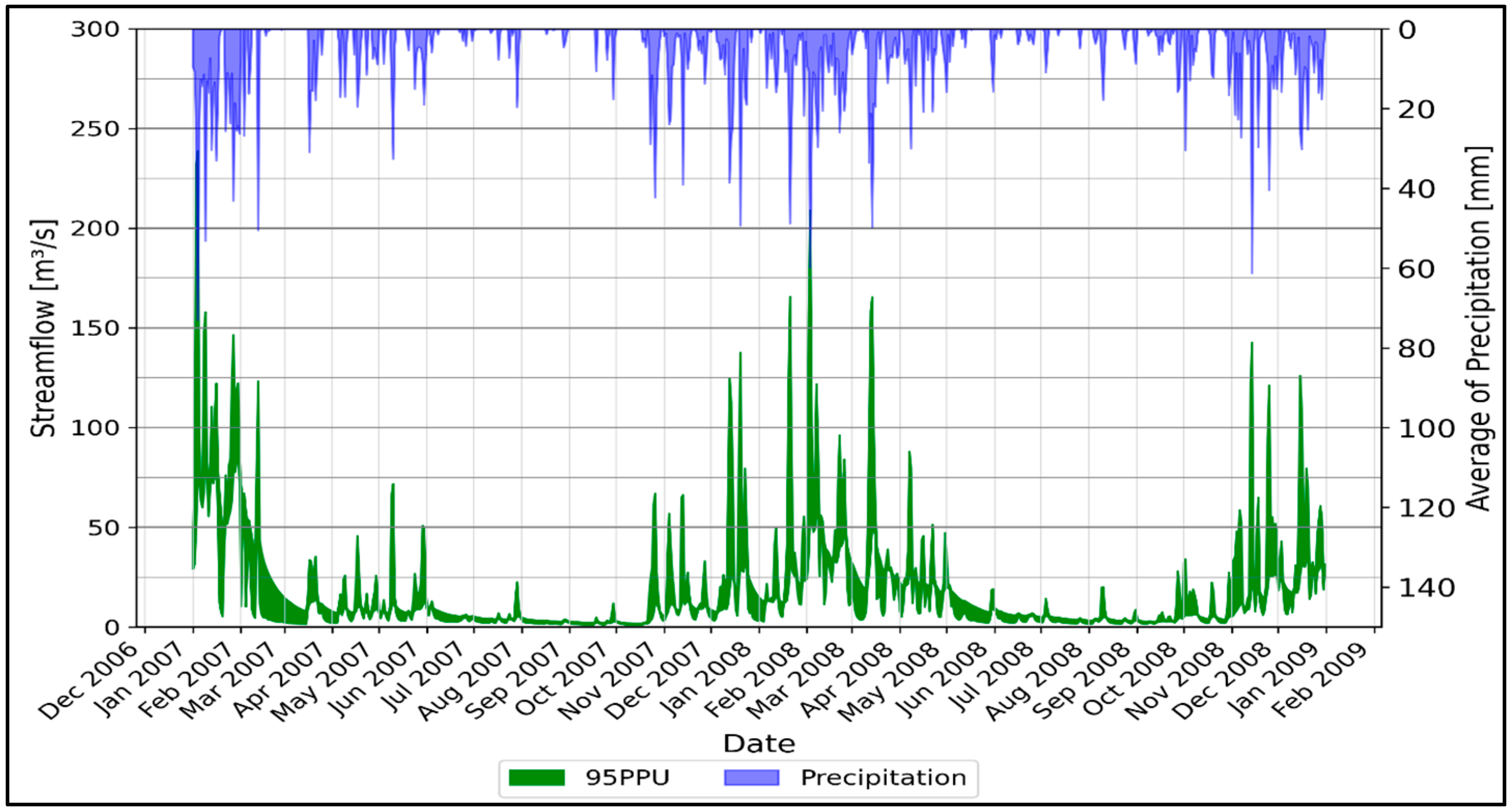
The seasonal differentiation in performance is mirrored in the 95% prediction uncertainty (95PPU) analysis (Figure 5). The uncertainty envelope expands considerably during high-flow periods, particularly in months characterized by clustered precipitation events, where simulated peak dispersion increases visibly.

Quantitatively, the wet season exhibits a mean bandwidth of 6.16 m³ s⁻¹ with a coefficient of variation of 146.20%, indicating substantial predictive spread during peak-flow conditions. In contrast, the dry season shows markedly narrower envelopes (${\mu }_{Bandwidth}= 2.23 {\mathrm{m}}^3{\mathrm{s}}^{-1}; CV = 34.89\%$), consistent with the smaller variation in $NSE$ across ${\theta }_s$ scenarios under low-flow conditions.

For the entire simulation period, the mean bandwidth equals 4.19 m³ s⁻¹ ($CV = 159.32\%$). The larger full-period $CV$ relative to the seasonal values reflects the influence of episodic peak events, which produce short-duration but high-magnitude envelope expansions visible in Figure 5.

During recession periods, the 95PPU envelope narrows and closely follows observed discharge, indicating reduced parametric dispersion under low-flow conditions. Conversely, during major runoff events, the envelope broadens substantially, confirming that ${\theta }_s$ variation primarily affects predictive spread during peak-flow episodes.

3.1.2. Effect of ${\theta }_r$ Variation on Flow Dynamics

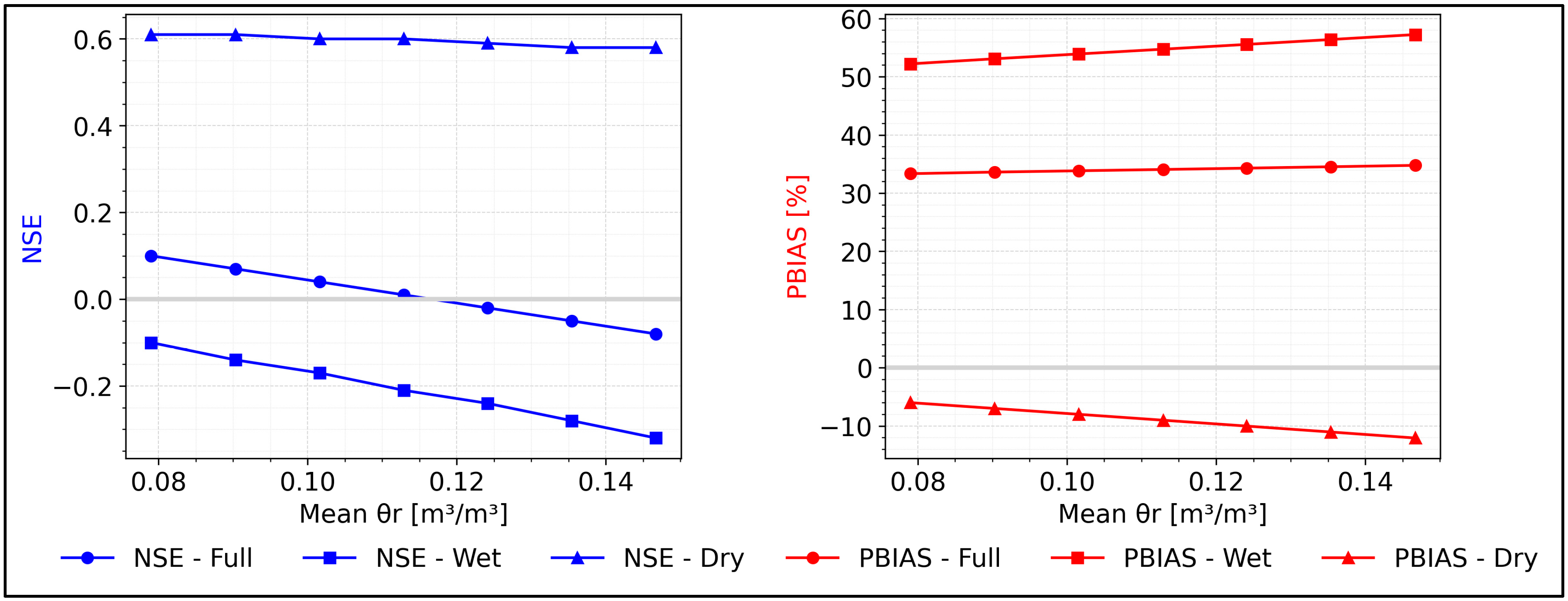
In contrast to ${\theta }_s$, where performance improves with increasing parameter values, ${\theta }_r$ exhibits improvement toward its lower bound; nevertheless, the associated performance changes are minor. Relative to the baseline simulation (S1), full-period $NSE$ varies symmetrically within ±0.09, confirming the weak structural influence of ${\theta }_r$ on model response.

As shown in

Table 7. ${\theta }_r$ scenarios performance.

Simulation	Mean of ${\mathit{\theta }}_{\mathit{r}}$ [m3/m3]	$\mathit{N}\mathit{S}\mathit{E}$			$\mathit{P}\mathit{B}\mathit{I}\mathit{A}\mathit{S}$
		Full Period	Wet Season	Dry Season	Full Period	Wet Season	Dry Season
S8	0.0790	0.10	−0.10	0.61	33.34	52.21	−6.00
S9	0.0903	0.07	−0.14	0.61	33.61	53.08	−7.00
S10	0.1016	0.04	−0.17	0.60	33.84	53.91	−8.01
S1	0.1129	0.01	−0.21	0.60	34.06	54.73	−9.02
S11	0.1241	−0.02	−0.24	0.59	34.29	55.55	−10.03
S12	0.1354	−0.05	−0.28	0.58	34.53	56.39	−11.05
S13	0.1467	−0.08	−0.32	0.58	34.77	57.24	−12.08

and Figure 6, increasing ${\theta }_r$ from 0.0790 to 0.1467 m³ m⁻³ produces a systematic and approximately linear degradation of model performance across all evaluation periods. Over the full simulation period, $NSE$ declines from 0.10 (S8) to −0.08 (S13), corresponding to a total variation of 0.18 units across the entire tested interval. Relative to the central configuration (S1; ${\theta }_r$ = 0.1129 m³ m⁻³; $NSE$ = 0.01), the maximum improvement achieved at the lower bound (S8) is limited to +0.09 units, whereas the maximum degradation reaches −0.09 units at the upper bound (S13), indicating symmetric and small-amplitude variation around the baseline. $PBIAS$ exhibits a similarly gradual response, increasing from 33.34% to 34.77%, a total change of only 1.43 percentage points. The near-uniform slopes observed in Figure 6 confirm a proportional and nearly linear relationship between ${\theta }_r$ and performance metrics, with no inflection points or internal optima within the tested range.

Seasonal results follow the same structured but limited pattern. During the wet season, $NSE$ decreases from −0.10 to −0.32 (Δ = 0.22) and $PBIAS$ increases from 52.21% to 57.24% (Δ = 5.03%), representing the largest observed sensitivity; however, the response remains monotonic and moderate in magnitude. In the dry season, variations are even smaller, with $NSE$ declining from 0.61 to 0.58 (Δ = 0.03) and $PBIAS$ shifting from −6.00% to −12.08%.

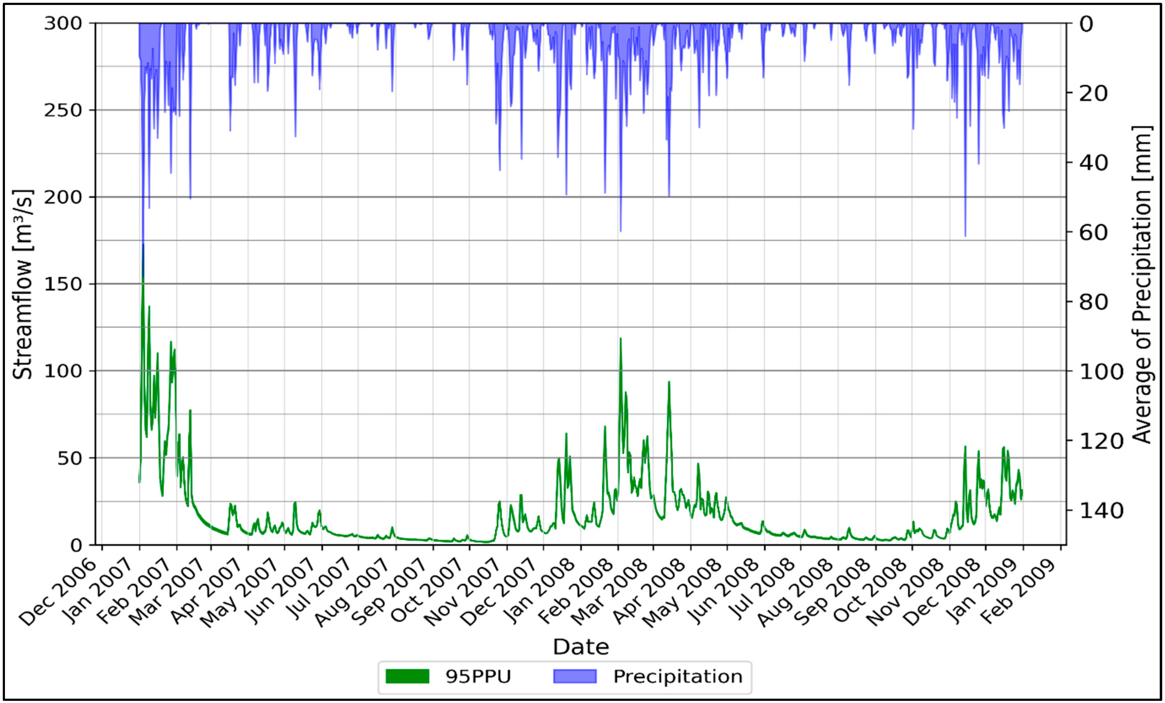
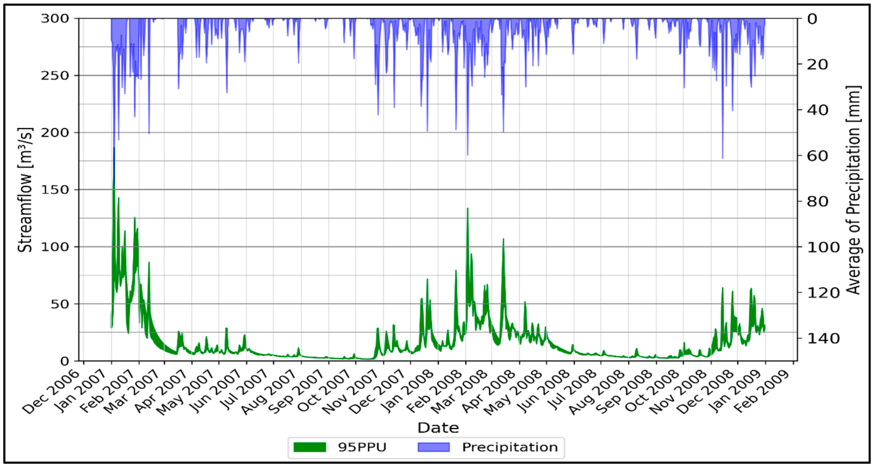
Uncertainty analysis based on the 95PPU envelope (Figure 7) further confirms the low sensitivity of ${\theta }_r$. Across the full period, uncertainty bands remain narrow (${\mu }_{Bandwidth}= 0.96 {\mathrm{m}}^3{\mathrm{s}}^{-1}),$ despite high relative variability ($CV = 162.93\%$). Seasonal differences are minor, with slightly wider bands during the wet season (${\mu }_{Bandwidth}=1.40 {\mathrm{m}}^3{\mathrm{s}}^{-1}; CV = 152.18\%$) and narrower bands during the dry season (${\mu }_{Bandwidth}=0.53 {\mathrm{m}}^3{\mathrm{s}}^{-1}; CV = 33.89\%$).

Overall, the results indicate that ${\theta }_r$ exerts consistent but weak control on streamflow metrics compared to ${\theta }_s$.

3.1.3. Effect of $\alpha$ Variation on Flow Dynamics

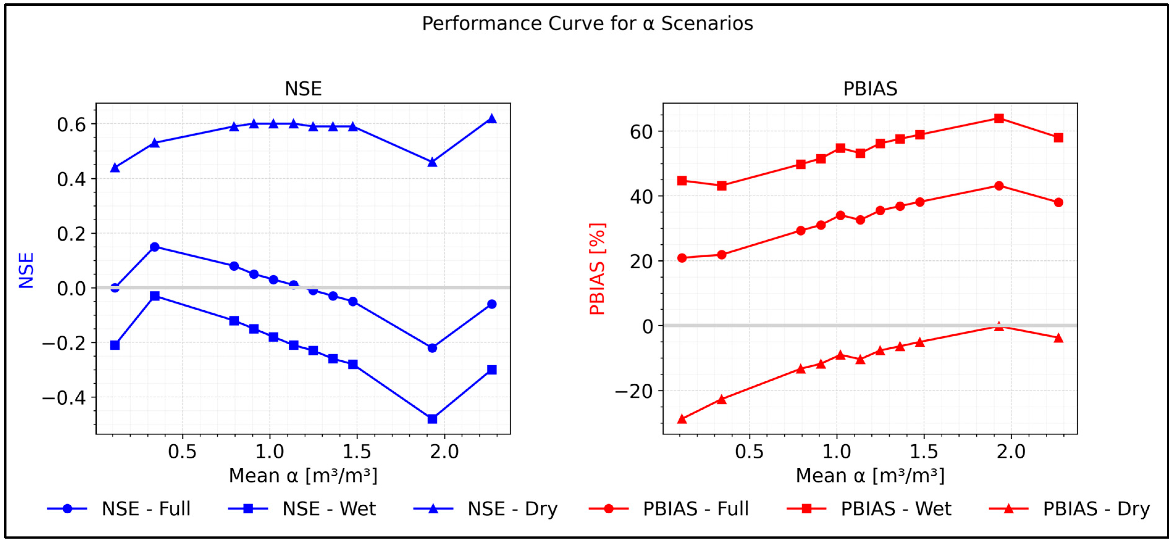
As shown in

Table 8. $\alpha$ scenarios performance.

Simulation	Mean of $\mathit{\alpha }$ [m−1]	$\mathit{N}\mathit{S}\mathit{E}$			$\mathit{P}\mathit{B}\mathit{I}\mathit{A}\mathit{S}$
		Full Period	Wet Season	Dry Season	Full Period	Wet Season	Dry Season
S14	0.113	0.00	−0.21	0.44	20.89	44.70	−28.77
S15	0.340	0.15	−0.03	0.53	21.84	43.19	−22.69
S16	0.794	0.08	−0.12	0.59	29.31	49.74	−13.31
S17	0.908	0.05	−0.15	0.60	31.00	51.51	−11.78
S18	1.021	0.03	−0.18	0.60	34.06	54.73	−9.02
S1	1.135	0.01	−0.21	0.60	32.57	53.16	−10.37
S19	1.248	−0.01	−0.23	0.59	35.48	56.17	−7.67
S20	1.362	−0.03	−0.26	0.59	36.84	57.56	−6.37
S21	1.475	−0.05	−0.28	0.59	38.14	58.86	−5.05
S22	1.929	−0.22	−0.48	0.46	43.16	63.94	−0.17
S23	2.270	−0.06	−0.30	0.62	38.01	58.02	−3.73

and Figure 8, variations in $\alpha$ produce a structured but limited response relative to the baseline simulation (S14; $\alpha$ = 0.113 m⁻¹). For the full period, the maximum improvement occurs at $\alpha$ = 0.340 (S15), where $NSE$ increases from 0.00 to 0.15, representing a punctual gain of 0.15 units. Beyond this value, $NSE$ declines progressively, reaching −0.22 at $\alpha$ = 1.929 (S22), which corresponds to a degradation of 0.22 units relative to the baseline and 0.37 units relative to the local maximum. At the upper boundary ($\alpha$ = 2.270), $NSE$ partially recovers to −0.06, but remains below the best observed performance. This pattern indicates that $\alpha$ exhibits greater potential to degrade model performance than to improve it within the tested range. Consistently, $PBIAS$ increases from 20.89% (S14) to 43.16% (S22), with only partial reduction at the highest $\alpha$ value, reinforcing the predominance of performance deterioration at larger parameter values.

Between $\alpha$ = 0.794 and $\alpha$ = 1.475 (S16–S21), both $NSE$ and $PBIAS$ display an approximately linear and gradual behavior. Within this intermediate range, $NSE$ declines steadily from 0.08 to −0.05, while $PBIAS$ increases from 29.31% to 38.14%, without abrupt inflections. This near-linear segment suggests a proportional response to parameter perturbation over a substantial portion of the explored space. Seasonal analysis reinforces the limited magnitude of sensitivity. During the wet season, $NSE$ varies between −0.03 and −0.48, with progressive degradation up to $\alpha$ = 1.929 and partial recovery thereafter, while dry-season $NSE$ increases from 0.44 to 0.62, with a localized decrease at $\alpha$ = 1.929. Although directional differences exist between wet and dry regimes, the absolute variations remain moderate, and no stable internal optimum emerges. Overall, $\alpha$ variation produces regime-dependent but comparatively marginal performance changes within the tested bounds, indicating limited structural control over streamflow simulation relative to parameters exhibiting clearer optimal responses.

Uncertainty analysis based on the 95PPU envelope (Figure 9) shows intermediate but unstable sensitivity. Across the full period, the mean uncertainty bandwidth is 4.08 m³ s⁻¹ ($CV = 87.25\%$), wider than that observed for ${\theta }_r$ but lacking the strong seasonal structuring seen for ${\theta }_s$. Wet-season bands widen moderately (5.31 m³ s⁻¹), while dry-season bands are narrower (2.86 m³ s⁻¹), indicating variability without clear directional dominance.

3.1.4. Effect of $n$ Variation on Flow Dynamics

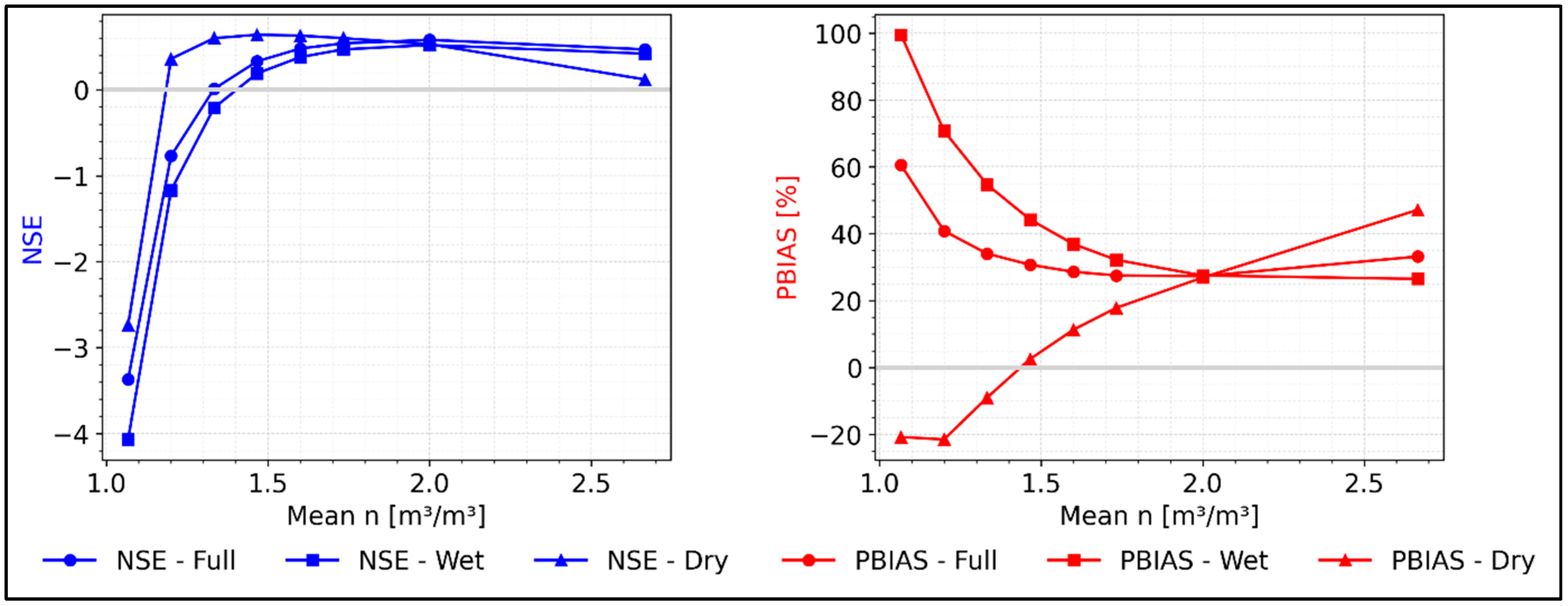
Among the VGM parameters evaluated, $n$ exhibits a systematic and internally consistent performance response within the tested range. As shown in

Table 9. $n$ scenarios performance.

Simulation	Mean of $\mathit{n}$ [Dimensionless]	$\mathit{N}\mathit{S}\mathit{E}$			$\mathit{P}\mathit{B}\mathit{I}\mathit{A}\mathit{S}$
		Full Period	Wet Season	Dry Season	Full Period	Wet Season	Dry Season
S24	1.067	−3.37	−4.07	−2.74	60.53	99.51	−20.78
S25	1.200	−0.77	−1.17	0.36	40.84	70.74	−21.53
S1	1.333	0.01	−0.21	0.60	34.06	54.73	−9.02
S26	1.466	0.33	0.19	0.64	30.73	44.26	2.50
S27	1.600	0.48	0.38	0.63	28.61	36.93	11.27
S28	1.733	0.54	0.47	0.60	27.53	32.18	17.84
S29	2.000	0.58	0.52	0.53	27.31	27.51	26.89
S30	2.666	0.47	0.42	0.12	33.19	26.49	47.15

and Figure 10, model efficiency follows a non-linear but organized trajectory across the tested range, characterized by (i) an initial monotonic improvement, (ii) a clearly identifiable optimum, and (iii) progressive deterioration beyond that range.

Across the full simulation period, increasing $n$ from 1.067 (S24) to 2.000 (S29) results in a substantial and continuous improvement in $NSE$ (from −3.37 to 0.58) and a concomitant reduction in $PBIAS$ (from 60.53% to 27.31%). This progression is not oscillatory or irregular; instead, it displays a consistent directional trend up to $n$ ≈ 2.0.

For $n$ = 2.666 (S30), performance declines ($NSE$ = 0.47; $PBIAS$ = 33.19%), indicating that the response does not increase indefinitely. Rather than suggesting asymptotic growth, the results support the existence of an internal optimum within the tested interval. Thus, the response pattern is non-linear and characterized by a bounded optimal range within the explored parameter space.

Sensitivity to $n$ is most pronounced during the wet season. NSE improves markedly from −4.07 (S24) to 0.52 (S29), while $PBIAS$ decreases from 99.51% to approximately 27%. The magnitude of this improvement indicates that the primary gains associated with increasing $n$ are linked to the simulation of higher-flow conditions.

Notably, marginal gains decrease near the optimum. The improvement between $n$ = 1.733 (S28) and $n$ = 2.000 (S29) is comparatively small relative to earlier increments, indicating diminishing performance gains within that range. However, no formal asymptotic behavior was tested; therefore, the evidence supports saturation within the explored interval rather than a true asymptote.

In contrast, dry-season performance reveals a distinct regime-dependent response. $NSE$ reaches higher values at intermediate $n$ (1.466–1.600) and declines steadily for larger values, reaching 0.12 at $n$ = 2.666. Similarly, $PBIAS$ shifts from underestimation (−20.78%) toward substantial overestimation (47.15%) as $n$ increases.

This behavior indicates a seasonal trade-off: parameter values that enhance peak-flow representation may compromise baseflow simulation when exceeding the optimal range.

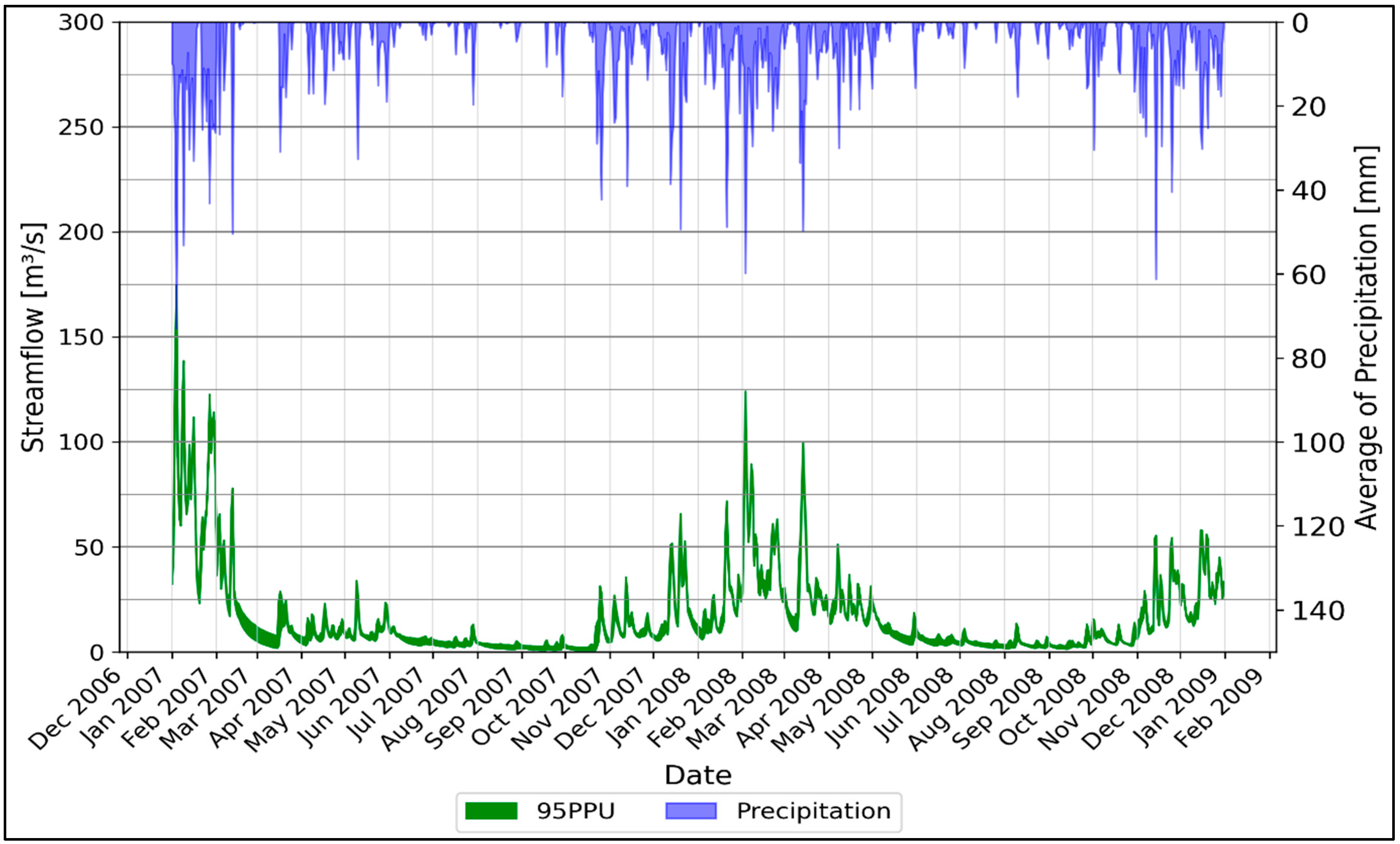
The 95PPU analysis (Figure 11) quantifies the magnitude and variability of predictive dispersion associated with variations in $n$. Over the full simulation period, the mean uncertainty bandwidth reaches 17.56 m³ s⁻¹, with a $CV$ of 123.36%, indicating substantial temporal fluctuation in envelope amplitude. The uncertainty band expands markedly during peak-flow episodes and contracts during recession periods, evidencing substantial temporal variability in predictive dispersion across the simulation period.

Seasonal segmentation highlights stronger dispersion during the wet period, where the mean bandwidth increases to 25.28 m³ s⁻¹ ($CV = 110.20\%$), representing the largest uncertainty magnitude observed. In contrast, the dry season presents a reduced mean width of 9.86 m³ s⁻¹, although the $CV$ remains relatively high (68.42%), indicating persistent variability despite lower absolute dispersion. These values confirm seasonal differentiation in uncertainty magnitude, with maximum dispersion during the wet period and reduced, though still variable, dispersion during the dry season.

Based strictly on the results presented in Table 9, the response of $n$ can be described as systematic, non-linear, and characterized by a bounded optimal range within the tested interval. The results do not support indefinite improvement nor random variability; rather, they reveal a coherent parametric sensitivity pattern with a well-defined internal maximum within the tested interval.

Importantly, the conclusions are restricted to the explored parameter space and should not be generalized beyond it without additional testing.

3.1.5. Effect of $K_{sat}$ Variation on Flow Dynamics

Table 10. $K_{sat}$ scenarios performance.

Simulation	Mean of ${\mathit{K}}_{\mathit{s}\mathit{a}\mathit{t}}$ [cm/day]	$\mathit{N}\mathit{S}\mathit{E}$			$\mathit{P}\mathit{B}\mathit{I}\mathit{A}\mathit{S}$
		Full Period	Wet Season	Dry Season	Full Period	Wet Season	Dry Season
S31	10.019	−2.63	−3.32	−1.42	57.49	90.08	−10.47
S32	70.135	−0.22	−0.50	0.53	37.81	60.04	−8.55
S33	80.154	−0.13	−0.38	0.56	36.55	58.23	−8.67
S34	90.174	−0.05	−0.28	0.58	35.17	56.27	−8.83
S1	100.193	0.01	−0.21	0.60	34.06	54.73	−9.02
S35	110.212	0.06	−0.15	0.61	33.08	53.35	−9.19
S36	120.232	0.10	−0.10	0.62	32.18	52.10	−9.34
S37	130.251	0.13	−0.06	0.62	31.42	51.04	−9.49
S38	200.386	0.25	0.09	0.64	27.50	45.67	−10.40
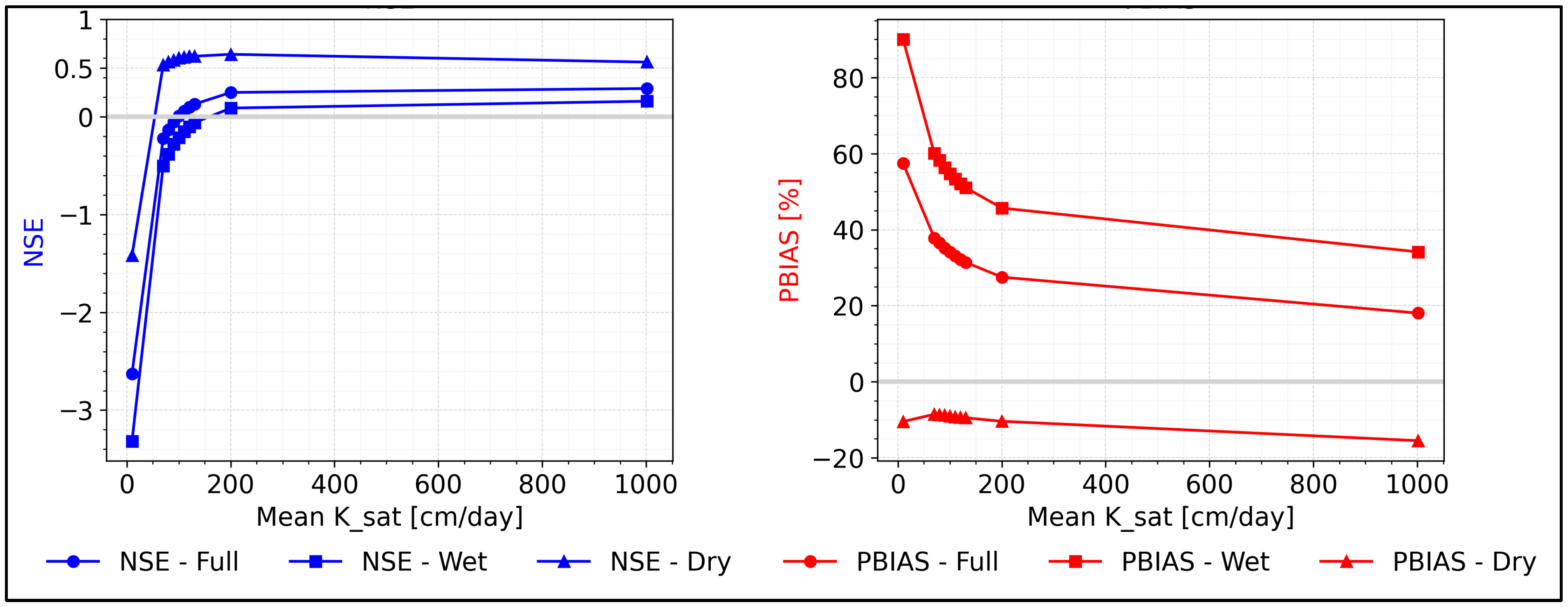
S39	1001.931	0.29	0.16	0.56	18.05	34.13	−15.50

and Figure 12 reveal that ${ K}_{sat}$ controls model performance through a markedly non-linear, threshold-dependent response characterized by three distinct regimes: (i) extreme degradation at very low-conductivity, (ii) rapid recovery within a transitional range, and (iii) diminishing returns beyond an intermediate threshold. The lowest conductivity scenario (S31; 10.019 cm day⁻¹) produces severe deterioration, with full-period $NSE$ = −2.63 and wet-season $NSE$ = −3.32, far outside the range observed for any other parameter tested. Relative to the baseline (S1; 100.193 cm day⁻¹; $NSE$ = 0.01), this corresponds to a degradation of −2.64 $NSE$ units, demonstrating that insufficient conductivity destabilizes the hydrological balance rather than merely reducing efficiency.

The recovery between 10 and 70 cm day⁻¹ is abrupt and disproportionate. Increasing ${ K}_{sat}$ from 10.019 (S31) to 70.135 cm day⁻¹ (S32) improves full-period $NSE$ from −2.63 to −0.22, a gain of +2.41 units, representing more than 90% of the total recoverable improvement observed across the entire parameter range (−2.63 to +0.29). A similar pattern is observed for wet-season $NSE$ (−3.32 to −0.50; +2.82 units). This steep slope in the lower segment of the curve indicates high parameter elasticity under low-conductivity conditions. Visually, Figure 12 confirms a sharp curvature in this interval, contrasting with the flattening observed thereafter.

Between approximately 80 and 130 cm day⁻¹ (S33–S37), the response becomes quasi-linear and progressively attenuated. In this interval, full-period $NSE$ increases modestly from −0.13 to 0.13 (Δ = 0.26), and wet-season $NSE$ from −0.38 to −0.06 (Δ = 0.32). The incremental gains per 10 cm day⁻¹ decrease steadily, indicating a reduction in marginal sensitivity. This transitional band contains the baseline (S1), suggesting that the calibrated configuration already lies within a near-stable performance plateau.

Beyond approximately 200 cm day⁻¹, the response approaches an asymptotic regime. From 200.386 cm day⁻¹ (S38) to 1001.931 cm day⁻¹ (S39), full-period $NSE$ increases only from 0.25 to 0.29 (Δ = 0.04), despite a fivefold increase in conductivity. Wet-season $NSE$ improves from 0.09 to 0.16 (Δ = 0.07), while dry-season $NSE$ decreases from 0.64 to 0.56 (Δ = −0.08), indicating that very high conductivities introduce trade-offs between seasonal regimes rather than systematic gains. This behavior is clearly visible in Figure 12, where the curves flatten and, in the dry season, slightly decline at the upper boundary.

$PBIAS$ follows the same structural pattern. The largest correction occurs between S31 and S32, where wet-season $PBIAS$ drops from 90.08% to 60.04% (−30.04 percentage points). Subsequent reductions become progressively smaller, reaching 34.13% at the highest conductivity. Notably, the largest proportional improvements in bias correction occur within the same low-conductivity interval where $NSE$ curvature is steepest, reinforcing the existence of a dominant threshold effect.

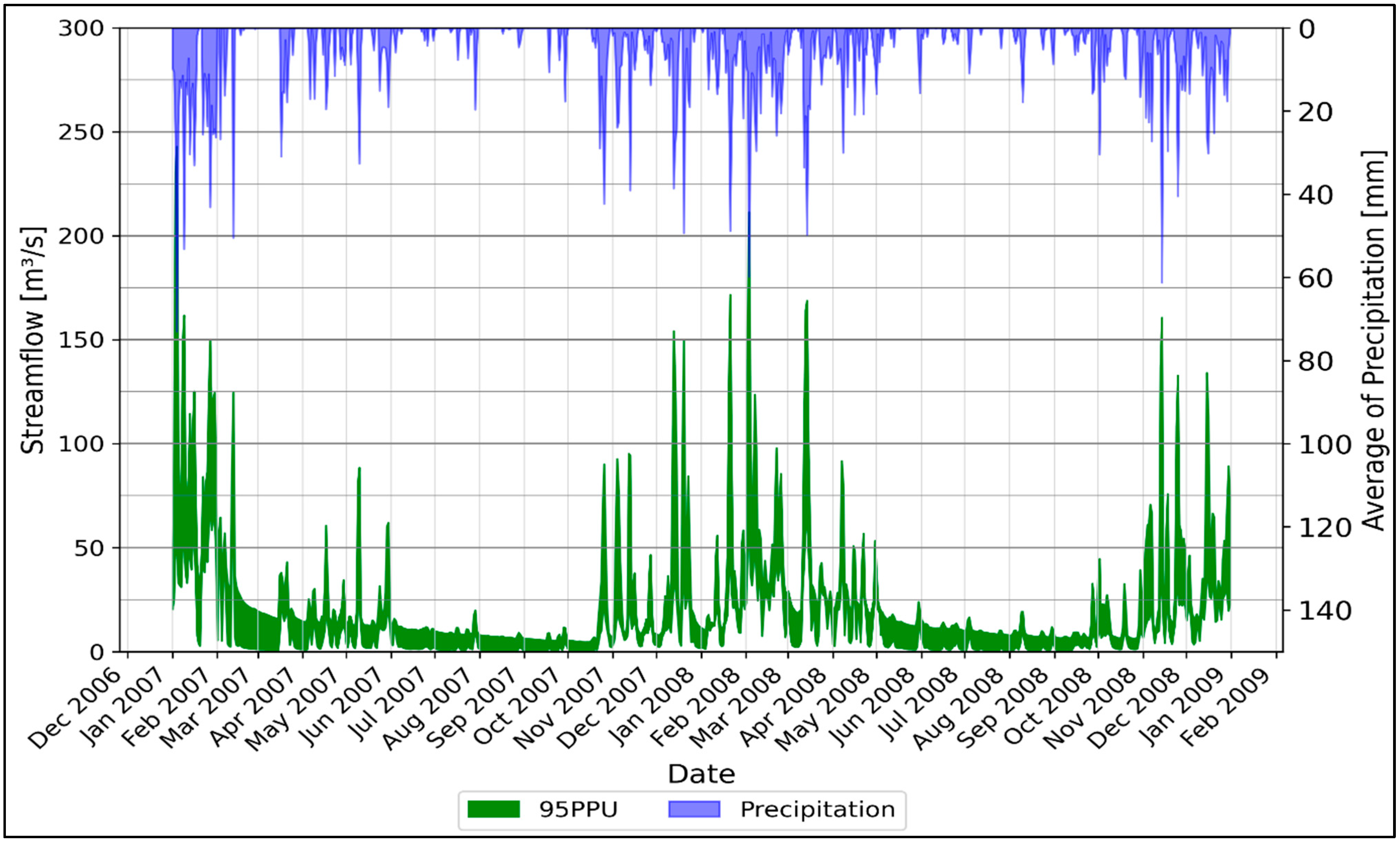
The 95PPU analysis (Figure 13) shows that uncertainty is strongly conditioned by the lowest ${ K}_{sat}$ value tested. When the full range (10.019–1001.931 cm day⁻¹) is considered, the mean uncertainty bandwidth for the full period reaches 12.91 m³ s⁻¹ ($CV = 164.52\%$). Seasonal values follow the same structure, with mean bandwidths of 20.81 m³ s⁻¹ in the wet season ($CV = 128.91\%$) and 5.03 m³ s⁻¹ in the dry season ($CV = 153.62\%$). However, this elevated dispersion is primarily associated with the inclusion of the lowest conductivity scenario (S31).

When S31 is excluded and the analysis is restricted to 70.135–1001.931 cm day⁻¹ (Figure 14), the mean bandwidth for the full period decreases to 5.59 m³ s⁻¹, representing a reduction of approximately 57%. Similar reductions occur seasonally, with wet-season bandwidth decreasing from 20.81 to 9.50 m³ s⁻¹ and dry-season ${\mu }_{Bandwidth}$ from 5.03 to 1.69 m³ s⁻¹. Although coefficients of variation remain high (full period $CV = 186.78\%$; wet = 141.34%; dry = 163.23%), the substantial reduction in absolute bandwidth demonstrates that the majority of predictive spread is driven by extremely low ${ K}_{sat}$ values.

These results indicate that uncertainty amplification is concentrated near the lower bound of the parameter space. Once ${ K}_{sat}$ exceeds approximately 70 cm day⁻¹, both performance metrics (Table 10; Figure 12) and uncertainty magnitudes stabilize, and additional increases in conductivity produce comparatively limited changes in either efficiency or predictive dispersion. Collectively, the evidence supports threshold-controlled behavior in which ${ K}_{sat}$ exerts strong influence under low-conductivity conditions, while operating within a regime of diminishing marginal impact across intermediate and high values.

3.2. Soil-Focused Calibration Strategy

The baseline configuration (S40), representing uniform ±10% variation in VGM parameters, produced $NSE$ = 0.50 and $PBIAS$ = 25.32%, indicating moderate predictive skill with substantial positive bias. All subsequent analyses are interpreted relative to this reference (

Table 11. Calibration over the 2-year simulation period (2008–2009).

SIM	Parameter Calibrated	$\mathit{P}\mathit{B}\mathit{I}\mathit{A}\mathit{S}$	$\mathit{N}\mathit{S}\mathit{E}$
S40	Calibration baseline (10% VGM variation)	25.32	0.50
S41	${\theta }_s\left(+20\mathrm{\%}\right)$	22.34	0.57
S42	${\theta }_s\left(+30\mathrm{\%}\right)$	18.93	0.61
S43	$n(+20\mathrm{\%})$	22.14	0.59
S44	${\theta }_s\left(+20\mathrm{\%}\right)$, $n(+20\mathrm{\%})$	18.41	0.61
S45	${\theta }_s\left(+30\mathrm{\%}\right)$, $n(+20\mathrm{\%})$	14.43	0.60
S46	$n(+30\mathrm{\%})$	20.54	0.61
S47	${\theta }_s\left(+20\mathrm{\%}\right)$, $n(+30\mathrm{\%})$	16.52	0.60
S48	${\theta }_s\left(+30\mathrm{\%}\right)$, $n(+30\mathrm{\%})$	12.27	0.57
S49	$n(+50\mathrm{\%})$	19.87	0.60
S50	${\theta }_s\left(+20\mathrm{\%}\right)$, $n(+50\mathrm{\%})$	15.78	0.57
S51	${\theta }_s\left(+30\mathrm{\%}\right)$, $n(+50\mathrm{\%})$	11.24	0.53
S52	${\theta }_s\left(+20\mathrm{\%}\right)$, $KF=15$	21.65	0.56
S53	${\theta }_s\left(+30\mathrm{\%}\right)$, $KF=15$	18.64	0.60
S54	$n(+20\mathrm{\%})$, $KF=15$	21.80	0.58
S55	${\theta }_s\left(+20\mathrm{\%}\right)$, $n(+20\mathrm{\%}),KF=15$	18.56	0.60
S56	${\theta }_s\left(+30\mathrm{\%}\right)$, $n(+20\mathrm{\%}),KF=15$	15.03	0.60
S57	$n(+30\mathrm{\%})$, $KF=15$	20.69	0.59
S58	${\theta }_s\left(+20\mathrm{\%}\right)$, $n(+30\mathrm{\%}),KF=15$	17.18	0.59
S59	${\theta }_s\left(+30\mathrm{\%}\right)$, $n(+30\mathrm{\%}),KF=15$	13.38	0.57
S60	$n(+50\mathrm{\%})$, $KF=15$	20.29	0.58
S61	${\theta }_s\left(+20\mathrm{\%}\right)$, $n(+50\mathrm{\%}),KF=15$	16.68	0.57
S62	${\theta }_s\left(+30\mathrm{\%}\right)$, $n(+50\mathrm{\%}),KF=15$	12.85	0.54
S63	${\theta }_s\left(+30\mathrm{\%}\right)$, ${\theta }_r\left(-30\mathrm{\%}\right),$ $\alpha \left(-70\mathrm{\%}\right)$, $n\left(+50\mathrm{\%}\right)$, $K_{sat}\left(+100\mathrm{\%}\right)$	3.88	0.45

).

Increasing ${\theta }_s$ generated a clear and monotonic improvement in model performance. A +20% increment (S41) increased $NSE$ from 0.50 to 0.57 (+0.07) and reduced $PBIAS$ to 22.34% (−2.98 percentage points). Expanding the increment to +30% (S42) further increased $NSE$ to 0.61 (+0.11 relative to baseline) and reduced $PBIAS$ to 18.93%, corresponding to a 6.39 percentage-point reduction (approximately 25% relative decrease in bias). The marginal gain between +20% and +30% ${\theta }_s$ was therefore +0.04 in $NSE$ and −3.41 percentage points in $PBIAS$, indicating continued but reduced incremental benefit beyond +20%.

Adjustments in n produced a similar efficiency response but with weaker bias control. Increasing $n$ by +20% (S43) raised $NSE$ to 0.59 (+0.09) while reducing $PBIAS$ to 22.14% (−3.18). At +30% (S46), $NSE$ reached 0.61 (+0.11), matching the maximum obtained with ${\theta }_s$, although $PBIAS$ remained slightly above the acceptable 20% threshold (20.54%). Further increasing n to +50% (S49) did not yield additional efficiency gains ($NSE$ = 0.60) but reduced bias to 19.87%. The reduction in $NSE$ from 0.61 to 0.60 between +30% and +50% $n$ indicates performance saturation beyond moderate increments, despite continued bias reduction.

Combined perturbations of ${\theta }_s$ and $n$ revealed non-additive interaction effects. The configuration ${\theta }_s$ + 20% and $n$ + 20% (S44) produced $NSE$ = 0.61 and $PBIAS$ = 18.41%, satisfying both performance thresholds. Increasing ${\theta }_s$ to +30% while maintaining $n$ at +20% (S45) yielded $NSE$ = 0.60 and $PBIAS$ = 14.43%, representing a 10.89 percentage-point reduction relative to baseline (approximately 43% bias reduction). However, further escalation to ${\theta }_s$ + 30% and $n$ + 30% (S48) reduced $NSE$ to 0.57, and combining ${\theta }_s$ + 30% with $n$ + 50% (S51) decreased $NSE$ further to 0.53, despite lowering $PBIAS$ to 11.24%. These results demonstrate that while moderate simultaneous increases improve both efficiency and bias, larger combined perturbations degrade hydrograph dynamics, indicating diminishing and eventually negative marginal returns.

Simulations incorporating increased horizontal conductivity ($KF=15$; S52–S62) did not produce systematic improvements relative to their $KF=10$ counterparts. In all comparable configurations, $NSE$ either remained unchanged or decreased by 0.01–0.02. For example, S42 ($KF=10$) achieved $NSE$ = 0.61, whereas its $KF=15$ counterpart (S53) produced $NSE$ = 0.60. Similarly, S44 (0.61) decreased to 0.60 in S55. Bias reductions were also comparable but not superior under $KF=15$. These results indicate that increasing horizontal conductivity does not significantly enhance predictive performance under the tested conditions.

The aggregated configuration (S63), which combined all individually favorable adjustments (${\theta }_s$ + 30%, ${\theta }_r$− 30%,$\alpha$ − 70%, $n$ + 50%, ${ K}_{sat}$+ 100%), produced the lowest bias ($PBIAS$ = 3.88%, an 84.7% reduction relative to baseline) but simultaneously reduced $NSE$ to 0.45, below the baseline value. This outcome demonstrates that aggressive multi-parameter adjustments can minimize volume error while degrading temporal dynamics, evidencing structural compensation effects.

Among all tested configurations, S45 (${\theta }_s$+ 30%, $n$ + 20%) provides the most balanced trade-off between efficiency and bias. Although its $NSE$ (0.60) is marginally lower than the maximum observed value (0.61 in S42, S44, and S46), the difference of 0.01 units represents less than a 2% relative reduction in efficiency. In contrast, $PBIAS$ decreases to 14.43%, corresponding to a 10.89 percentage-point reduction relative to the baseline (25.32%) and a 4.50 percentage-point improvement compared to S42 (18.93%), which achieved the same maximum $NSE$. This configuration therefore achieves a 43% relative reduction in bias while maintaining efficiency at the performance plateau (~0.60–0.61).

Configurations with higher $n$ increments (e.g., S48 and S51) further reduced bias to 12.27% and 11.24%, respectively, but at the expense of a substantial $NSE$ decline (0.57 and 0.53), indicating degradation of hydrograph dynamics. Conversely, configurations maximizing $NSE$ (0.61) without a simultaneous ${\theta }_s$ increase (e.g., S46) failed to reduce bias below the 20% threshold.

Therefore, S45 represents the optimal compromise between volumetric accuracy and temporal dynamics, minimizing systematic overestimation while preserving efficiency near its maximum attainable level. This result indicates that moderate structural enhancement of soil ${\theta }_s$ combined with $n$ yields the most hydrologically consistent calibration outcome.

3.3. Validation of the Soil-Focused Calibration Strategy

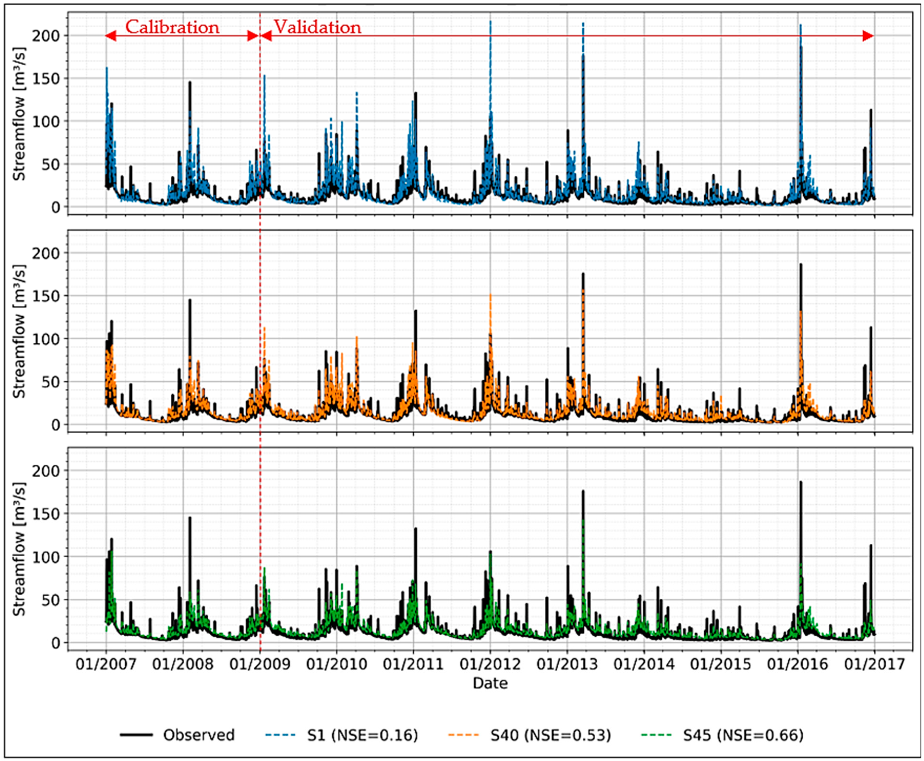
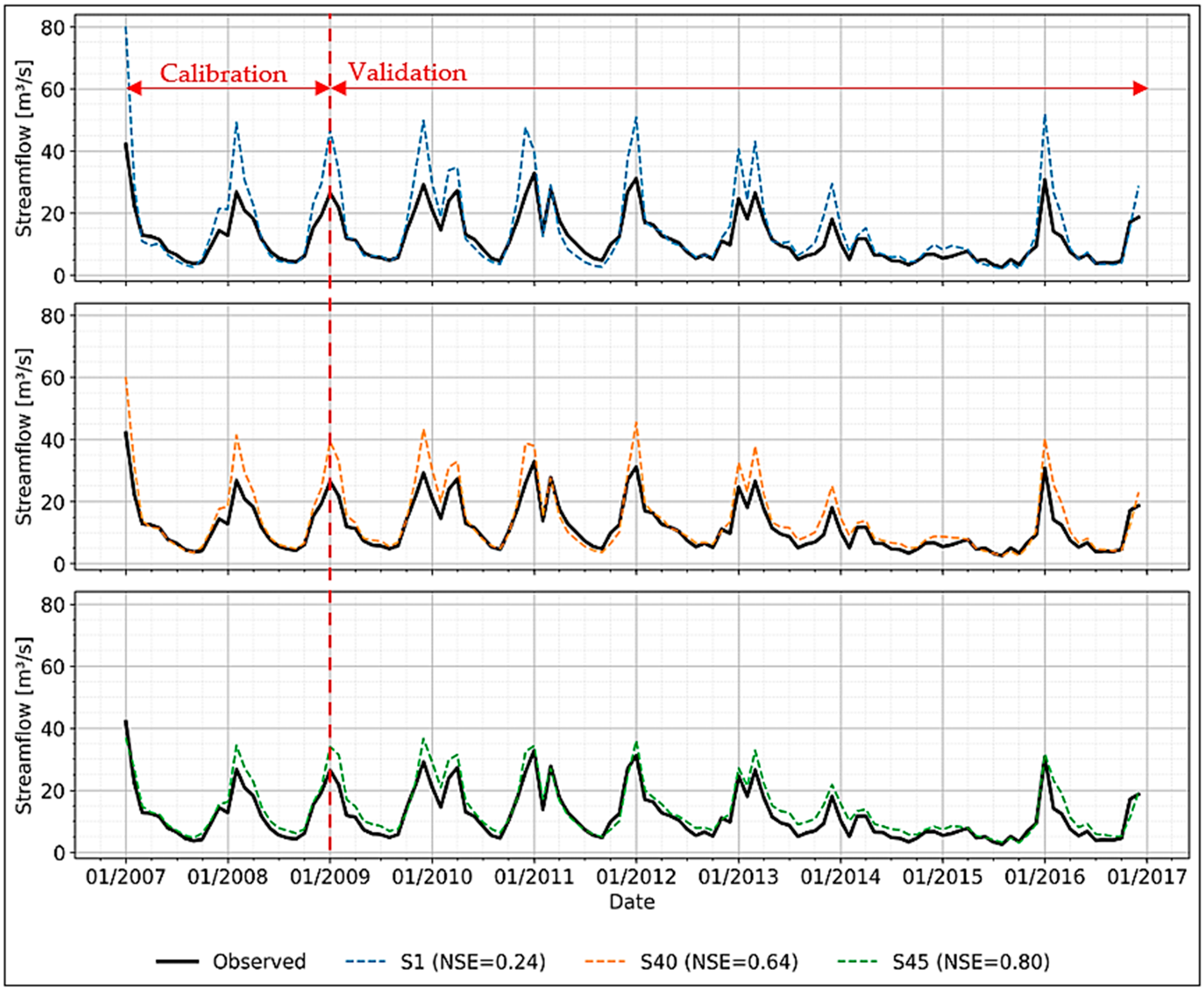
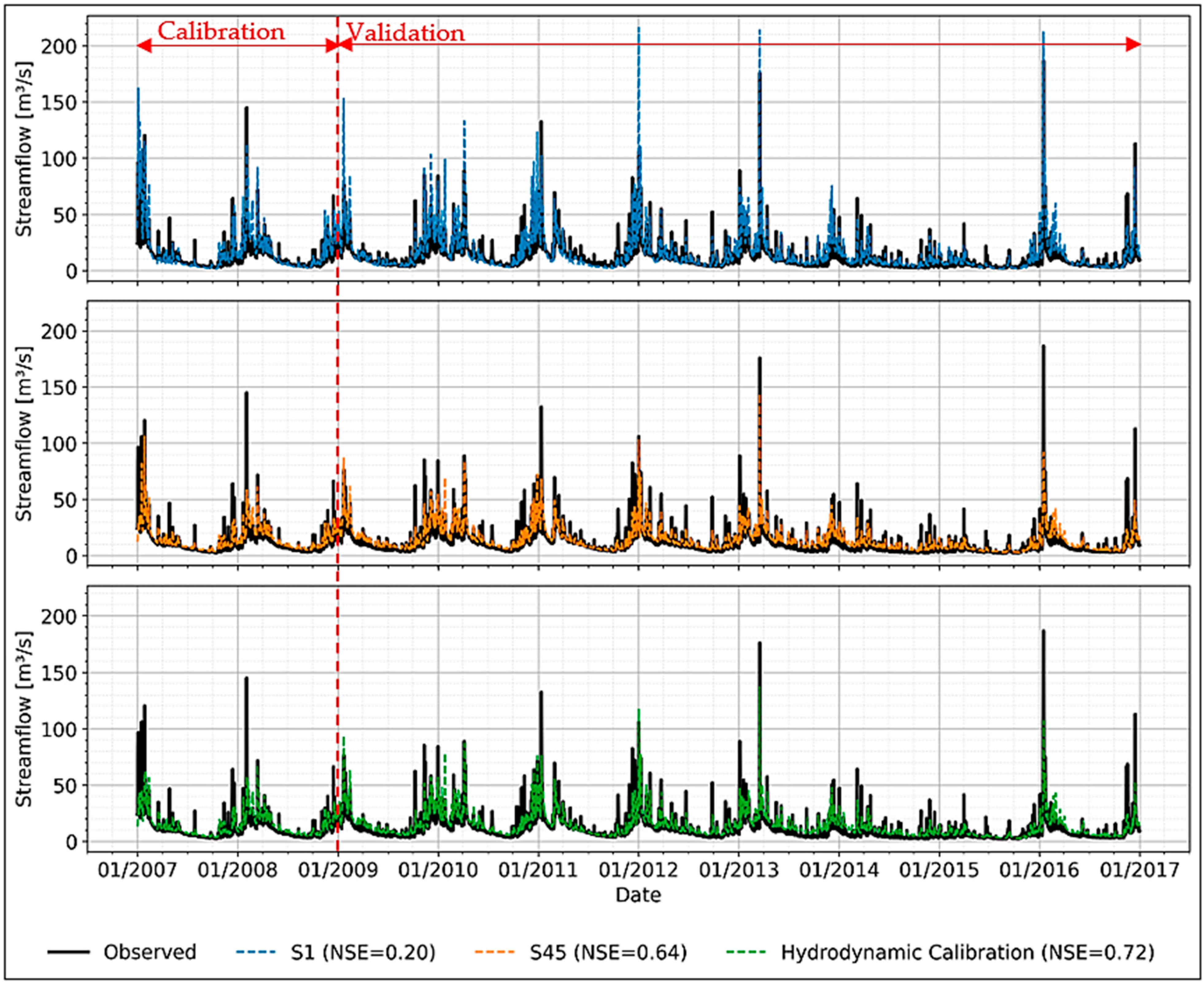
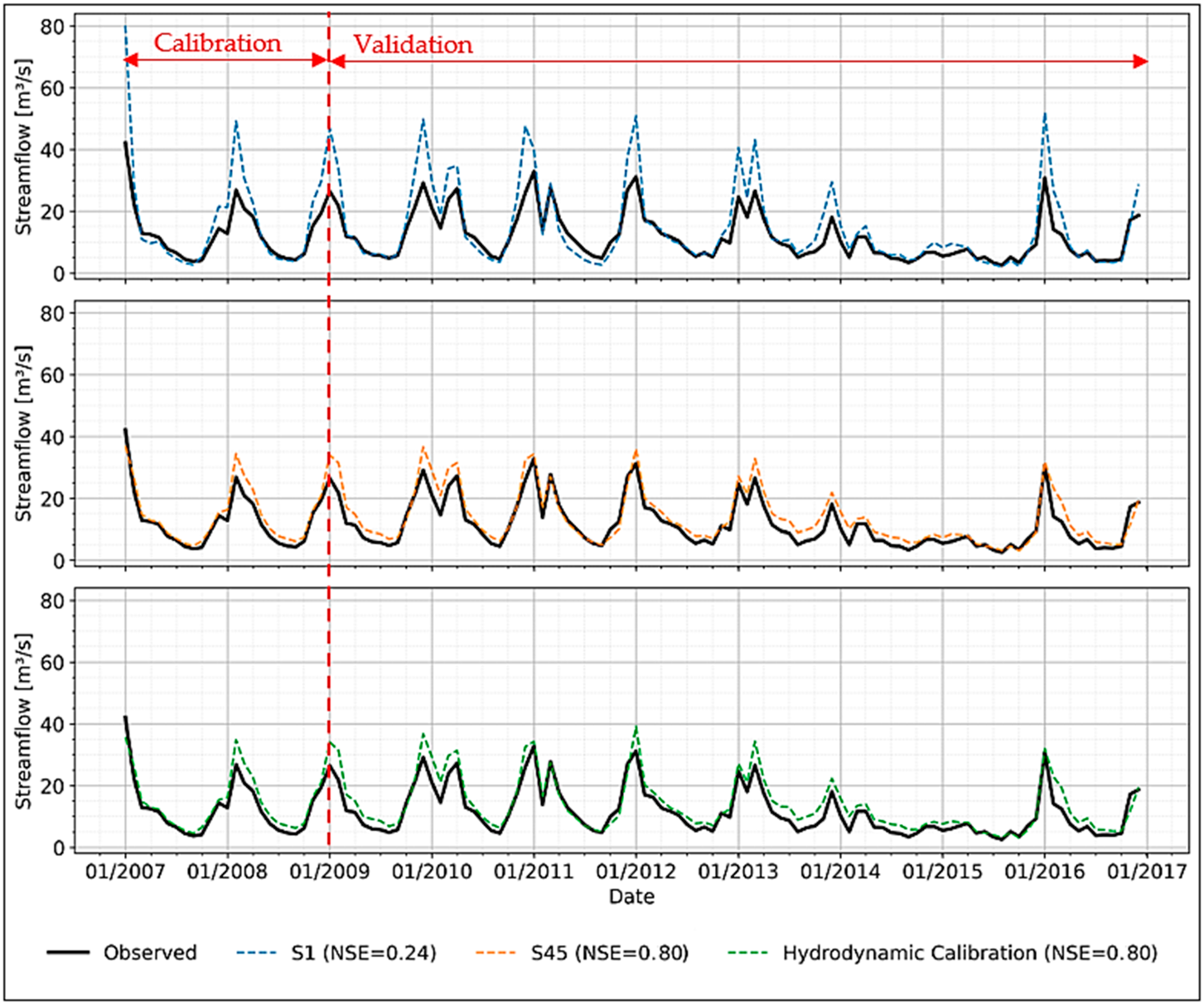
The eight-year validation period (2009–2016) confirms the robustness and temporal transferability of the calibrated soil parameterization derived in Section 3.2. Scenario S45 consistently outperformed both the uncalibrated reference (S1) and the partially calibrated baseline (S40) across full-period and seasonal evaluations (

Table 12. Daily streamflow performance throughout the 8-year validation period (2009–2016).

SIM		$\mathit{N}\mathit{S}\mathit{E}$			$\mathit{P}\mathit{B}\mathit{I}\mathit{A}\mathit{S}$
	Full Period	Wet Season	Dry Season	Full Period	Wet Season	Dry Season
S1	0.20	0.02	0.57	25.69	39.99	−2.14
S40	0.53	0.45	0.66	20.95	26.44	10.26
S45	0.66	0.62	0.65	19.55	16.55	24.36

).

On the daily scale, S45 increased $NSE$ from 0.20 (S1) to 0.66, representing an absolute gain of 0.46 units and a relative improvement of 230% in predictive efficiency. Compared to S40 ($NSE$ = 0.53), S45 achieved an additional gain of 0.13 units (+25%), confirming that targeted calibration of ${\theta }_s$ and $n$ yields improvements beyond uniform parameter perturbation.

Bias reduction was also substantial relative to S1. Full-period $PBIAS$ decreased from 25.69% (S1) to 19.55% (S45), corresponding to a 6.14 percentage-point reduction. Although the improvement over S40 (20.95%) was moderate (−1.40 percentage points), efficiency gains were markedly higher, indicating that S45 primarily enhanced hydrograph dynamics rather than merely correcting volumetric bias.

Seasonal diagnostics reveal distinct improvements in high-flow conditions. During the wet season, $NSE$ increased from 0.02 (S1) to 0.62 (S45), an absolute gain of 0.60 units. This represents the largest seasonal improvement and confirms that calibration substantially enhanced peak-flow simulation. Wet-season $PBIAS$ was reduced from 39.99% (S1) to 16.55% (S45), corresponding to a 23.44 percentage-point reduction (≈59% relative decrease), demonstrating strong correction of systematic overestimation under high-discharge conditions.

Dry-season performance exhibited a different response. While $NSE$ improved from 0.57 (S1) to 0.65 (S45), bias shifted from slight underestimation (−2.14%) to overestimation (24.36%). Compared to S40 ($PBIAS$ = 10.26%), S45 increased dry-season bias by 14.10 percentage points. This indicates that calibration prioritized dynamic fidelity during high-flow periods at the expense of low-flow volumetric accuracy. Nevertheless, dry-season $NSE$ remained high (0.65), indicating preservation of temporal variability despite increased bias.

Hydrograph comparisons (Figure 15) corroborate these quantitative metrics. S1 systematically exaggerated flood peaks and displayed delayed recession behavior. S40 reduced peak magnitude but retained event-scale discrepancies. S45 produced the closest alignment with observed discharge, particularly during major storm events, with improved peak timing and recession slope representation. The progressive contraction of peak residuals from S1 to S45 is consistent with the substantial wet-season $NSE$ increase observed numerically.

On the monthly scale (Figure 16), S45 achieved $NSE$ = 0.80, representing a 0.27-unit increase over S40 and a 0.60-unit increase over S1. This substantial gain indicates that calibration effects propagate across temporal aggregation levels and that parameter adjustments improve not only event-scale dynamics but also cumulative water balance representation.

Flow duration curves (Figure 17) further highlight performance gains across discharge quantiles. S1 overestimated high flows (low exceedance probabilities) and underestimated mid-range flows. S40 reduced high-flow deviations but maintained discrepancies in intermediate percentiles. S45 achieved the closest agreement across the full exceedance spectrum, particularly between the 10–40% probability range, indicating improved representation of frequent storm-driven discharges while preserving baseflow structure.

Collectively, validation results demonstrate that calibration of ${\theta }_s$ and $n$ improves predictive consistency across multiple diagnostic dimensions: daily dynamics (+0.46 $NSE$ full period), wet-season flood representation (+0.60 $NSE$), monthly aggregation (+0.60 $NSE$ relative to S1), and frequency-based discharge distribution. Performance gains are most pronounced under high-flow conditions, confirming that soil water storage capacity and pore-size distribution exert dominant control on runoff generation dynamics during intense precipitation events. While some dry-season bias amplification occurs, overall efficiency gains and improved hydrograph structure indicate that S45 provides the most hydrologically coherent and transferable configuration across temporal scales.

3.4. Improving Streamflow Simulation by Incorporating Hydrodynamic Parameters

After soil-focused calibration (Setup S45), hydrodynamic parameters were adjusted to evaluate their incremental contribution to model performance.

Table 13. Model performance ($NSE$) for monthly and daily time scales during the hydrodynamic calibration and validation periods.

SIM	Daily		Monthly
	Calibration	Validation	Calibration	Validation
S1 (reference)	0.01	0.20	−0.30	0.24
S45 (soil calibration)	0.60	0.66	0.86	0.80
Hydrodynamic Calibration	0.63	0.72	0.87	0.80

summarizes daily and monthly $NSE$ values for the calibration and validation periods.

During validation (2009–2016), daily $NSE$ increased from 0.66 (S45) to 0.72 after hydrodynamic refinement, corresponding to an absolute gain of 0.06 units (+9.1% relative improvement). In contrast, monthly validation $NSE$ remained unchanged at 0.80.

During calibration, daily $NSE$ increased from 0.60 (S45) to 0.63 (+0.03), while monthly $NSE$ increased marginally from 0.86 to 0.87 (+0.01). The larger improvement observed during validation compared to calibration suggests enhanced generalization rather than overfitting.

When compared to the reference simulation (S1), total validation improvement in daily $NSE$ reached +0.52 units (0.20 → 0.72). Of this total gain:

• Soil calibration (S1 → S45) contributed +0.46 units (88% of total improvement);
• Hydrodynamic calibration (S45 → Hydro) contributed +0.06 units (12% of total improvement).

For monthly validation performance, soil calibration alone increased $NSE$ by +0.56 units (0.24 → 0.80), while hydrodynamic refinement produced no additional improvement.

These results quantitatively demonstrate that soil hydraulic calibration controls the dominant share of performance enhancement, whereas hydrodynamic parameters provide secondary refinement restricted primarily to daily dynamics.

Daily hydrograph comparison (Figure 18) shows a progressive reduction in peak overestimation from S1 to S45 and further attenuation after hydrodynamic adjustment. Peak discharge residuals decrease systematically, and recession curves exhibit improved slope consistency. Event-scale variability is more accurately reproduced after routing refinement, particularly during high-intensity rainfall events.

Monthly hydrographs (Figure 19) display minimal visible differences between S45 and the hydrodynamically refined setup, confirming the absence of additional aggregated-scale performance gains.

4. Discussion

4.1. Relative Importance of VGM Parameters

The sensitivity analysis indicates differentiated levels of influence among the VGM parameters within the tested ranges. Based strictly on the magnitude and structure of performance variation observed in Section 3.1 (Table 6, Table 7, Table 8, Table 9 and Table 10), the parameters can be organized as follows: ${\theta }_s$ and $n$ (higher influence), ${ K}_{sat}$ (threshold-dependent influence), and ${\theta }_r$ and $\alpha$ (lower influence). This hierarchy aligns with previous findings in distributed hydrological modeling, where soil water retention and pore-size distribution parameters often exert stronger control on discharge simulations than residual water content parameters [54,55].

At the top of this hierarchy, ${\theta }_s$ emerges as the most influential parameter within the evaluated configuration. Its variation produces strong, coherent, and nearly linear improvements in performance metrics across the tested range. This dominant role is consistent with previous findings emphasizing saturated water content as a primary regulator of runoff generation processes in MOHID-Land and other VGM-based models [19].

Physically, ${\theta }_s$ defines effective porosity and maximum transient storage within the van Genuchten formulation [8], directly controlling the volumetric boundary of the soil reservoir. The near-linear response observed here indicates that increases in storage capacity proportionally enhance the model’s ability to attenuate peak flows [56]. Unlike parameters exhibiting internal optima, no intrinsic asymptotic behavior was detected within the evaluated ${\theta }_s$ range. The only limitation is pedological realism: ${\theta }_s$ is bounded by soil porosity.

The amplified wet-season sensitivity aligns with previous studies reporting stronger parameter effects under saturation-controlled hydrological regimes [57]. Moreover, the calibrated ${\theta }_s$ range is coherent with the high forest cover (>60%) of the catchment, where enhanced macroporosity and structural connectivity are expected [58,59]. These findings suggest a closer alignment between modeled storage behavior and observed discharge dynamics, although interactions between parameters may influence model behavior.

Closely following ${\theta }_s$, $n$ also functions as a dominant control parameter, though through redistribution dynamics rather than volumetric storage. This finding aligns with earlier MOHID-Land simulations identifying $n$ as one of the most influential VGM parameters [19,20]. Similarly, Li et al. [60] demonstrated the strong influence of $n$ on soil hydraulic behavior, and Bindas et al. [61] reported improvements in routing efficiency following calibration of hydraulic shape parameters.

Unlike ${\theta }_s,$ however, $n$ exhibits a structurally bounded response. Performance improves markedly up to an optimal range but stabilizes beyond it, indicating a bounded response with an identifiable optimal range within the tested interval. This suggests that once the retention curve adequately represents pore-size distribution, further steepening does not substantially modify runoff partitioning. Thus, whereas ${\theta }_s$ governs storage magnitude, $n$ governs drainage kinetics and hydrograph format.

Below these primary controls, ${ K}_{sat}$ occupies an intermediate position. Its threshold-dominated behavior aligns with previous studies highlighting the sensitivity of runoff generation to low hydraulic conductivity zones. Jin et al. [62] reported that unrealistically low ${ K}_{sat}$ values substantially increase surface runoff, while higher values yield diminishing performance improvements. Similarly, Hu et al. [63] emphasized the role of hydraulic conductivity in controlling infiltration–runoff partitioning.

The present results confirm that ${ K}_{sat}$ primarily governs infiltration limitation rather than continuously controlling hydrograph dynamics. Once a functional conductivity threshold is exceeded, runoff responses become increasingly regulated by soil storage and retention characteristics rather than by conductivity magnitude itself. This pattern is consistent with a shift toward storage-dominated runoff regulation, as also reported in previous studies investigating infiltration–runoff partitioning under varying hydraulic conductivity conditions [62,63]. At the lower end of the hierarchy, ${\theta }_r$ demonstrates limited hydrological leverage, consistent with previous findings identifying it as a minor contributor to streamflow simulation in VGM-based models [19]. Conceptually, higher ${\theta }_r$ values increase immobile water storage and restrict gravitational drainage, as described by Du et al. [64] and Bear et al. [65].

The present analysis confirms that reducing ${\theta }_r$ slightly enhances drainable porosity and subsurface connectivity but does not substantially alter catchment-scale discharge dynamics. Its influence remained limited within the tested range and modeling configuration.

Finally, $\alpha$ exhibits the weakest and least stable sensitivity pattern. Sales et al. [19] similarly reported limited overall influence of $\alpha$ across simulation periods. Because α modifies the air-entry pressure and the curvature of the retention curve rather than storage magnitude itself, its impact on streamflow remains indirect and regime-dependent. The absence of directional consistency in its response further supports its classification as a secondary parameter within the VGM hierarchy.

In summary, the narrative of parameter importance is coherent and progressively structured:

• ${\theta }_s$—monotonic and high-magnitude improvement within the tested range.
• $n$—high-magnitude but non-linear response with an internal optimum.
• $K_{sat}$—threshold-controlled influence with strong effects at low values and plateau behavior thereafter.
• ${\theta }_r$ and $\alpha$—low-magnitude, approximately linear or regime-dependent responses without strong structural leverage.

This ordered hierarchy has direct implications for calibration strategy, indicating that optimization efforts should prioritize ${\theta }_s$ and $n$ before refining ${ K}_{sat}$, while ${\theta }_r$ and $\alpha$ require only constrained adjustments within physically plausible bounds.

4.2. Dominance Seasonal Trade-Off and Process Interpretation

While Section 4.1 established the relative hierarchy of VGM parameters, the seasonal analysis reveals a deeper process-based differentiation: parameter influence is not static but is activated according to dominant hydrological regimes [64]. The wet and dry seasons represent distinct control states of the soil system, and the observed sensitivities reflect shifts between storage-driven and redistribution-driven dynamics rather than a simple amplification of magnitude [66].

During the wet season, system behavior is governed by proximity to saturation. Under these conditions, runoff generation becomes highly responsive to parameters that regulate effective storage and hydraulic connectivity [67]. The strong seasonal amplification observed for ${\theta }_s$ indicates that peak-flow dynamics are primarily controlled by the volumetric limits of transient soil storage [56,68]. This reflects a structural condition in which incremental changes in storage capacity directly modify the threshold for saturation-excess activation. In such regimes, performance improvements are linked to attenuation capacity rather than flow timing adjustments.

In contrast, dry-season dynamics expose a different control structure. Here, the system operates far from saturation, and discharge becomes increasingly dependent on redistribution efficiency and drainage persistence [55,58]. The seasonal trade-off associated with $n$ illustrates this shift clearly. Parameter values that enhance wet-season performance by accelerating drainage and sharpening hydraulic gradients may simultaneously reduce the soil moisture retention required to sustain baseflow. This reveals a kinetic–storage tension: improving responsiveness under high-moisture conditions can destabilize low-flow representation when redistribution becomes excessive [19]. The existence of a bounded optimal range for n therefore reflects a regime-dependent balance rather than simple parameter sensitivity [51].

The analysis of dry-season dynamics demonstrates that parameter refinement progressively reduced low-flow underestimation, suggesting an improved representation of subsurface drainage persistence without altering peak-flow magnitude. This performance gain suggests that adjusting retention and conductivity parameters effectively suggests improved simulation of recession dynamics and delayed drainage responses. Physically, moderate retention values may marginally contribute to sustaining soil moisture availability during recession periods and, consequently, to delayed flow release [69], which is essential for sustaining discharge during the dry months.

${ K}_{sat}$ exhibits yet another seasonal pattern. Its influence concentrates under conditions where infiltration capacity constrains runoff generation [62]. However, once infiltration exceeds rainfall intensity and surface limitation is removed, seasonal differentiation diminishes [63]. The transition observed in Section 3 indicates that conductivity primarily determines whether the system operates under infiltration-limited or storage-controlled behavior. After that transition, further increases in ${ K}_{sat}$ do not significantly alter seasonal discharge structure. Unlike $n$, conductivity does not create opposing seasonal objectives but instead governs entry into a hydraulically feasible regime.

By contrast, ${\theta }_r$ and $\alpha$ display weak seasonal modulation. Their effects do not intensify under either hydrological extreme, suggesting that parameters governing residual moisture and air-entry scaling play a limited role in controlling integrated discharge dynamics under the climatic conditions examined [49,60]. Their influence appears subordinate to parameters directly involved in storage magnitude and drainage kinetics.

Taken together, the seasonal behavior of the parameters reveals that hydrological calibration cannot be reduced to identifying the most sensitive parameter in aggregate metrics. Instead, the results demonstrate that model performance emerges from the balance between storage expansion, redistribution rate, and infiltration capacity across contrasting moisture regimes. Trade-offs arise when improvements under one regime amplify structural imbalances under another. This regime-dependent activation of soil hydraulic controls underscores the need for seasonally aware calibration strategies, particularly in basins where rapid response and pronounced wet–dry contrasts coexist [69].

This regime-dependent behavior is consistent with previous studies highlighting the importance of seasonal dynamics in controlling parameter sensitivity in hydrological models [19,20,66,70].

4.3. Implications for Deterministic Soil-Focused Calibration

The hierarchical behavior identified among the VGM parameters has direct methodological implications for deterministic soil-focused calibration. Rather than assuming equal contribution of soil hydraulic parameters to model adjustment, the results indicate that each parameter plays a distinct structural role within the hydrological system. This interpretation aligns with physically based modeling perspectives that emphasize structural parameter dominance over purely statistical optimization approaches [54].

The comparative scenario analysis demonstrated that adjustments affecting storage architecture exert the strongest systemic influence. In particular, ${\theta }_s$ directly regulates maximum soil water storage capacity and therefore modifies runoff partitioning at its source. Storage-controlled dynamics have long been recognized as fundamental determinants of catchment response [71], providing conceptual support for prioritizing storage-related parameters in calibration routines. Moreover, incremental modifications of ${\theta }_s$ tend to produce proportionate hydrological responses, which is consistent with theoretical expectations regarding stable objective-function gradients for structurally dominant parameters [72].

Following storage alignment, redistribution dynamics become the next relevant control. Parameter $n$ governs the steepness and shape of the soil water retention curve, thereby influencing subsurface flow redistribution [8,19,20]. However, unlike ${\theta }_s$, $n$ introduces nonlinear response behavior associated with pore-size distribution effects. Previous soil hydraulic sensitivity studies (e.g., Schaap & Leij [73]) have shown that retention-curve shape parameters may introduce additional calibration complexity when insufficiently constrained. Thus, while n exerts strong systemic control, its calibration requires physically informed boundaries to avoid disproportionate subsurface distortions.

In contrast, ${ K}_{sat}$ primarily operates as a hydraulic threshold parameter. Its functional role is to prevent artificial infiltration limitation once conductivity exceeds rainfall intensity, consistent with infiltration theory [19]. Beyond this functional threshold, further refinement of ${ K}_{sat}$ produces limited structural alteration of hydrograph form. Although previous work demonstrated incremental gains from ${ K}_{sat}$ adjustment under fixed retention conditions [20], the present results show that its influence becomes conditional once ${\theta }_s$ and $n$ are recalibrated.

At the lower end of the dominance hierarchy, ${\theta }_r$ and $\alpha$ exhibit constrained structural impact. Their effects are often intertwined with higher-order retention parameters, and attempts to correct hydrograph deficiencies through these variables may introduce compensatory distortions without resolving underlying storage or redistribution imbalances. This behavior is consistent with the equifinality framework described by Beven [54], wherein secondary parameters can mask structural inconsistencies without structurally improving model realism.

Importantly, the hierarchical calibration pattern observed here emerged empirically from comparative scenario testing rather than from a predefined algorithmic sequence. The results therefore support, rather than presuppose, a structured soil-focused calibration strategy in which:

• A moderate global adjustment improves baseline structural consistency.
• Targeted recalibration of ${\theta }_s$ and $n$ is responsible for most of the efficiency gains.
• Additional parameter tuning yields diminishing returns and may not justify increased calibration complexity.

Within the tested parameter space and hydropedological context, this evidence indicates that concentrated recalibration of dominant soil retention properties constitutes the most efficient strategy for enhancing watershed-scale streamflow simulation.

4.4. Calibration Efficiency and Structural Performance

The combined calibration and validation results demonstrate that model efficiency reflects structural coherence within the soil hydraulic framework rather than simple parameter maximization. Although multiple configurations achieved acceptable performance during the calibration phase, only moderate and coordinated adjustments of the dominant retention parameters sustained efficiency under long-term validation. This reinforces the hierarchical behavior discussed in Section 4.3 and confirms that structural alignment, rather than cumulative parameter amplification, governs predictive robustness.

The progressive improvement from the baseline configuration to the targeted retention-parameter scenarios indicates that enhancing soil water storage capacity and retention-curve steepness improves hydrological partitioning in a structurally consistent manner. The validation diagnostics, including hydrograph agreement, seasonal performance, monthly aggregation classified as “very good” according to Moriasi et al. [53], and flow duration curve coherence, collectively demonstrate that recalibration of ${\theta }_s$ and $n$ restores balance among infiltration, storage, percolation, and runoff generation processes. These improvements align with hydropedological interpretations emphasizing the unsaturated zone as a structural mediator of precipitation–runoff interactions [66,74].

In contrast, excessive increases in retention parameters or aggregated amplification of multiple variables produced diminishing or negative efficiency gains. The aggregated scenario (S63) provides clear evidence that parameter optimality is not additive in nonlinear hydrological systems. Although bias reduction was achieved, overall efficiency deteriorated, illustrating interaction effects consistent with nonlinear parameter behavior and equifinality dynamics [54]. This confirms that combining individually favorable parameter adjustments does not guarantee structural improvement.

A comparable interaction pattern is observed for the $KF$. Previous work demonstrated that increasing horizontal conductivity enhanced model performance when calibrated independently under fixed retention conditions [34]. However, once ${\theta }_s$ and $n$ were recalibrated, additional increases in $KF$ frequently failed to yield further gains. This inversion indicates conditional rather than global optimality of conductivity adjustments and highlights the nonlinear coupling between hydraulic conductivity and retention structure within the VGM formulation [16,17].

Importantly, these findings consolidate the empirical hierarchy established earlier. Calibration efficiency emerges from coordinated adjustment of dominant retention properties, whereas secondary parameters primarily ensure hydraulic consistency within physically plausible bounds. Moderate recalibration of ${\theta }_s$ and $n$ enhances predictive stability across temporal scales, while cumulative parameter amplification introduces structural imbalance and diminishing returns.

Within the tested parameter space and hydropedological context, the most robust performance was achieved not by maximizing individual parameters but by restoring hydraulic architecture through balanced retention recalibration. Calibration efficiency therefore reflects structural parameter interaction rather than numerical extremization, reinforcing the soil-focused dominance-based logic derived from the comparative scenario analysis.

This structural reliability has broader implications for watershed management applications. Accurate representation of soil retention properties is essential when evaluating interventions designed to modify infiltration and subsurface storage, including nature-based solutions aimed at enhancing water availability. As discussed by Silva Junior et al. [75], strategies that promote infiltration and soil–water retention can play a critical role in mitigating water scarcity. Physically consistent soil parameterization therefore becomes a prerequisite for credible scenario-based assessments of such interventions.

Moreover, the identification of dominant soil hydraulic parameters provides a structured pathway for incorporating spatially distributed datasets into future model refinement. Remote sensing products, such as long-term surface water and vegetation indicators analyzed by Costa et al. [76], offer complementary information on hydrological variability and water storage dynamics. When integrated within a hierarchical calibration framework, these datasets may support improved spatial parameter consistency while preserving physical interpretability.

4.5. Role of Hydrodynamic Parameterization in Event-Scale Streamflow Dynamics

The incremental performance gains obtained after hydrodynamic refinement (Table 13 and Figure 18) confirm the scale-dependent hierarchy identified throughout this study. Whereas soil hydraulic parameters govern long-term partitioning and seasonal water balance, routing parameters primarily influence short-term discharge variability. The selective improvement observed at the daily scale, coupled with the stability of monthly performance, demonstrates that hydrodynamic calibration refines the temporal distribution of flow without substantially altering cumulative volumes.

From a physical perspective, routing parameters directly affect the friction slope term ($S_f$) within the Saint-Venant momentum equations. Increasing Manning’s roughness enhances hydraulic resistance, attenuates peak discharge, and delays time to peak, while preserving mass conservation, a behavior consistent with established hydraulic theory and prior modeling evidence [18]. Likewise, adjustments to channel cross-sectional geometry modify the hydraulic radius ($R_h$) and conveyance capacity, reshaping hydrograph morphology without fundamentally altering the total water balance (Equation (2)).

The scale-selective response observed here reflects process differentiation across temporal resolutions. Daily discharge dynamics are strongly influenced by channel resistance and wave propagation effects, particularly in compact and hydrologically responsive basins such as the present catchment. In contrast, monthly discharge integrates storage-controlled processes that were already resolved during soil-focused calibration. Once dominant retention parameters were properly aligned, routing refinements could improve event timing and peak attenuation but had limited leverage over aggregated metrics.

Importantly, this behavior reinforces the hierarchical interpretation developed in Section 4.3 and Section 4.4. Hydrodynamic parameters play a complementary rather than dominant role: they refine hydrograph shape once volumetric consistency has been established through soil calibration. Attempting to compensate for volumetric errors through routing adjustment would risk structural inconsistency, whereas the sequential approach adopted here isolates momentum-controlled processes after storage dynamics are stabilized.

The hydrodynamic calibration was conducted in an exploratory framework focused on process interpretation. The objective was not to exhaustively optimize routing parameters but to evaluate incremental sensitivity and structural contribution. Nevertheless, the consistent daily-scale improvement supports the process-informed sequencing adopted in this study.

Comparison with Costa et al. [52] further contextualizes these findings. Despite employing fewer simulations and a shorter calibration window, the hierarchical and process-oriented strategy adopted here achieved robust validation performance, suggesting that prioritizing structural parameter dominance may enhance transferability relative to brute-force multi-objective optimization approaches. Performance classifications remain consistent with established evaluation criteria [53], reinforcing the methodological soundness of the staged calibration framework.

Overall, hydrodynamic parameterization emerges as a scale-dependent refinement tool. Soil parameters define the structural architecture of water balance, while routing parameters enhance dynamic realism at event timescales. Their integration within a hierarchical calibration framework provides a physically coherent and computationally efficient pathway for improving watershed-scale streamflow simulation, particularly in small and hydrologically responsive basins.

4.6. Limitations and Sources of Uncertainty

Despite the robust and consistent results obtained, several limitations and sources of uncertainty must be acknowledged. First, structural limitations inherent to the model formulation may influence the interpretation of results. The MOHID-Land model relies on a simplified representation of soil processes based on the van Genuchten–Mualem formulation, which assumes homogeneous soil properties within each computational unit. This assumption may not fully capture small-scale heterogeneity and preferential flow processes, potentially affecting the realism of simulated subsurface dynamics. This limitation aligns with findings from Farzana [77], who noted that even advanced models, such as MOHID-Land, may fail to fully represent localized processes, contributing to differences between simulated and observed data. As hydrological models are necessarily abstractions, they cannot capture every aspect of natural variability, which is often influenced by both spatial heterogeneity and temporal fluctuations. Despite these simplifications, the model still provides valuable insights into catchment-scale hydrological behavior.

Second, uncertainties associated with input data should be considered. Although meteorological forcing was carefully prepared, errors in precipitation, temperature, and other atmospheric variables may propagate through the model and influence simulated discharge. In particular, uncertainties in rainfall intensity and spatial distribution remain a challenge in watershed-scale hydrological studies, especially during high-intensity events [78]. Given that precipitation is the primary driver of hydrological response, these uncertainties can impact model outputs and are not fully addressed by calibration alone. This underscores the importance of high-quality observational datasets and careful pre-processing of meteorological inputs.

Third, parameter estimation is subject to equifinality and interaction effects. While the hierarchical calibration strategy used here reduced parameter space complexity and improved interpretability, compensatory behavior among parameters cannot be entirely excluded. Different combinations of VGM parameters may yield similar performance metrics while representing distinct internal process dynamics. Additionally, the calibration was conducted within a finite and predefined parameter range, chosen based on physical plausibility. Although this ensures realistic parameter values, it may limit the identification of alternative sets that could further improve model performance under different hydrological or climatic conditions [79,80].

A related limitation arises from the complexity of soil heterogeneity and its impact on water movement. Soil texture and structure play a critical role in determining infiltration and percolation rates, directly influencing catchment responses. Soil heterogeneity can generate preferential flow paths, leading to uneven wetting and localized inefficiencies in water distribution [81]. Capturing these dynamics requires high-resolution spatial datasets and advanced discretization techniques, yet the horizontal and vertical variability of soils remains a challenge. Exploring alternative soil datasets and calibration methodologies could help address these gaps, extending the model’s applicability across broader hydrological management scenarios and diverse environmental contexts [82].

Finally, the hydrodynamic calibration was conducted in an exploratory manner, focusing on process-based interpretation rather than exhaustive optimization. As a result, the full sensitivity of routing parameters may not have been completely explored, particularly under extreme flow events. Nevertheless, the calibration of dominant soil retention parameters (${\theta }_s$ and n) proved sufficient to establish structural consistency and robust performance across seasonal and event scales. This highlights the relative importance of targeted, hierarchical calibration strategies over indiscriminate parameter maximization.

In summary, these limitations emphasize the need to interpret results within the context of model assumptions, data quality, and parameter uncertainty. They also highlight clear avenues for future research: incorporating spatially distributed soil datasets, testing alternative calibration methodologies, extending parameter ranges, and validating model performance under contrasting climatic and hydrological conditions. By addressing these challenges, future studies can reduce uncertainty, improve predictive reliability, and enhance the utility of MOHID-Land for scenario-based watershed management and water resources planning.

5. Conclusions

This study addressed a key methodological gap in MOHID-Land applications by explicitly integrating uncertainty analysis with a structured deterministic calibration strategy. By employing the 95% Prediction Uncertainty framework to evaluate parameter influence beyond narrow local perturbations, the research moved beyond traditional sensitivity testing and provided empirical evidence for parameter prioritization within the van Genuchten–Mualem formulation.

The results demonstrate that streamflow performance is primarily governed by soil hydraulic parameterization, particularly ${\theta }_s$ and $n$. Targeted recalibration of these dominant retention properties produced substantial improvements in both daily and monthly validation performance, confirming the structural role of unsaturated zone processes in controlling long-term water balance, seasonal storage–release dynamics, and cumulative discharge volumes. These findings substantiate the hypothesis introduced at the outset of this study: that uncertainty-informed diagnostics can guide efficient and physically coherent calibration in computationally intensive, physically based models.

Hydrodynamic refinement provided complementary, scale-dependent improvements, selectively enhancing event-scale dynamics without altering aggregated discharge behavior. This confirms a temporal hierarchy in process dominance: soil parameters regulate storage-controlled responses, while routing parameters refine momentum-controlled hydrograph timing and peak attenuation. The absence of monthly scale gains after routing adjustment further reinforces the structural dominance of soil moisture dynamics in governing cumulative watershed response.

Importantly, the hierarchical calibration pattern observed here was not imposed a priori but emerged empirically from comparative scenario testing informed by uncertainty diagnostics. A moderate global adjustment improved structural consistency, targeted recalibration of ${\theta }_s$ and $n$ delivered the primary efficiency gains, and additional parameter tuning yielded diminishing returns. This evidence supports a soil-focused, process-informed calibration strategy in which dominant retention parameters are prioritized before secondary refinements.

Overall, the study demonstrates that integrating uncertainty quantification with a deterministic, physically guided calibration strategy can achieve robust predictive performance while maintaining computational feasibility and interpretability. By focusing on the most influential parameters, the proposed approach reduces the dimensionality of the calibration problem and, consequently, the computational cost relative to traditional full-parameter optimization methods. This targeted strategy also improves robustness and enhances interpretability by directly linking calibration decisions to physically meaningful processes. Prioritizing dominant soil controls before routing adjustments further strengthens the consistency of the results, making the framework a transferable and efficient alternative to brute-force automatic calibration approaches. As such, it supports reliable watershed-scale prediction and decision-making, particularly in small, hydrologically responsive basins and in data-scarce contexts.

References

1. Rodrigues Pinheiro, E.A.; de Jong van Lier, Q. Propagation of uncertainty of soil hydraulic parameterization in the prediction of water balance components: A stochastic analysis in kaolinitic clay soils. Geoderma 2021, 388, 114910. [Google Scholar] [CrossRef]
2. Best, M.J.; Pryor, M.; Clark, D.B.; Rooney, G.G.; Essery, R.L.H.; Ménard, C.B.; Edwards, J.M.; Hendry, M.A.; Porson, A.; Gedney, N.; et al. The Joint UK Land Environment Simulator (JULES), model description–Part 1: Energy and water fluxes. Geosci. Model Dev. 2011, 4, 677–699. [Google Scholar] [CrossRef]
3. Šimůnek, J.; Brunetti, G.; Jacques, D.; van Genuchten, M.T.; Šejna, M. Developments and applications of the HYDRUS computer software packages since 2016. Vadose Zone J. 2024, 23, e20310. [Google Scholar] [CrossRef]
4. Shelia, V.; Šimůnek, J.; Boote, K.; Hoogenbooom, G. Coupling DSSAT and HYDRUS-1D for simulations of soil water dynamics in the soil-plant-atmosphere system. J. Hydrol. Hydromech. 2018, 66, 232–245. [Google Scholar] [CrossRef]
5. Kroes, J.G.; Dam, J.V.; Bartholomeus, R.P.; Groenendijk, P.; Heinen, M.; Hendriks, R.F.A.; Walsum, P.V. SWAP Version 4: Theory Description and User Manual; Wageningen Environmental Research: Wageningen, The Netherlands, 2017. [Google Scholar]
6. Cai, G.; Vanderborght, J.; Couvreur, V.; Mboh, C.M.; Vereecken, H. Parameterization of root water uptake models considering dynamic root distributions and water uptake compensation. Vadose Zone J. 2018, 17, 1–21. [Google Scholar] [CrossRef]
7. Sasidharan, S.; Bradford, S.A.; Šimůnek, J.; Kraemer, S.R. Groundwater recharge from drywells under constant head conditions. J. Hydrol. 2020, 583, 124569. [Google Scholar] [CrossRef] [PubMed]
8. Van Genuchten, M.T. A closed-form equation for predicting the hydraulic conductivity of unsaturated soils. Soil Sci. Soc. Am. J. 1980, 44, 892–898. [Google Scholar] [CrossRef]
9. Mualem, Y. A new model for predicting the hydraulic conductivity of unsaturated porous media. Water Resour. Res. 1976, 12, 513–522. [Google Scholar] [CrossRef]
10. Paschalis, A.; Bonetti, S.; Guo, Y.; Fatichi, S. On the uncertainty induced by pedotransfer functions in terrestrial biosphere modeling. Water Resour. Res. 2022, 58, e2021WR031871. [Google Scholar] [CrossRef]
11. Liao, K.; Xu, S.; Wu, J.; Zhu, Q. Uncertainty analysis for large-scale prediction of the van Genuchten soil-water retention parameters with pedotransfer functions. Soil Res. 2014, 52, 431–442. [Google Scholar] [CrossRef]
12. Da Silva Sales, D.; de Andre Costa, D.; Lugon Junior, J.; de Jesus Neves, R.J.; da Silva Neto, A.J. Enhancing River Flow Predictions in Mohid-Land Through Integration of Gridded Soil Data and Hydraulic Parameters Using the Mohid Soil Tool. Environ. Model. Softw. 2026, 196, 106751. [Google Scholar] [CrossRef]
13. Abbaspour, K.C. SWAT-CUP: SWAT Calibration and Uncertainty Programs, A User Manual; Eawag: Dübendorf, Switzerland, 2015; pp. 16–70. [Google Scholar]
14. Telles, W.R.; Watts Rodrigues, P.P.G.; da Silva Neto, A.J. Automatic Calibration of a Simulator Applied to a Mountain River Employing Experimental Data of Rainfall and Level–Case Study: D’Antas Stream, RJ. Rev. Bras. Recur. Hidr. 2016, 21, 143–151. [Google Scholar]
15. Coxon, G.; Freer, J.; Wagener, T.; Odoni, N.A.; Clark, M. Diagnostic evaluation of multiple hypotheses of hydrological behaviour in a limits-of-acceptability framework for 24 UK catchments. Hydrol. Process. 2014, 28, 6135–6150. [Google Scholar] [CrossRef]
16. Juston, J.; Jansson, P.; Gustafsson, D. Rating curve uncertainty and change detection in discharge time series: Case study with 44-year historic data from the Nyangores River, Kenya. Hydrol. Process. 2014, 28, 2509–2523. [Google Scholar] [CrossRef]
17. Mcmillan, H.K.; Westerberg, I.K. Rating curve estimation under epistemic uncertainty. Hydrol. Process. 2015, 29, 1873–1882. [Google Scholar] [CrossRef]
18. Oliveira, A.R.; Ramos, T.B.; Simionesei, L.; Pinto, L.; Neves, R. Sensitivity analysis of the MOHID-Land hydrological model: A case study of the Ulla river basin. Water 2020, 12, 3258. [Google Scholar] [CrossRef]
19. Da Silva Sales, D.; Lugon Junior, J.; de Andre Costa, D.; Silva Barreto Sales, R.; Neves, R.J.; da Silva Neto, A.J. Sensitivity Analysis of Soil Hydraulic Parameters for Improved Flow Predictions in an Atlantic Forest Watershed Using the MOHID-Land Platform. Eng 2025, 6, 65. [Google Scholar] [CrossRef]
20. Da Silva Sales, D.; de Andre Costa, D.; Lugon Junior, J.; Neves, R.J.; da Silva Neto, A.J. A Deterministic Combinatorial Approach to Investigate Interactions of Soil Hydraulic Parameters on River Flow Modelling. Water 2025, 17, 2627. [Google Scholar] [CrossRef]
21. Villas-Boas, M.D.; Olivera, F.; de Azevedo, J.P.S. Assessment of the water quality monitoring network of the Piabanha River experimental watersheds in Rio de Janeiro, Brazil, using autoassociative neural networks. Environ. Monit. Assess. 2017, 189, 439. [Google Scholar] [CrossRef]
22. Araújo, L. Identificação de Padrões Hidrológicos de Precipitação e de Umidade do Solo na Bacia Hidrográfica do Rio Piabanha/RJ. Ph.D. Thesis, Universidade Federal do Rio de Janeiro, Rio de Janeiro, Brazil, 2016. [Google Scholar]
23. Villas-Boas, M.D. Ferramentas Para Avaliação da Rede de Monitoramento de Qualidade de Água da Bacia do rio Piabanha, RJ com base em Redes Neurais e Modelagem Hidrológica. Ph.D. Thesis, Universidade Federal do Rio de Janeiro, Rio de Janeiro, Brazil, 2018. [Google Scholar]
24. Costa, D.; Bayissa, Y.; Sales, D.; de Moraes dos Santos Dias, R.M.; Lugon Junior, J.; Silva Neto, A.J.; Srinivasan, R. Spatial and temporal variability of precipitation in a mountainous watershed using weighted interpolation by distance and elevation. In Proceedings of the ENSUS 2024-XII Encontro de Sustentabilidade em Projeto, Belo Horizonte, Brazil, 7–9 June 2024; Volume 12, pp. 602–610. [Google Scholar]
25. Carvalho-Filho, A.; Lumbreras, J.F.; Santos, D.S. Os Solos do Estado do Rio de Janeiro; Estudo Geoambiental do Estado do Rio de Janeiro; CPRM/MMA/EMBRAPA/CNPS: Brasília, Brazil, 2000; Available online: https://www.alice.cnptia.embrapa.br/alice/handle/doc/1090208 (accessed on 3 March 2025).
26. Embrapa. Sistema Brasileiro de Classificação de Solos; Centro Nacional de Pesquisa de Solos: Rio de Janeiro, Brazil, 2013; Volume 3. [Google Scholar]
27. Da Silva Sales, D.; Lugon Junior, J.; de Paulo Santos de Oliveira, V.; da Silva Neto, A.J. Rainfall input from WRF-ARW atmospheric model coupled with MOHID land hydrological model for flow simulation in the Paraíba do Sul River-Brazil. J. Urban Environ. Eng. 2021, 15, 188–203. [Google Scholar]
28. Williams, J.R.; Jones, C.A.; Kiniry, J.R.; Spanel, D.A. The EPIC crop growth model. Trans. ASAE 1989, 32, 497–511. [Google Scholar] [CrossRef]
29. Feddes, R.A.; Kowalik, P.J.; Zaradny, H. Simulation of Field Water Use and Crop Yield; Wiley: Hoboken, NJ, USA, 1978. [Google Scholar]
30. Allen, R.G.; Pereira, L.S.; Raes, D.; Smith, M. Crop Evapotranspiration-Guidelines for Computing Crop Water Requirements-FAO Irrigation and Drainage Paper 56; Food and Agriculture Organization: Rome, Italy, 1998; Volume 300. [Google Scholar]
31. Richard, L.A. Capillary conduction of liquids through porous mediums. Physics 1931, 1, 318–333. [Google Scholar] [CrossRef]
32. Rivas-Tabares, D.; de Miguel, Á.; Willaarts, B.; Tarquis, A.M. Self-organizing map of soil properties in the context of hydrological modeling. Appl. Math. Model. 2020, 88, 175–189. [Google Scholar] [CrossRef]
33. Bear, J. Dynamics of Fluids in Porous Media; Courier Corporation: North Chelmsford, MA, USA, 2013. [Google Scholar]
34. Da Silva Sales, D.; Lugon Junior, J.; Andrade Costa, D.; Ramos Oliveira, A.; Rodrigues Pereira, D.; Neves, R.; da Silva Neto, A.J. Assessing the Impact of Anisotropic Hydraulic Conductivity on Lateral Flow for Streamflow Predictions in a Representative Atlantic Forest Watershed. Rev. Cereus 2025, 17, 395–410. [Google Scholar] [CrossRef]
35. Valeriano, M.M.; Rossetti, D.F. Topodata: Brazilian full coverage refinement of SRTM data. Appl. Geogr. 2012, 32, 300–309. [Google Scholar] [CrossRef]
36. Souza, C.M.; Shimbo, J.Z.; Rosa, M.R.; Parente, L.L.; Alencar, A.A.; Rudorff, B.F.T.; Azevedo, T. Reconstructing three decades of land use and land cover changes in Brazilian biomes with landsat archive and earth engine. Remote Sens. 2020, 12, 2735. [Google Scholar] [CrossRef]
37. Chow, V.T. Open-Channel Hydraulics; Elsevier Science: Amsterdam, The Netherlands, 1959. [Google Scholar]
38. Šimunek, J.; Šejna, M.; Van Genuchten, M.T. The HYDRUS-1D Software Package for Simulating the One-Dimensional Movement of Water, Heat, and Multiple Solutes in Variably-Saturated Media; Version 2.0; Rep. IGWMC-TPS; CSIRO Land and Water: Clayton, Australia, 1998; Volume 70, p. 202. [Google Scholar]
39. Grinevskii, S.O. Modeling root water uptake when calculating unsaturated flow in the vadose zone and groundwater recharge. Mosc. Univ. Geol. Bull. 2011, 66, 189–201. [Google Scholar] [CrossRef]
40. Vasques, G.M.; Coelho, M.R.; Dart, R.O.; Cintra, L.C.; Baca, J.F.M. Soil Clay, Silt and Sand Content Maps for Brazil at 0–5, 5–15, 15–30, 30–60, 60–100 and 100–200 cm Depth Intervals with 90 m Spatial Resolution; Embrapa Solos: Rio de Janeiro, Brazil, 2021. [Google Scholar]
41. Vasques, G.M.; Coelho, M.R.; Dart, R.O.; Cintra, L.C.; Baca, J.F.M. Soil Bulk Density Maps for Brazil at 0–5, 5–15, 15–30, 30–60, 60–100 and 100–200 cm Depth Intervals with 90 m Spatial Resolution; Embrapa Solos: Rio de Janeiro, Brazil, 2021. [Google Scholar]
42. Hersbach, H.; Bell, B.; Berrisford, P.; Hirahara, S.; Horányi, A.; Muñoz-Sabater, J.; Thépaut, J.N. The era5 global reanalysis. Q. J. R. Meteorol. Soc. 2020, 146, 1999–2049. [Google Scholar] [CrossRef]
43. Liu, J.; Hagan, D.F.T.; Liu, Y. Global land surface temperature change (2003–2017) and its relationship with climate drivers: AIRS, MODIS, and ERA5-land based analysis. Remote Sens. 2020, 13, 44. [Google Scholar] [CrossRef]
44. Wanzeler Braga, R.A.H.; Barbosa Santos, E.; Ferreira de Barros, M. Validação de dados de vento da reanálise ERA5-LAND Para estimativa de potencial eólico no Estado do Rio de Janeiro. Rev. Bras. Energ. 2021, 27, 142–166. [Google Scholar]
45. Pereira de Araújo, C.S.; Campos e Silva, I.A.; Ippolito, M.; de Almeida, C.D.G.C. Evaluation of air temperature estimated by ERA5-land reanalysis using surface data in Pernambuco, Brazil. Environ. Monit. Assess. 2022, 194, 381. [Google Scholar] [CrossRef]
46. Matsunaga, W.K.; Sales, E.S.G.; Júnior, G.C.A.; Silva, M.T.; Lacerda, F.F.; de Paiva Lima, E.; dos Santos, C.A.C.; de Brito, J.I.B. Application of ERA5-land reanalysis data in zoning of climate risk for corn in the state of Bahia, Brazil. Theor. Appl. Climatol. 2023, 155, 945–963. [Google Scholar] [CrossRef]
47. Maskey, S. HyKit: A Tool for Grid-Based Interpolation of Hydrological Variables; User’s Guide (Version 1.3); IHE Delft Institute for Water Education: Delft, The Netherlands, 2013; pp. 1–6. [Google Scholar]
48. Searcy, J.K.; Hardison, C.H. Double-Mass Curves. In Manual of Hydrology: Part 1. General Surface-Water Techniques; USGS, Geological Survey Water-Supply, Paper 1541-B; United States Government Print Office: Washington, DC, USA, 1960. [Google Scholar]
49. Weber, T.K.; Finkel, M.; Da Conceição Gonçalves, M.; Vereecken, H.; Diamantopoulos, E. Pedotransfer function for the Brunswick soil hydraulic property model and comparison to the van Genuchten-Mualem model. Water Resour. Res. 2020, 56, e2019WR026820. [Google Scholar]
50. Brunetti, G.; Šimůnek, J.; Bogena, H.; Baatz, R.; Huisman, J.A.; Dahlke, H.; Vereecken, H. On the information content of cosmic-ray neutron data in the inverse estimation of soil hydraulic properties. Vadose Zone J. 2019, 18, 1–24. [Google Scholar] [CrossRef]
51. Peche, A.; Houben, G.; Altfelder, S. Approximation of van Genuchten Parameter Ranges from Hydraulic Conductivity Data. Groundwater 2024, 62, 469–479. [Google Scholar] [CrossRef]
52. Costa, D.; Bayissa, Y.; Villas-Boas, M.D.; Maskey, S.; Junior, J.L.; Da Silva Neto, A.J.; Srinivasan, R. Water availability and extreme events under climate change scenarios in an experimental watershed of the Brazilian Atlantic Forest. Sci. Total Environ. 2024, 946, 174417. [Google Scholar] [CrossRef] [PubMed]
53. Moriasi, D.N.; Gitau, M.W.; Pai, N.; Daggupati, P. Hydrologic and water quality models: Performance measures and evaluation criteria. Trans. ASABE 2015, 58, 1763–1785. [Google Scholar] [CrossRef]
54. Beven, K.; Freer, J. Equifinality, data assimilation, and uncertainty estimation in mechanistic modelling of complex environmental systems using the GLUE methodology. J. Hydrol. 2001, 249, 11–29. [Google Scholar] [CrossRef]
55. Vereecken, H.; Weynants, M.; Javaux, M.; Pachepsky, Y.A.; Schaap, M.G.; Genuchten, M.T.V. Using pedotransfer functions to estimate the van Genuchten–Mualem soil hydraulic properties: A review. Vadose Zone J. 2010, 9, 795–820. [Google Scholar] [CrossRef]
56. Cheng, D.; Wang, W.; Zhan, H.; Zhang, Z.; Chen, L. Quantification of transient specific yield considering unsaturat-ed-saturated flow. J. Hydrol. 2019, 580, 124043. [Google Scholar]
57. Herrera, P.A.; Marazuela, M.A.; Hofmann, T. Parameter estimation and uncertainty analysis in hydrological modeling. Wiley Interdiscip. Rev. Water 2022, 9, e1569. [Google Scholar] [CrossRef]
58. Dietrich, O.; Fahle, M.; Steidl, J. The Role of the Unsaturated Zone for Rainwater Retention and Runoff at a Drained Wetland Site. Water 2019, 11, 1404. [Google Scholar] [CrossRef]
59. Gavlak, G.; Filipaki, F.; Florentino, R.W. Qualidade do solo em ambientes florestais: Uma avaliação investigativa dos atributos físicos do solo. Rev. Eletrôn. Gestão Tecnol. Ambient. 2024, 12, 151–168. [Google Scholar] [CrossRef]
60. Li, S.; Xie, Y.; Xin, Y.; Liu, G.; Wang, W.; Gao, X.; Li, J. Validation and modification of the Van Genuchten model for eroded black soil in northeastern China. Water 2020, 12, 2678. [Google Scholar] [CrossRef]
61. Bindas, T.; Tsai, W.P.; Liu, J.; Rahmani, F.; Feng, D.; Bian, Y.; Shen, C. Improving river routing using a differentiable Muskingum-Cunge model and physics-informed machine learning. Water Resour. Res. 2024, 60, e2023WR035337. [Google Scholar]
62. Jin, L.; Higgins, S.J.; Thompson, J.A.; Strager, M.P.; Collins, S.E.; Hubbart, J.A. SWAT Model Performance Using Spatially Distributed Saturated Hydraulic Conductivity (Ksat) and Varying-Resolution DEMs. Water 2024, 16, 735. [Google Scholar] [CrossRef]
63. Hu, W.; She, D.; Shao, M.A.; Chun, K.P.; Si, B. Effects of initial soil water content and saturated hydraulic conductivity variability on small watershed runoff simulation using LISEM. Hydrol. Sci. J. 2015, 60, 1137–1154. [Google Scholar] [CrossRef]
64. Du, H.; Fok, H.S.; Chen, Y.; Ma, Z. Characterization of the recharge-storage-runoff process of the Yangtze River source region under climate change. Water 2020, 12, 1940. [Google Scholar] [CrossRef]
65. Bear, J.; Rubinstein, B.; Fel, L. Capillary pressure curve for liquid menisci in a cubic assembly of spherical particles below irreducible saturation. Transp. Porous Media 2011, 89, 63–73. [Google Scholar] [CrossRef]
66. Smit, E.; Van Zijl, G.; Riddell, E.; Van Tol, J. Model calibration using hydropedological insights to improve the simulation of internal hydrological processes using SWAT+. Hydrol. Process. 2024, 38, e15158. [Google Scholar] [CrossRef]
67. Grande, E.; Zimmer, M.A.; Mallard, J.M. Storage variability controls seasonal runoff generation in catchments at the threshold between energy and water limitation. Hydrol. Process. 2022, 36, e14697. [Google Scholar] [CrossRef]
68. Farrick, K.K.; Branfireun, B.A. Soil water storage, rainfall and runoff relationships in a tropical dry forest catchment. Water Resour. Res. 2014, 50, 9236–9250. [Google Scholar] [CrossRef]
69. Le, M.H.; Dubos, V.; Oukacine, M.; Goutal, N. A Well-balanced Finite Volume Scheme for Shallow Water equations with Porosity: Application to Modelling Flow through Rigid Vegetation. In E3S Web of Conferences; EDP Sciences: Paris, France, 2018; p. 05032. [Google Scholar] [CrossRef]
70. Méllo Júnior, A.V.; Olivos, L.M.O.; Billerbeck, C.; Susko Marcellini, S.; Vichete, W.D.; Pasetti, D.M.; Bergamaschi Tercini, J.R. Rainfall runoff balance enhanced model applied to tropical hydrology. Water 2022, 14, 1958. [Google Scholar] [CrossRef]
71. Kirchner, J.W. Getting the right answers for the right reasons: Linking measurements, analyses, and models to advance the science of hydrology. Water Resour. Res. 2006, 42. [Google Scholar] [CrossRef]
72. Gupta, H.V.; Kling, H.; Yilmaz, K.K.; Martinez, G.F. Decomposition of the mean squared error and NSE performance criteria: Implications for improving hydrological modelling. J. Hydrol. 2009, 377, 80–91. [Google Scholar] [CrossRef]
73. Schaap, M.G.; Leij, F.J. Using neural networks to predict soil water retention and soil hydraulic conductivity. Soil Tillage Res. 1998, 47, 37–42. [Google Scholar] [CrossRef]
74. Chen, X.; Zhang, Z.; Chen, Y.D. Numerical Modeling of Water Transfer among Precipitation, Surface Water, Soil Moisture and Groundwater. In Proceedings of the Korea Water Resources Association Conference; Korea Water Resources Association: Seoul, Republic of Korea, 2006. [Google Scholar]
75. Silva Junior, L.C.S.D.; Costa, D.D.A.; Fedler, C.B. From scarcity to abundance: Nature-based strategies for small communities experiencing water scarcity in West Texas/USA. Sustainability 2024, 16, 1959. [Google Scholar] [CrossRef]
76. De Andre Costa, D.; Bayissa, Y.; Lugon Junior, J.; Yamasaki, E.N.; Kyriakides, I.; Silva Neto, A.J. Cyprus surface water area variation based on the 1984–2021 time series built from remote sensing products. Remote Sens. 2023, 15, 5288. [Google Scholar] [CrossRef]
77. Farzana, S.Z. Uncertainty in hydrological modelling: A review. Int. J. Hydrol. Res. 2023, 8, 1–13. [Google Scholar] [CrossRef]
78. Li, C.; Jiao, Y.; Kan, G.; Fu, X.; Chai, F.; Yu, H.; Liang, K. Comparisons of Different Machine Learning-Based Rainfall–Runoff Simulations under Changing Environments. Water 2024, 16, 302. [Google Scholar] [CrossRef]
79. Wang, L.; Xu, Y.; Gu, H.; Liang, X. Investigating dynamic parameter importance of a high-complexity hydrological model and implications for parameterization. In Proceedings of the European Geoscience Union General Assembly, Vienna, Austria, 14–19 April 2024; p. 18569. [Google Scholar]
80. Asadzadeh, M.; Farokhzad, P. A Comprehensive framework for integrating diverse model performance metrics in calibration. Water Resour. Res. 2025, 61, e2024WR039656. [Google Scholar] [CrossRef]
81. Cueto-Felgueroso, L.; Suarez-Navarro, M.J.; Fu, X.; Juanes, R. Numerical simulation of unstable preferential flow during water infiltration into heterogeneous dry soil. Water 2020, 12, 909. [Google Scholar] [CrossRef]
82. Ferreira, M.S.; Siqueira, J.G.; de Paulo Santos de Oliveira, V.; de Costa, D.A. Analysis of municipal public policies for payment for water environmental services through the Public Policy Assessment Index: The state of Rio de Janeiro (Brazil) as a study model. Agua Territ. 2024, 23, 257–277. [Google Scholar]
Figure 1. Location of the Pedro do Rio watershed, monitoring station and elevation. Adapted from Sales et al. [19,20].
Eng 07 00155 g001
Figure 2. Soil map of the representative watershed showing soil types and mapped units. Adapted from Sales et al. [17].
Eng 07 00155 g002
Figure 3. Workflow of the uncertainty analysis and calibration framework. The uncertainty phase (S1–S39) identifies dominant parameters (θs and n) using OAT sensitivity analysis. These results guide the calibration phase, starting from a baseline scenario (S40), followed by targeted parameter combinations (S41–S51), anisotropy assessment (S52–S62), and a final integrated scenario (S63). The calibration baseline follows the approach of Sales et al. [19,20].
Eng 07 00155 g003
Figure 4. Model performance as a function of variation in the θ s parameter. The grey line represents the zero-value reference.
Eng 07 00155 g004
Figure 5. θ s uncertainty band.
Eng 07 00155 g005
Figure 6. Model performance as a function of variation in the θ r parameter. The grey line represents the zero-value reference.
Eng 07 00155 g006
Figure 7. θ r  uncertainty band.
Eng 07 00155 g007
Figure 8. Model performance as a function of variation in the α parameter. The grey line represents the zero-value reference.
Eng 07 00155 g008
Figure 9. α uncertainty band.
Eng 07 00155 g009
Figure 10. Model performance as a function of variation in the n parameter. The grey line represents the zero-value reference.
Eng 07 00155 g010
Figure 11. n uncertainty band.
Eng 07 00155 g011
Figure 12. Model performance as a function of variation in the   K s a t parameter. The grey line represents the zero-value reference.
Eng 07 00155 g012
Figure 13. K s a t uncertainty band—10.02 to 1001.93 cm/day variation.
Eng 07 00155 g013
Figure 14. K s a t uncertainty band—70.14 to 1001.93 cm/day variation.
Eng 07 00155 g014
Figure 15. Comparison of observed and simulated daily streamflow for scenarios S1, S40, and S45 over the 10-year simulation period (2007–2016), showing N S E values for the validation period.
Eng 07 00155 g015
Figure 16. Comparison of observed and simulated monthly streamflow for scenarios S1, S40, and S45 over the 10-year simulation period (2007–2016), showing N S E values for the validation period.
Eng 07 00155 g016
Figure 17. Duration curves comparing observed and simulated streamflow for scenarios S1, S40, and S45 over the validation period (2009–2016).
Eng 07 00155 g017
Figure 18. Comparison of observed and simulated daily streamflow for scenarios S1, S45, and Hydrodynamic Calibration over the 10-year simulation period (2007–2016), showing N S E values for the validation period.
Eng 07 00155 g018
Figure 19. Comparison of observed and simulated monthly streamflow for scenarios S1, S45, and Hydrodynamic Calibration over the 10-year simulation period (2007–2016), showing N S E values for the validation period.
Eng 07 00155 g019