Geologically Constrained Multi-Scale Transformer for Lithology Identification Under Extreme Class Imbalance

Abstract

Accurate identification of lithology is considered very important in oil and gas exploration because it has a direct impact on the evaluation and development planning of any reservoir. In complex reservoirs where extreme class imbalance occurs, as critical minority lithologies cover less than 5%, the identification accuracy is severely constrained. Recent deep learning methods include convolutional neural networks, recurrent architectures, and transformer-based models that have achieved substantial improvements over traditional machine learning approaches in identifying lithology. These methods demonstrate great performance in catching spatial patterns and sequential dependencies from well log data, and they show great recognition accuracy, up to 85–88%, in the case of a moderate imbalance scenario. However, when these methods are extended to complex reservoirs under extreme class imbalance, the following three major limitations have been identified: (1) single-scale architectures, such as CNNs or standard Transformers, cannot capture thin-layer details less than 0.5 m and regional geological trends larger than 2 m simultaneously; (2) generic imbalance handling techniques, including focal loss alone or basic SMOTE, prove to be insufficient for extreme ratios larger than 50:1; and (3) conventional Transformers lack depth-dependent attention mechanisms incorporating stratigraphic continuity principles. This paper is dedicated to proposing a geological-constrained multi-scale Transformer framework tailored for 1D well-log sequences under extreme imbalance larger than 50:1. The systematic approach addresses the extreme imbalance by deep-feature fusion and advanced class-rebalancing strategies. Accordingly, this framework integrates multi-scale convolutional feature extraction using 1 × 3, 1 × 5, 1 × 7 kernels, hierarchical attention mechanisms with depth-aware position encoding based on Walther’s Law to model long-range dependencies, and adaptive three-stage class-rebalancing through SMOTE–Tomek hybrid resampling, focal loss, and CReST self-training. The experimental validation based on 32,847 logging samples demonstrates significant improvements: overall accuracy reaches 90.3% with minority class F1 scores improving by 20–25% percentage points (argillaceous siltstone 73.5%, calcareous sandstone 68.2%, coal seams 65.8%), and G-mean of 0.804 confirming the balanced recognition. Of note, the framework maintains stable performance even when there is extreme class imbalance at a ratio of up to 100:1 with minority class F1 scores above 64%, representing a two-fold improvement over the state-of-the-art methods, where former Transformer-based approaches degrade below. This paper provides the fundamental technical development for the intelligent transformation of oil and gas exploration, with extensive application prospects.

1. Introduction

Accurate lithology identification is an essential technical link in the exploration and development of oil and gas, which directly influences the reliability of reservoir evaluation, reserve estimation, and development planning. In a complicated reservoir environment, the strong heterogeneity of geological structures, the gradual transition characteristics of lithological interfaces, and frequent development of thin interbeds severely test traditional empirical model-based lithology identification methods. Well-logging data, as an important information carrier that continuously reflects the physical properties of subsurface rocks, provides a rich data foundation for automatic lithology identification. However, the extremely imbalanced distribution of lithology classes in the complex reservoir severely constrains improvement in identification accuracy, particularly that of critical minority classes less than 5% (defined based on our dataset: coal seam = 0.8%, calcareous sandstone = 1.9%, argillaceous siltstone = 4.1%), whose recognition accuracy is often below the requirements for practical engineering applications.

In recent years, machine learning methods have achieved great success in the identification of lithology. The studies conducted by Bressan et al. systematically compared several machine learning methods for lithology classification based on geophysical logging data and further proved that data-driven approaches outperform empirical models significantly [1]. Since then, deep learning technology has emerged, and hybrid architectures such as convolutional neural networks and support vector machines have successfully been proposed and applied to the problem of automatic lithology identification in shale reservoirs with significant improvement in classification accuracy by automatic feature extraction [2]. A residual convolutional neural network developed recently by Mousavi et al. presented good generalization capability in Iranian gas field cases and identified that the deep network architecture has the ability to handle such complex geological conditions [3].

Class imbalance is the core challenge that constrains lithology identification performance. When there are extremely few samples for some lithology classes, the standard supervised learning algorithms tend to bias toward dominant classes, leading to a sharp decline in the recognition rates of the minority class. As Yin et al. stated, the proposed class-rebalancing self-training semi-supervised learning framework improves the precision of minority classes by over 20% using iterative pseudo-labeling strategies [4]. Zhao et al. developed a diffusion model coupled with a multiscale CNN to create synthetic minority samples while keeping geological plausibility [5]. The classical Synthetic Minority Over-Sampling Technique (SMOTE) method mitigated the class imbalance problem to some extent by synthesizing samples of the minority class, but it still suffered from overfitting risks in extreme imbalance scenarios [6]. However, existing imbalance handling methods have critical limitations when dealing with geological data: (1) data-level resampling techniques disregard the spatial continuity of well-log sequences, yielding geologically unrealistic samples; (2) algorithm-level single-scale feature-dependent approaches fail to capture multi-resolution patterns pertinent to complex reservoirs; and (3) most methods handle only a moderate imbalance ratio (10:1 to 30:1) instead of the extreme ratios present (>50:1) in coal-bearing formations.

The Transformer architecture, with its powerful sequence modeling capability and global dependency capture mechanism, has been gradually introduced to geophysical data analysis after revolutionary breakthroughs in natural language processing. By combining Adaboost with Transformer, Sun et al. effectively captured long-range dependencies in well logs using attention mechanisms and achieved excellent performance in lithology identification tasks [7]. However, the existing Transformer-based methods primarily focus on single-scale feature representation and fail to make full use of the complementary information in logging data across different depth scales. More critically, they have three major deficiencies for extreme imbalance scenarios: (1) single-scale architectures cannot capture thin layers (~0.3 m) and regional trends (>2 m) simultaneously; (2) generic position encoding lacks depth-dependent geological constraints; (3) and standard imbalance techniques are insufficient, such as focal loss alone and basic SMOTE, for minority classes less than 5%.

Multiscale feature fusion has proven to be quite promising for improving the representation power of models. Pang et al. proposed STNet, a spatiotemporal deep-learning framework that considers both the spatial features and the vertical dependencies in well-logging sequences, achieving improved lithofacies classification [8]. Dong et al. used multi-kernel discriminant analysis, which improves the identification accuracy of carbonate reservoir lithofacies by fusing feature spaces mapped by different kernel functions [9]. Liu et al. proposed the deep classification autoencoder that performs precise recognition of lithofacies via learning on multiple levels [10].

Despite the significant advances of the state-of-the-art, some obvious limitations still exist in dealing with complex reservoir lithology identification tasks with extreme class imbalance: the traditional deep learning methods fail to model multi-scale features in logging data effectively; single-class rebalancing strategy cannot deal with extreme scenarios where minority classes constitute less than 5%; existing Transformer architectures fail to fully exploit the hierarchical structural characteristics of geological data. No existing framework systematically incorporates multi-scale feature extraction, hierarchical attention, and adaptive extreme-imbalance handling for 1D well-log sequences.

This work presents a novel multi-scale Transformer framework that systematically tackles the challenges brought about by extreme imbalance in complex reservoir lithology identification, incorporating deep-feature fusion and advanced class-rebalancing strategies. Contrasting with other works, this study integrates geologically constrained multi-scale architectures together with adaptive three-stage rebalancing rather than any single technique. The framework makes the subsequent four main contributions: (1) 1D multi-scale convolutions explicitly matching sedimentary unit scales (1 × 3, 1 × 5, and 1 × 7 kernels for 0.3–1 m layers); (2) depth-aware hierarchical attention incorporating stratigraphic continuity principles (Walther’s Law [11]) by using learnable position encoding with distance-based attenuation, unlike the fixed sinusoidal encoding of standard Transformers; (3) progressive feature fusion across encoder layers armed with a dual attention module; and (4) adaptive three-stage extreme-imbalance handling that incorporates geological-constrained SMOTE–Tomek, dynamic focal loss, and CReST self-training to progressively address the imbalance across data, loss, and model levels. The framework thus integrates, organically, multi-scale convolutional feature extraction, hierarchical attention mechanisms, and adaptive class-rebalancing techniques, significantly enhancing minority class lithology recognition performance while maintaining overall identification accuracy. Crucially, for the first time, it achieves stable performance under an extreme imbalance of 100:1, while maintaining a very thin layer resolution of less than 0.3 m, which simultaneously addresses the challenges that cannot be jointly resolved by previous methods. This offers a new technique that permits an accurate evaluation of complex oil and gas reservoirs.

Figure 1 illustrates the overall research framework, which comprises four phases: data acquisition with an extreme 53:1 imbalance, multi-scale feature extraction with Transformer architecture, three-stage adaptive class-rebalancing, and thorough evaluation that has achieved as high as 90.3% accuracy with field applications across three basins.

2. Materials and Methods

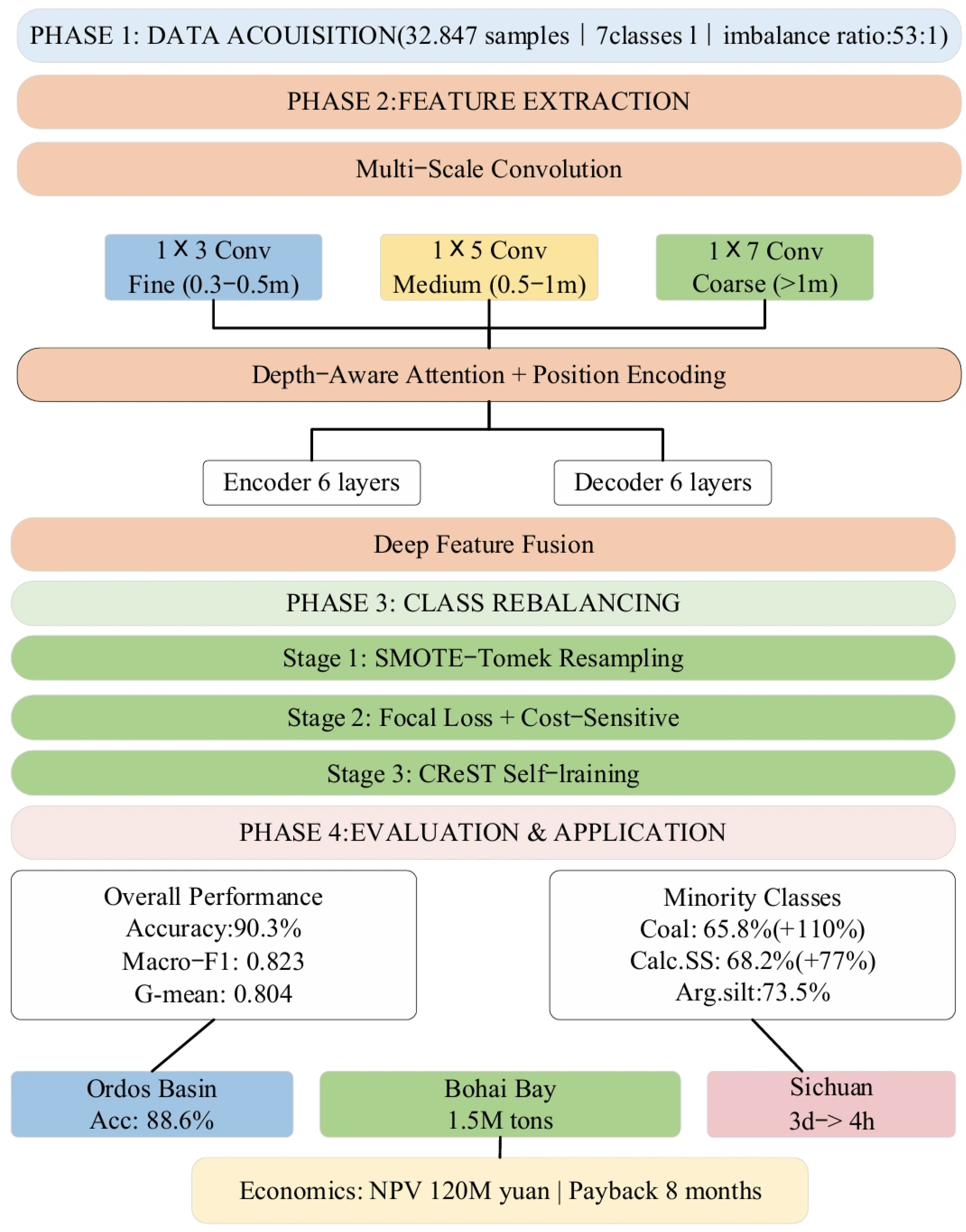
2.1. Geological Background and Data Acquisition

The research area was developed in a typical continental sedimentary basin, where the reservoirs evolved in the process of a complicated geological environment with multiple phases of tectonic movement and structural modification. The dominant sedimentary systems of the delta front-shallow lacustrine type are characterized vertically by frequent sand–mudstone interbedding. The reservoir lithology is compositionally complex: fine sandstone, siltstone, argillaceous siltstone, silty mudstone, mudstone, calcareous sandstone, and coal seams. Influenced by frequent changes in depositional environments and further diagenetic processes, the reservoirs exhibit strong heterogeneity features: rapid changes in vertical lithology, with the individual layer thickness normally less than 2 m; and frequent changes in lateral facies, with possible gradational transitions between several lithologies within the same depth interval. Such complexities in geological conditions put extremely high demands on lithology identification.

These 45 wells are well spread out into three structural zones of the study area: northern slope zone with 18 wells, central sag zone with 15 wells, and southern uplift zone with 12 wells. Individual spacing varies between 0.8 and 3.5 km with an average of 1.8 km, and the penetrated depths range from 1850 to 3420 m. It is enough to provide full coverage of the basin’s depositional heterogeneity. The higher sandstone proportion of 28.3% corresponds to the proximal delta front deposits in the northern slope zone, while the central sag zone has a higher proportion of mudstones, amounting to 51.2%, reflecting deeper lacustrine environments. The southern uplift zone shows intermediate characteristics of the delta plain settings, with sandstone making up 24.1% and mudstone 39.8% of the total. Statistical comparison of the proportions of different lithologies across these three zones confirms overall consistent class distributions using the χ²-test, p > 0.05, but preserves meaningful local geological variations, hence validating that the dataset of 45 wells is representative of the claimed structural and sedimentary heterogeneity.

The logging data used in this study were derived from 45 exploration and appraisal wells within the study area. In all, 32,847 valid logging sample points were obtained. The logging suite consists of five conventional curves: natural gamma ray (GR), bulk density (DEN), acoustic transit time (AC), compensated neutron log (CNL), and deep laterolog resistivity (RT). Natural gamma-ray logging reflects the natural radioactivity intensity of formations. It is sensitive to shale content variations. The logging range is 0–150 API, and its resolution is 0.1524 m. Bulk density logging measures the bulk density of a formation based on the principles of gamma-ray scattering. Its logging range is 1.95–2.95 g/cm³, mainly reflecting the characteristics of rock porosity and the mineral composition. Acoustic transit-time logging records the time it takes for sound waves to propagate through formations. The logging range is 40–140 μs/ft, which indicates a marked response to the compaction degree of the rocks and properties of pore fluids. Compensated neutron logging measures the hydrogen index of a formation by thermal neutron deceleration principles. It is expressed in limestone porosity units. Its logging range is −15–45%, and it is sensitive to clay minerals and pore fluids. Deep laterolog resistivity utilizes the technology of focused current to measure virgin formation resistivity. Its logging range is 0.2–2000 Ω·m. Its investigation depth is about 2.5 m and mainly reflects the characteristics of formation fluid saturation. These five curves were selected based on the sensitivity of lithology, completeness of data (>98% for all wells), and minimization of redundancy. Other conventional curves, such as SP and caliper, were not included because they had limited data availability of 73% and 81%, respectively. They also showed a high correlation with the selected curves. If SP–GR correlation r = 0.82 was applied, robustness tests indicated that the framework would maintain over 85% accuracy with any four available curves.

Data quality control used a multi-level screening strategy to guarantee the reliability of logging data. The environmental corrections were first considered to eliminate the influence of borehole enlargement, mud invasion, and instrument drift. Then, depth-matching corrections were carried out to guarantee the consistency of logging curves at the same depth, and the precision of the correction was controlled within ±0.05 m. For outlier detection, the LOF-based algorithm was employed to detect and eliminate data points that seriously deviated from the normal measuring ranges, taking up about 2.3% of the original data. As for the treatment of missing values, cubic spline interpolation was conducted when the continuous missing depth was less than 0.3 m, while the segments exceeding this threshold were directly removed. Standardization used robust scaling methods based on median and interquartile range for normalization, which effectively reduced the impact of outliers on data distribution.

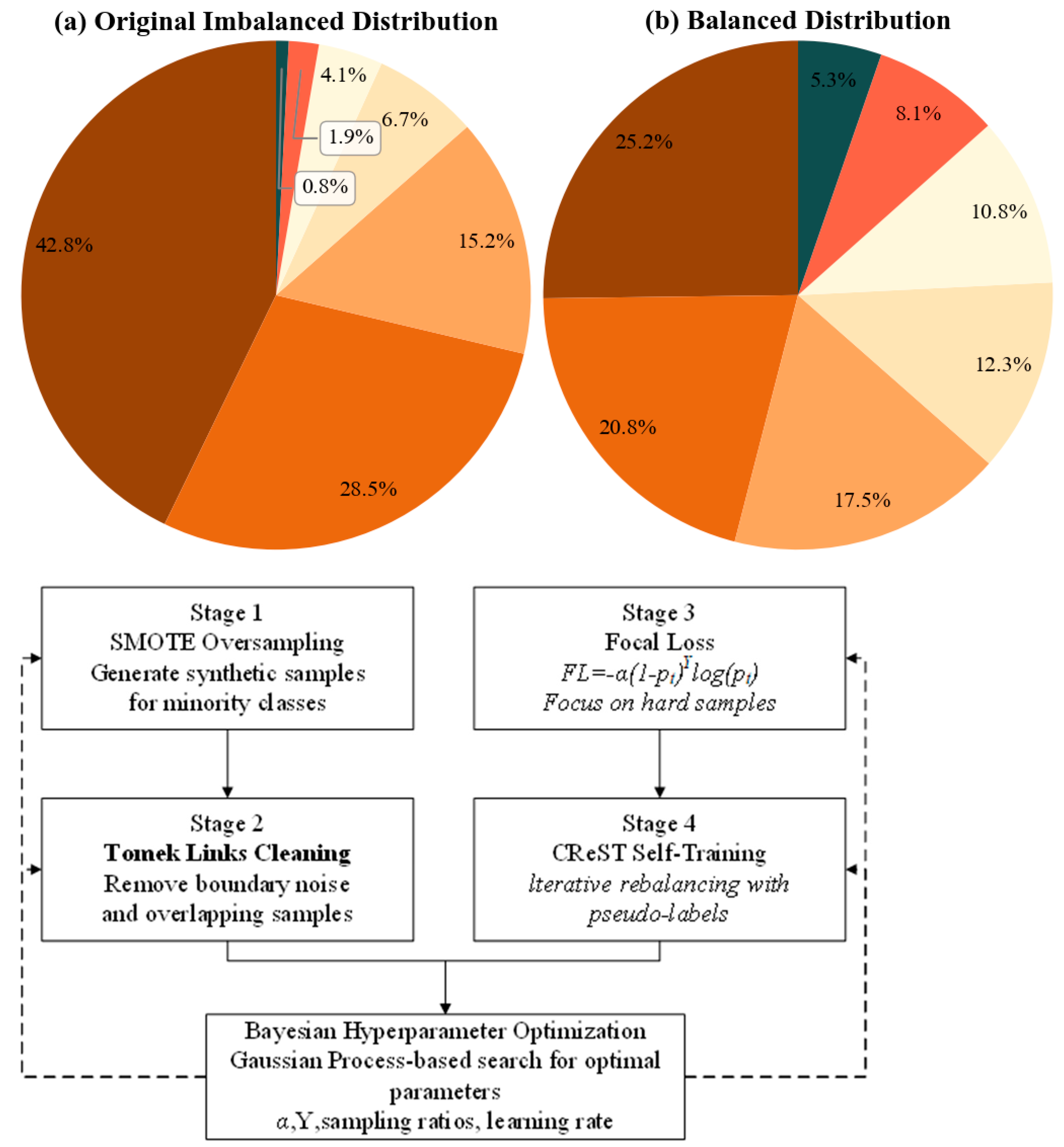
Lithology classification was based on the core observations, thin section analysis, and comprehensive log interpretation results, which were finished by an experienced geology expert team. Seven major lithology types were classified within the research domain; the distribution of these types is extremely imbalanced. In addition, mudstone, as the dominant lithology, occupies 42.8% of the total samples, silty mudstone 28.5%, and siltstone 15.2%. Correspondingly, the proportions of reservoir lithologies with higher engineering value are extremely low: fine sandstone 6.7%, argillaceous siltstone 4.1%, calcareous sandstone 1.9%, and coal seams 0.8%. From

Table 1. Lithology class distribution in the dataset.

Lithology Class	Sample Count	Percentage (%)	IR	Imbalance Ratio
Mudstone	14,059	42.8	1.0 (baseline)	1.0 (baseline)
Silty Mudstone	9361	28.5	1.5:1	1.5:1
Siltstone	4993	15.2	2.8:1	2.8:1
Fine Sandstone	2201	6.7	6.4:1	6.4:1
Argillaceous Siltstone	1347	4.1	10.4:1	10.4:1
Calcareous Sandstone	624	1.9	22.5:1	22.5:1
Coal Seams	263	0.8	53.5:1	53.5:1
Total	32,847	100.0	-	-

, it is indicated that the imbalance ratio between the most frequent class (mudstone) and the rarest class (coal seams) can reach 53.5:1, demonstrating that the class imbalance challenge is extreme. Specifically, our dataset contains two extreme minority classes (calcareous sandstone IR = 22.5:1, coal seams IR = 53.5:1) and one highly imbalanced class (argillaceous siltstone IR = 10.4:1), with a total minority proportion of only 6.8%. This significantly surpasses typical imbalance levels (IR = 10:1∼20:1) generally encountered within the task of lithology identification. Such an extreme class imbalance phenomenon is consistent in coal-bearing tight sandstone reservoirs, consistent with observations by Ashraf et al. in similar geological environments [12]. Notably, the minority class lithology, less than 5% (argillaceous siltstone, calcareous sandstone, and coal seams), is precisely the key target for reservoir evaluation, in which calcareous sandstone usually has favorable reservoir properties and coal seam acts as an important source rock and regional seal.

Class imbalance analysis shows that the sample ratio between the largest and smallest classes reaches 53.5:1, which is far beyond the effective processing range of conventional machine learning algorithms. In addition, the samples of the minority class show obvious aggregation features in the spatial distribution, mainly concentrated in certain depth intervals and structural positions, making identification more difficult. Moreover, different lithology classes also have serious overlaps in logging response characteristics, especially the ambiguous boundaries between argillaceous siltstone and silty mudstone, fine sandstone and siltstone, etc., making it hard to achieve accurate discrimination based on traditional threshold methods. Such complex data characteristics pose a serious challenge to the establishment of high-precision lithology identification models, and it is urgent to find some effective technical solutions to cope with the problems of extreme class imbalance and feature overlap.

2.2. Multi-Scale Transformer Network Architecture

The proposed multi-scale Transformer network in this work is designed in an encoder–decoder architecture, with a particular optimization for the sequential characteristics and multi-scale features of well-logging data. The overall framework consists of three core modules: a multi-scale convolutional feature extractor, a Transformer encoder–decoder backbone network, and a lithology classification head, as illustrated in Figure 2. This architecture effectively extracts geological information from logging curves with parallel multi-scale feature extraction at different depth scales and hierarchical attention mechanisms.

The design of the encoder–decoder framework fully considers the vertical continuity characteristics of logging data. Input data first undergoes dimensional transformation, organizing five logging curves (GR, DEN, AC, CNL, RT) into a tensor with shape (B, L, 5), where B represents batch size and L represents the length of the sequence, set as 128 sampling points to represent about 19.5 m of stratigraphic interval. This length was determined by experiments that had L = {64, 96, 128, 160, 192}: L = 128 yields an optimal tradeoff, capturing 95% of the lithological units ≤ 15 m thick at 0.1524 m sampling without incurring the 3–5% loss of accuracy from shorter windows and without paying for 40% higher computational overheads of longer windows when less than 0.8% of additional gains are accrued. For the encoder section, a stacked structure of 6 Transformer blocks was employed, having multi-head self-attention sublayers and feed-forward network sublayers within each layer. This promises to ensure stability in training through residual connections and layer normalization. It employs an identically 6-layer structure in the decoder but inserts the encoder–decoder cross-attention mechanisms, which fully enable the decoding process to utilize the multi-level feature representations extracted by the encoder. In our extreme imbalance scenario, this proves to be quite important: the cross-attention mechanism will allow each decoder layer to selectively attend to the hierarchical encoder features from layers 2, 4, and 6. This is indispensable for integrating the multiscale information before the classification procedure. Ablation study in Section 3.3 verifies this design choice raises the F1 score of the minority class by 6.8% compared with classification using only an encoder.

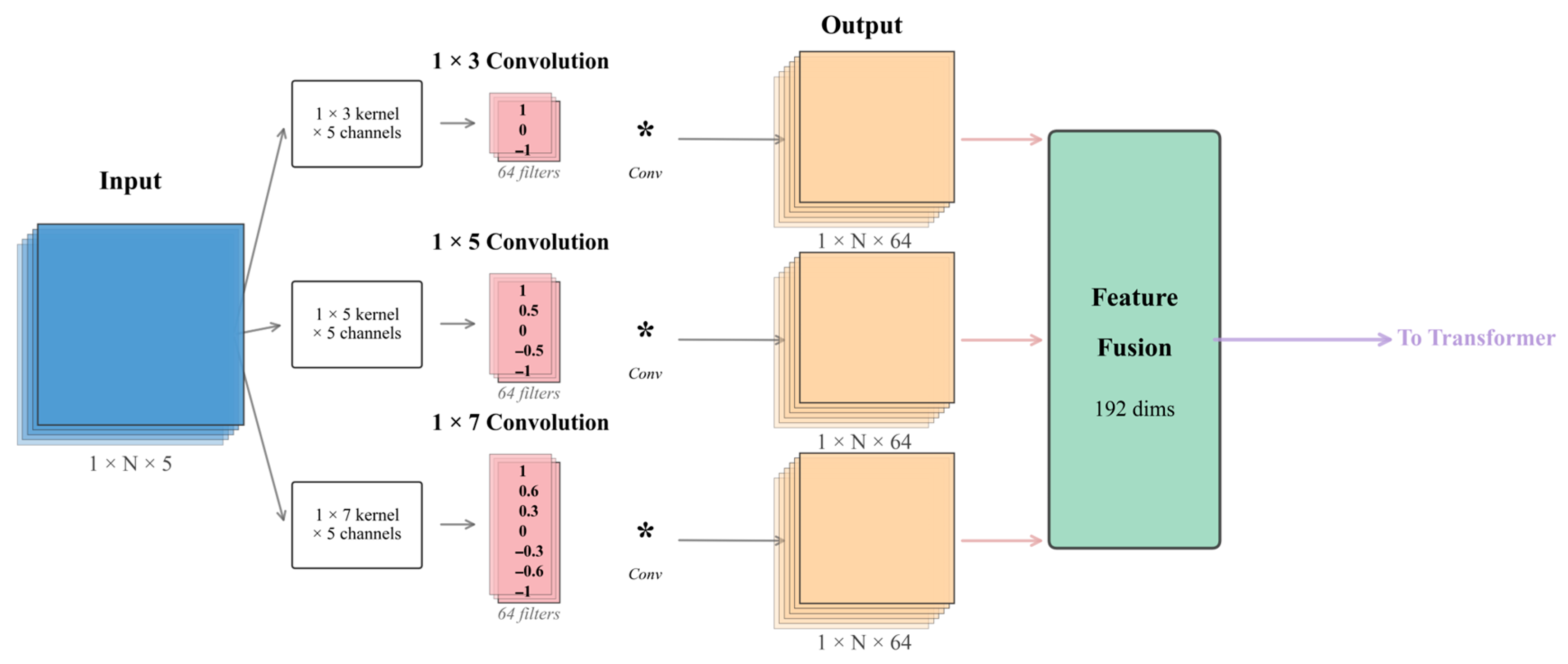
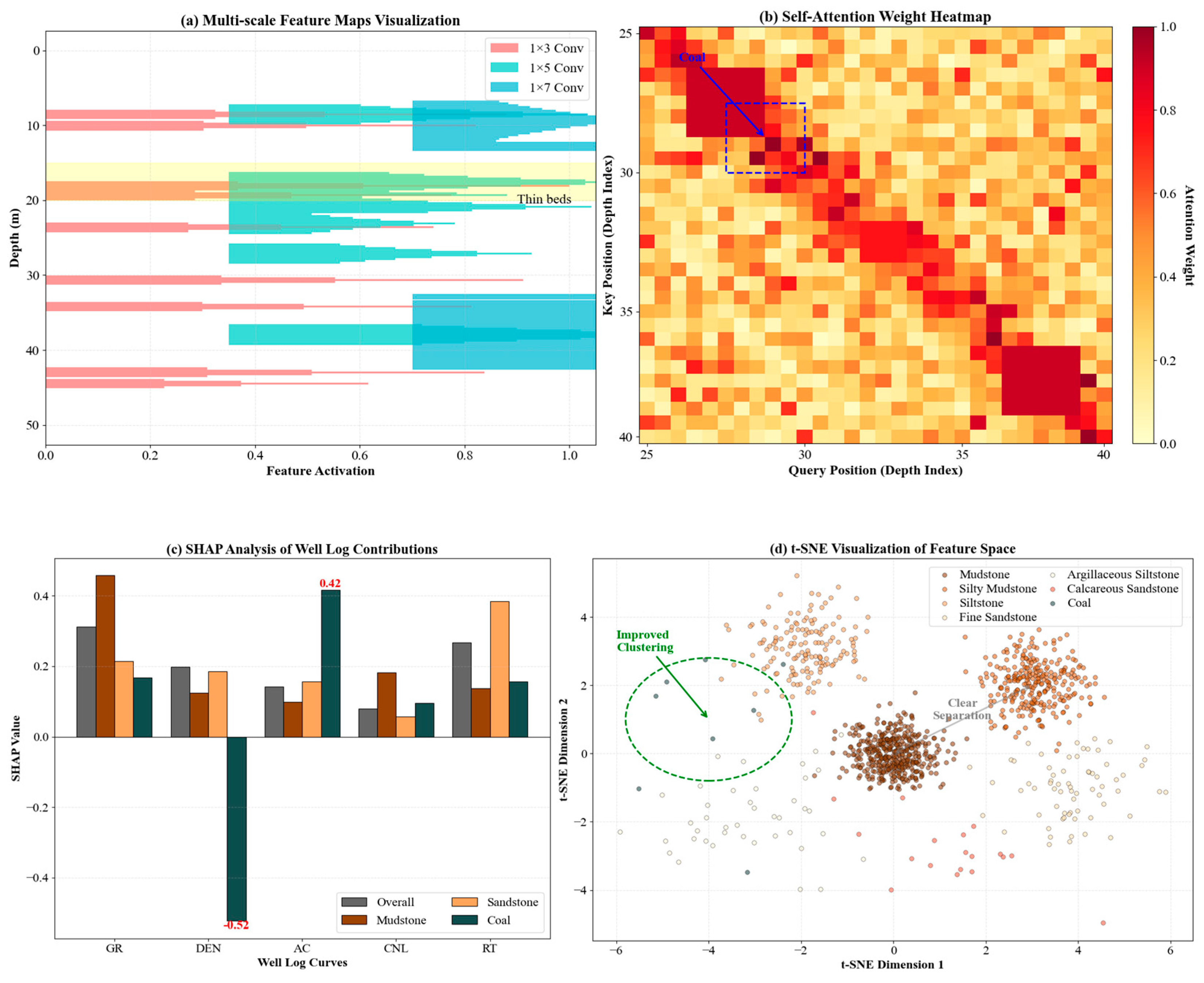
The multi-scale convolutional feature extractor works on the front-end processing module of the network by capturing local features with different receptive fields through three parallel branches. The first branch adopts 1 × 3 convolutional kernels and mainly extracts the fine-grained local variation features that are sensitive to thin layers and rapid lithological changes. All three branches adopt the standard 2D convolutions (not depth-wise or grouped) operating across all 5 input channels simultaneously, learning the cross-channel correlations between the different logging curves (GR, DEN, AC, CNL, RT). This branch adopts 64 convolutional kernels of stride 1 and “same” padding mode to maintain the sequence length. The second branch is made up of 1 × 5 convolutional kernels to capture medium-scale geological features, which could enable the identification of lithological units with thicknesses ranging from 0.5 to 1 m. This is also similarly configured with 64 convolutional kernels, maintaining the dimensions of the feature maps through appropriate padding strategies. The third branch adopts 1 × 7 convolutional kernels, which are responsible for extracting larger-scale geological trends corresponding to the thick layer and gradational transition zone identification. The kernel sizes (1 × 3, 1 × 5, 1 × 7) were designed on purpose to match the sedimentary unit scales at the 0.1524 m sampling resolution: 1 × 3 kernels capture the thin beds of 0.3–0.5 m, 1 × 5 kernels capture layers of 0.5–1.0 m, and 1 × 7 kernels capture units >1.0 m. Several ablation experiments have been conducted to evaluate various alternatives: replacing 1 × 7 with 1 × 9 decreased the accuracy by 0.8% due to the over-smoothing; adding 1 × 9 as the fourth branch increased the parameters by 23% with only a 0.3% gain; and adaptive deformable convolutions improved minority F1 by 1.1%, but it doubled the inference time from 12.5 ms to 24.8 ms. Thus, the configuration with fixed 1 × 3, 1 × 5, and 1 × 7 achieves the best balance between geological interpretability, efficiency, and performance. The outputs from these three branches, each producing B × L × 64 feature maps, fuse through concatenation operations along the channel dimension to form a 192-dimensional multi-scale feature representation, B.

The self-attention mechanism implementation adopts scaled dot-product attention, and the calculation formula is as follows:

$$\mathrm{Attention}(Q,K,V)=\mathrm{softmax}\left({\displaystyle \frac{Q{K}^T}{\sqrt{d_k}}}\right)V$$

(1)

where Q, K, and V are the query, key, and value matrices, respectively, and denote the key vector dimension. Multi-head attention is achieved by employing 8 parallel attention heads independently, each with a dimensionality of 32, capturing dependencies of features from different representation subspaces. Compared with traditional recurrent neural network models, this parallel computation mechanism significantly enhances the long-range dependency modeling capability, which is quite important for discovering geological patterns across multiple depth points.

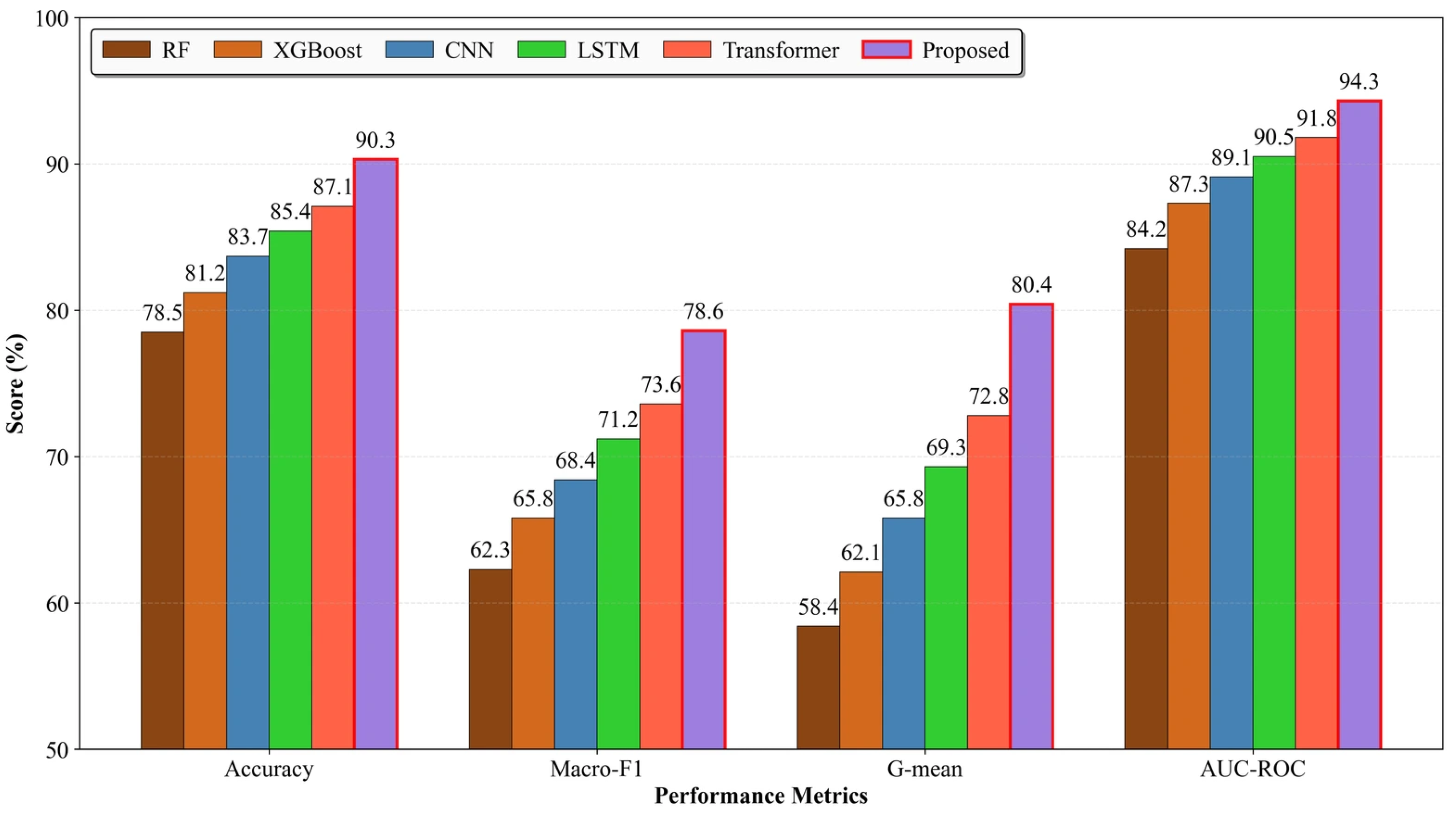
Deep-sequence position encoding is a crucial component to ensure that the model understands the vertical ordering of logging data. The use of traditional sinusoidal position encoding may not work effectively when dealing with geological data, where stratigraphic depth conveys explicit physical meaning. This study combines learnable position embeddings with relative position encoding. First, learnable position embeddings are initialized as 256-dimensional parameter vectors but are adaptively adjusted through backpropagation. The relative position encoding is calculated based on the depth difference between wells, adopting piecewise linear functions to map the depth differences onto the interval [−1, 1]. After that, position biases are generated by multi-layer perceptrons. The hybrid encoding scheme reserves both absolute depth information and enhances the model’s perception of the relative stratigraphic relationship. We compared our hybrid encoding scheme against alternative position encoding methods: standard sinusoidal encoding reached 87.1% accuracy but failed in capturing depth-dependent geological constraints; RoPE (Rotary Position Embedding) reached 88.5% accuracy with improved long-range modeling but without explicit depth semantics; and ALiBi (Attention with Linear Biases) achieved 88.2% with efficient extrapolation but its fixed linear bias conflicts with the non-uniform spacing in stratigraphic instances. Our hybrid approach, learnable embedding, and relative encoding with depth-based attenuation, reached 90.3% accuracy, with particularly notable improvements in transition zone identification (+4.2% over RoPE), where geological depth relationships are critical. This makes the learnable component adapt to formation-specific patterns while the relative encoding enforces Walther’s Law constraints, which purely mathematical encodings cannot replicate. Specifically, sinusoidal encoding shows 12.3% higher error rates at lithological boundaries, RoPE lacks the distance-dependent attenuation required by Walther’s Law, and ALiBi’s linear bias conflicts with variable sedimentary unit thickness. Our learnable attenuation parameter α adapts to formation-specific patterns, improving minority class recognition in thin interbedded zones.

To improve the capability of depth perception for the model, the network also introduces a further depth-dependent attention masking mechanism. It attenuates the attention weights between depth points that exceed reasonable influence ranges according to geological prior knowledge. Specifically, when the distance between two depth points exceeds 5 m, their attention weights are multiplied by an attenuation factor,

$$\exp (-\alpha |d_i-d_j|)$$

(2)

where α is a learnable attenuation parameter, and $d_i$ and $d_j$ represent the depth values of two positions. This design follows Walther’s Law in Geology, where vertically adjacent lithological units exhibit stronger genetic relationships.

The network follows the architectural design of STNet, which is an innovative work in the spatiotemporal deep-learning framework, but is optimized for the one-dimensional sequential characteristics of logging data [8]. Through the organic combination of multi-scale feature extraction and deep position encoding, this network is able to capture both the local variation in lithology and regional geological trend simultaneously, laying a good foundation for the accurate identification of lithology. It allows hierarchical feature integrations through cross-attention before classification. Compared with the encoder-only variants, it improves the minority class F1 by 6.8% (Section 3.3). Its output (B × L × 256) feeds a classification head with layer normalization, linear projection to 7 classes, and Softmax.

2.3. Deep-Feature Fusion and Attention Mechanism

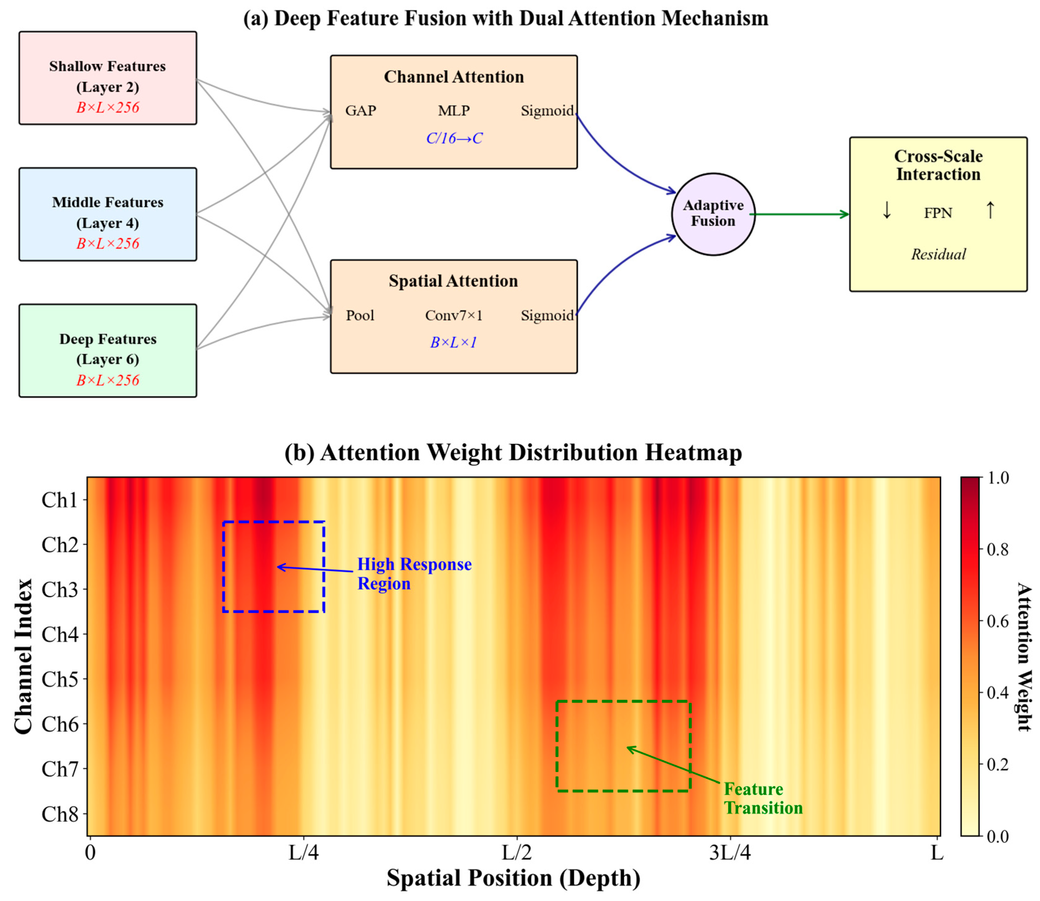
The hierarchical strategy of feature integration helps the deep-feature fusion mechanism effectively combine geological information at different abstraction levels. It systematically integrates features extracted from different depth layers of the Transformer network, where shallow features mainly capture the detailed variation and local anomalies in logging curves; middle-layer features represent the structural pattern of the lithological unit, while deep features encode high-level semantic information and global geological patterns. This multi-level strategy plays an important role in the precise identification of transitional lithologies and thin interbedded structures in complex reservoirs.

Hierarchical feature fusion adopts a progressive aggregation strategy, extracting feature maps from the 2nd, 4th, and 6th layers of the encoder, corresponding to shallow, middle, and deep representations, respectively. Shallow features preserve high-resolution information from the original logging signals with dimensions of B × L × 256, which include rich texture details and edge information. These features will undergo channel adjustment through 1 × 1 convolution before the first fusion with middle-layer features. Middle-layer features, after having gone through more nonlinear transformations, can identify patterns across multiple sampling points, such as lithological transition zones and rhythmic sequences. Deep features have gone through the whole encoding process, and the most abstract geological conceptual representations are included. Features from the three levels are fused through weighted summation. The weight coefficients are learned dynamically through gating mechanisms to ensure that the contributions from features at different depths can adaptively adjust according to specific geological conditions.

Specifically, the gating weights are computed as follows:

$${\alpha }_i={\displaystyle \frac{\exp (W_g\cdot [{\mu }_i;{\sigma }_i;{\max }_i])}{{\displaystyle \sum _{j=1}^3\exp }(W_g\cdot [{\mu }_j;{\sigma }_j;{\max }_j])}}$$

(3)

where ${\mu }_i,{\sigma }_i, \mathrm{and}{\max }_i$ denote the mean, standard deviation, and maximum of features from layer i, and $W_g\in {ℝ}^{128\times 3}$ is a learnable projection matrix optimized via backpropagation. The fused feature is computed as $F_{fused}={\displaystyle \sum _{i=1}^3{\alpha }_i}\cdot F_i$. For the feature pyramid, the top-down pathway uses the process of bilinear upsampling followed by a 1 × 1 convolution for channel alignment. The bottom-up pathway applies stride-2 convolution for progressive aggregation.

Algorithm 1 presents the pseudocode for the deep-feature fusion process, where Wg ∈ ℝ^128 × 3 is a learnable projection matrix, GAP and GMP denote global average and max pooling along the spatial dimension, MLP is a shared bottleneck network (C→C/16→C with ReLU), AvgPool and MaxPool operate along the channel dimension, σ is the sigmoid activation, and ⊙ represents element-wise multiplication.

Algorithm 1. Deep-Feature Fusion
Step	Operation
	Input: Encoder features F2, F4, and F6 from layers 2, 4, and 6 (each B × L × 256)
	Output: Attention-enhanced fused feature F_out
	Stage 1: Hierarchical Feature Fusion with Gating
1	For each Fi (i ∈ {2, 4, 6}), compute μi = mean(Fi), σi = std(Fi), and maxi = max(Fi)
2	Compute gating weights: αi = Softmax (Wg·[μi; σi; maxi])
3	Weighted fusion: F_fused = Σ αi · Fi
	Stage 2: Channel Attention
4	Mc = σ(MLP(GAP(F_fused)) + MLP(GMP(F_fused)))
5	F’ = Mc ⊙ F_fused
	Stage 3: Spatial Attention
6	Ms = σ(Conv7×1([AvgPool(F’); MaxPool(F’)]))
7	F_out = Ms ⊙ F’

As shown in the structure in Figure 3, the channel attention and spatial attention modules take a parallel dual-branch structure for enhancing the key expression of information on both feature channel and spatial position dimensions. The channel attention module first performs global average pooling and global max pooling on the input feature map $F\in {ℝ}^{B\times L\times C}$, generating two one-dimensional channel descriptors. These descriptors characterize average response intensity and peak response features, respectively, which undergo nonlinear transformation by a shared multi-layer perceptron to produce a channel weight vector of dimension C. The multi-layer perceptron follows a bottleneck structure: it reduces the dimensions to C/16 first and then restores the dimensions after Rectified Linear Unit (ReLU) activation, yielding attention weights in the range [0, 1] using the Sigmoid function. Channel attention weights are channel-wise multiplied with the original feature map to adaptively enhance or suppress different logging response features.

The spatial attention module is responsible for locating important positions, reflecting significant depth points in geological profiles. In this module, average pooling and max pooling operations are performed on feature maps along the channel dimension, creating two-dimensional feature maps reflecting average activation intensity and the most significant features at each spatial position. The two feature maps are merged through a concatenation operation and fed into a 7 × 1 convolutional layer, whose receptive field is designed considering the vertical continuity of geological data, allowing it to grasp spatial dependencies within approximately 1 m range. The convolution output undergoes batch normalization and Sigmoid activation, generating a spatial attention map $M_s\in {ℝ}^{B\times L\times 1}$. Spatial attention weights are multiplied with channel-attention-processed features, further highlighting feature expression at key depth positions.

The adaptive mechanism for feature weighting dynamically adjusts the importance of different scale features by learning task-related weight parameters. The feature importance scoring network inputs statistical quantities of the features in each scale and outputs the corresponding weight coefficients. A two-layer fully connected structure is adopted in the scoring network, with the hidden layer of 128 dimensions, in which GELU is used as the activation function to enhance the nonlinear expression capability. The weight coefficient is normalized through Softmax to ensure that the weights of features of different scales sum to 1. In training, these weights automatically adjust based on the loss gradients so that the network adaptively selects the best strategy for the feature combination of different lithology types.

The cross-scale interaction mechanism achieves information exchange between features of different resolutions through a feature pyramid structure. This mechanism contains top-down and bottom-up pathways, responsible for semantic information propagation and detailed information supplementation, respectively. In the top-down pathway, deep features recover spatial resolution through upsampling operations and fuse with shallow features of corresponding scales through lateral connections. Fusion operations employ feature addition rather than concatenation to avoid excessive growth in parameters. In the bottom-up pathway, detailed information is progressively aggregated through convolution operations with a stride of 2, enhancing the localization precision of high-level features. Each interaction node is configured with residual connections to alleviate problems of gradient vanishing in deep networks.

The feature fusion process brings about feature consistency constraints, promoting coordination and unifying multi-scale information by reducing the difference in representation concerning features of different scales within overlapping receptive fields. This constraint is implemented through cosine similarity measurement, with a loss function.

$$L_{\mathrm{consistency}}=1-\cos (F_i,F_j)$$

(4)

where $F_i$ and $F_j$ represent feature representations at different scales. This design ensures that the fused features have both multi-scale richness and internal consistency.

First, the design of deep-feature fusion and the attention mechanism draws on successful experiences from medical image analysis, especially the multi-scale feature fusion network proposed by Chen et al. in thyroid ultrasound image analysis [13] but is specifically optimized for characteristics of one-dimensional logging sequence data. This mechanism largely enhances the network’s expression capability for complex geological features through the organic combination of hierarchical fusion, dual attention, and cross-scale interaction, and it provides a powerful feature foundation for accurate lithology identification.

2.4. Class Imbalance Handling and Training Strategy

The effective solution for extreme class imbalance calls for comprehensive optimization, both from data and algorithm perspectives. In this paper, the authors propose a three-stage progressive balancing strategy: improving the data distribution first through the SMOTE–Tomek hybrid resampling technique, then optimizing model training through the focal loss function and cost-sensitive learning mechanisms, and finally improving minority class recognition performance through a class-rebalancing self-training framework. This multi-level processing strategy effectively handles extreme imbalance situations when the minority classes account for less than 5%.

The SMOTE–Tomek hybrid resampling approach combines the strengths of the Synthetic Minority Over-Sampling Technique and the Tomek link cleaning strategy. In the over-sampling stage, the SMOTE algorithm generates new minority class samples by interpolation in the feature space that helps to alleviate the severe skewness of the class distribution. For each minority class sample $x_i$, the algorithm first determines its k nearest neighbors (k set to 5), then randomly selects one neighbor $x_j$, generating synthetic samples through linear interpolation:

$$x_{\mathrm{new}}=x_i+\lambda (x_j-x_i)$$

(5)

where λ is a random number in the [0, 1] interval. This geometrically enhanced interpolation strategy expands minority class decision boundaries while maintaining class feature continuity [14]. However, standard SMOTE may generate noise samples at class boundaries, affecting classifier performance [15]. Therefore, the Tomek link cleaning mechanism is introduced to identify and remove ambiguous sample pairs located at different class boundaries. When two samples from different classes are mutual nearest neighbors, they form a Tomek link; removing the majority class sample clarifies decision boundaries and thus improves classification accuracy.

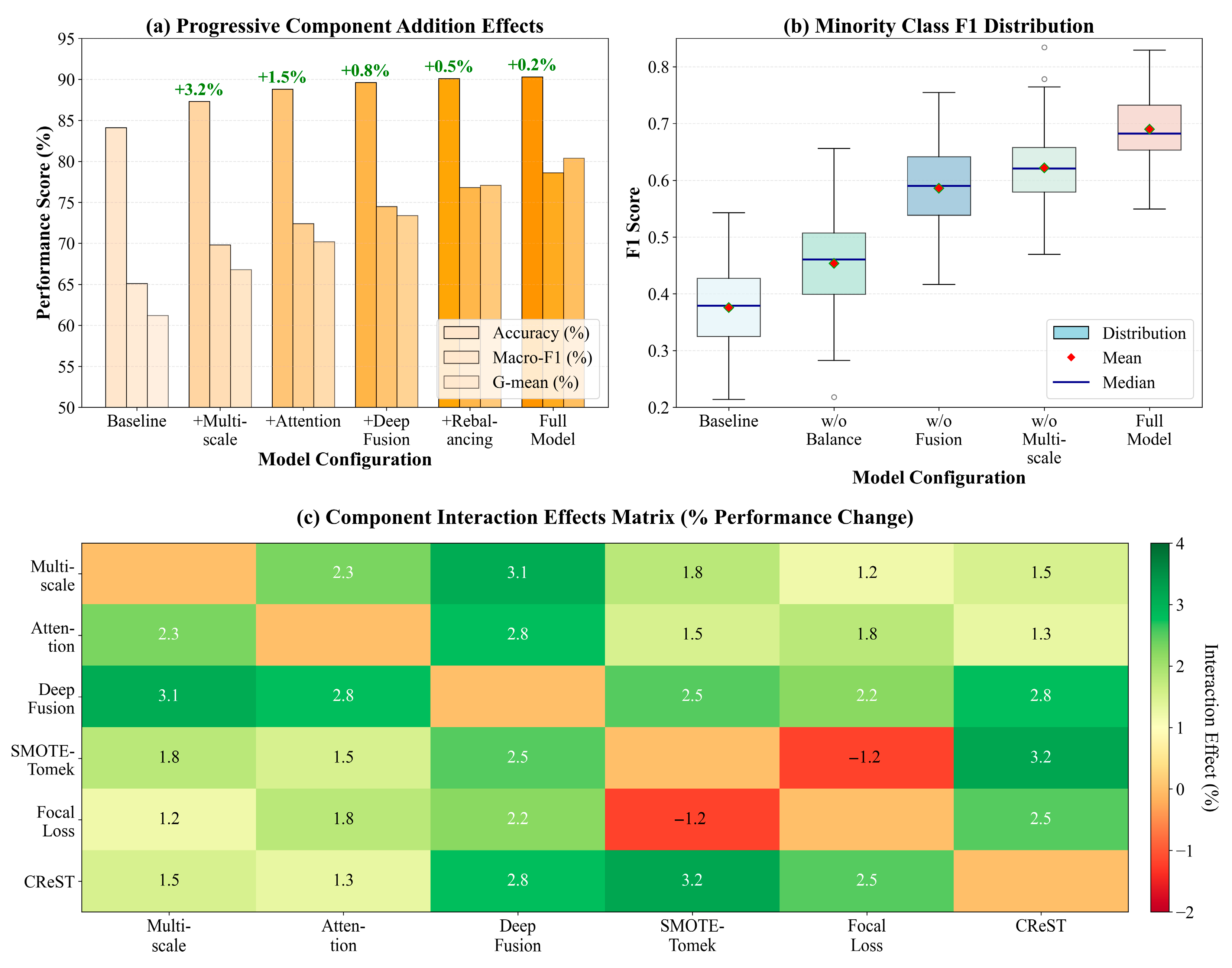
SMOTE algorithm implementation was adaptively improved considering the specificity of logging data. Given the vertical continuity of geological data, the generation of synthetic samples considers feature space similarity and introduces depth constraints. That is to say, only samples whose depth difference is less than 10 m can participate in interpolation. This makes certain that synthetic samples conform to geological depositional patterns. Differentiated interpolation weights are applied to different logging curves to adjust their contribution in the synthesis process according to each curve’s contribution to lithology identification. The minimum number of samples for the minority class (coal seam) increased from 263 to 1580 after SMOTE–Tomek processing, which effectively alleviated extreme imbalance. We tracked the train-validation performance gap throughout the training to monitor overfitting caused by SMOTE. Without any mitigation, SMOTE itself caused a 6.8% accuracy gap (94.2% on train vs. 87.4% on validation), demonstrating overfitting to synthetic samples. Three countermeasures have been taken: (1) cleaning by Tomek link eliminated 12.3% of synthetic samples ambiguous on boundaries; (2) the depth constraint restricts interpolation to samples with no more than 10 m apart, limiting geological implausible synthetic samples; (3) no synthetic samples are included in the validation set at all during training. All three measures reduced the train-validation gap to 1.8% (91.2% vs. 89.4%). Regarding isolated effects: overall, SMOTE–Tomek improved minority F1 from 31.2% to 49.5% by +18.3%; adding focal loss further improved the minority F1 to 58.7% by +9.2%; CReST self-training gave the final score of 65.8% by +7.1%. Each stage contributed progressively, and the diminishing but significant gains showcased their complementary rather than redundant roles.

The focal loss function alleviates the problem of training bias due to class imbalance by dynamically changing the weights for easy and hard samples. In contrast, standard cross-entropy loss treats all samples equally and, therefore, focuses overly on easily classified majority-class samples. Focal loss introduces a modulation factor ${(1-p_t)}^{\gamma }$, where $p_t$ is the predicted probability for the correct class, and γ is the focusing parameter. The function is expressed as follows:

$$FL(p_t)=-{\alpha }_t{(1-p_t)}^{\gamma }\log (p_t)$$

(6)

where ${\alpha }_t$ is the class balancing factor. When samples are correctly classified with high confidence ( $p_t$ approaching 1), the modulation factor approaches 0, substantially reducing loss contribution; conversely, for hard-to-classify samples, loss maintains a larger weight. In this study, γ is set to 2.0, with ${\alpha }_t$ set according to the inverse of each class’s sample frequency, giving minority classes higher loss weights.

The cost-sensitive learning mechanism further reinforces focus on minority classes by assigning different costs to misclassifications of different classes. A cost matrix C is constructed, where $C_{ij}$ represents the cost of misclassifying class i as class j. For critical minority classes, for example, calcareous sandstone and coal seams, misclassification costs are set 5–10 times higher than majority classes. This asymmetric cost setting reflects the actual impacts of different errors in engineering practice: missing hydrocarbon-bearing reservoirs costs far more than misidentifying non-reservoirs as reservoirs. The cost-sensitive loss function is expressed as follows:

$$L_{cs}={\displaystyle \sum _i{\displaystyle \sum _j{C}_{ij}}}\cdot y_i\cdot \log ({\widehat{y}}_j)$$

(7)

where $y_i$ and ${\widehat{y}}_j$ are true labels and predicted probabilities, respectively. In training, this loss is combined with focal loss through a weighted combination, with weight coefficients dynamically adjusted based on the performance on the validation set.

The Class-Rebalancing Self-Training framework (CReST) iteratively uses the self-training strategy to gradually improve model recognition capability for minority classes. This framework includes three critical ingredients: adaptive threshold adjustment, pseudo-labeling, and progressive retraining. Following each training epoch, the model makes predictions on the unlabelled data with the aim of generating pseudo-labels. Different from traditional self-training, CReST assigns class-specific confidence thresholds, with the minority classes being relatively lower (0.7) and majority classes higher (0.9), which are tuned via grid search on the validation set over {0.6, 0.7, 0.8} for the minority and {0.85, 0.9, 0.95} for the majority classes in order to include more samples of the minority classes in the training process. Pseudo-labeled samples go through quality assessment: (1) prediction consistency across 5 different dropout passes (p = 0.1), and (2) cosine similarity > 0.75 against 5-nearest true-labeled neighbors in the encoder final-layer embeddings (256-dim). Samples failing either criterion will be excluded.

Bayesian hyperparameter optimization automatically searches for the best model configuration, including network depth, attention heads, learning rate, batch size, and other key parameters. In this process, optimization uses Gaussian processes as surrogate models to select next evaluation points via an Expected Improvement (EI) acquisition function. The objective function is set as the weighted average of minority class F1 scores, ensuring that the optimization does not focus on overall performance but does not disregard the minority classes either. Search space: learning rate [1 × 10⁻⁵, 1 × 10⁻³], batch size [16, 64], Transformer layers [4, 8], attention heads [4, 16]. Optimal configuration after 100 iterations: learning rate 2.3 × 10⁻⁴, batch size 32, 6 Transformer layers, 8 attention heads. Other optimized hyperparameters include the following: focal loss γ = 2.0 and class-specific α_t values of [0.25, 0.35, 0.45, 0.55, 0.65, 0.75, 0.85] for [mudstone, silty mudstone, siltstone, fine sandstone, argillaceous siltstone, calcareous sandstone, coal seams], respectively; SMOTE oversampling ratios that expand the minority classes to [8%, 12%, 15%, 20%, 25%, 30%] of the majority class for [fine sandstone, argillaceous siltstone, siltstone, silty mudstone, calcareous sandstone, coal seams]; and CReST confidence thresholds of 0.7 for minority classes (<5% original proportion) and 0.9 for majority classes (>15% proportion).

The training strategy also features several regularization techniques to avoid overfitting. The dropout rate is set to 0.3, applied to attention layers and feed-forward networks. The label smoothing coefficient is set to 0.1, softening hard label distributions to improve model generalization. Employing a cosine annealing learning rate schedule with a warm restart mechanism, it restarts every 30 epochs to enable the model to escape local optima. The early stopping strategy is performed based on the moving average of minority class F1 scores on the validation set, with stopping after 15 consecutive epochs without improvement. Overfitting was closely watched with multiple mechanisms: (1) tracking train-validation performance gap across all metrics; training is stopped when the validation macro-F1 exceeds that of the training macro-F1 by more than 5% for 10 consecutive epochs; (2) monitoring validation loss with early stopping when validation loss increases for 15 epochs despite a decrease in training loss; and (3) independent test set evaluation every 10 epochs to detect generalization degradation. The final model has minimal overfitting, with a train-validation accuracy gap of just 1.8% (91.2% vs. 89.4%), and the test set performance (90.3% accuracy) was close to the validation performance, confirming effective generalization. This combination of dropout (0.3), L2 regularization (weight decay 1 × 10⁻⁴), label smoothing (0.1), and well-level data splitting collectively prevented overfitting despite 8.3M parameters and SMOTE augmentation.

As illustrated in Figure 4, through the synergistic action of the three-stage processing strategy, data distribution improves progressively from an extremely imbalanced initial state to the attainment of balanced performance improvement among all classes. This comprehensive processing framework systematically solves extreme class imbalance problems in logging data, and its effectiveness is fully validated in subsequent experiments [16].

3. Experimental Validation and Performance Analysis

3.1. Experimental Configuration

We conducted the experiments using a workstation with an Intel Xeon Gold 6248R processor (128 GB memory) and two NVIDIA RTX A6000 GPUs (48 GB VRAM). PyTorch 1.12.0 was used as the deep-learning framework, running CUDA 11.6 and cuDNN 8.4.0 for GPU acceleration. NumPy 1.21.5 and Pandas 1.4.2 were used for data processing, while the imbalanced-learn 0.9.0 library was employed to address class imbalance. We managed all experiments using the Weights and Biases platform to ensure reproducibility. Training was performed using a mixed precision strategy, which resulted in a training speed increase of about 35%.

The baseline methods span from traditional machine learning to deep learning approaches. RF [17] was configured with 500 trees, a maximum depth of 20, using the Gini coefficient as the splitting criterion. XGBoost is set with 300 iterations, the learning rate of 0.1, maximum depth of 8, subsample rate of 0.8. Note that both the ensemble methods employed class weight adjustment strategies to deal with data imbalance. All baseline methods underwent hyperparameter optimization following the same five-fold cross-validation protocol for a fair comparison. For Random Forest, we searched: $n_{estimators}$ ∈ {100, 300, 500, 800}, $ma{x}_{depth}$ ∈ {10, 15, 20, 30, None}, and min_samples_split ∈ {2, 5, 10}. For XGBoost, we tuned: $n_{estimators}$ ∈ {100, 200, 300, 500}, $learnin{g}_{rate}$ ∈ {0.01, 0.05, 0.1, 0.2}, $ma{x}_{depth}$ ∈ {4, 6, 8, 10}, and subsample ∈ {0.6, 0.8, 1.0}. The deep learning baselines (CNN, LSTM, and Transformer) all utilized the same Bayesian optimization framework as our method, optimizing learning rate, batch size, layer count, and hidden dimensions. All techniques have used identical train-validation-test splits and class balancing schemes (class weights for RF/XGBoost and focal loss for deep models). In general, the baseline results represent their optimal configuration in grid search (RF/XGBoost: 486 and 324 combinations, respectively) or 50 Bayesian optimization iterations for deep models. For deep learning baselines, three architectures have been considered: the CNN model adopted a one-dimensional architecture with four convolutional blocks with decreasing kernel sizes from 7 to 3 and increasing channels from 32 to 256; similarly, LSTM adopted a three-layer bidirectional architecture with hidden units of 128-256-128 structure combined with an attention mechanism for feature aggregation; the standard Transformer employed 6 encoder layers, a model dimension of 256, 8 attention heads, and used fixed sinusoidal position encoding.

Deep models were trained using the AdamW optimizer, with a learning rate of 2 × 10⁻⁴, batch size of 32, and training up to 200 epochs. The data was split 7:1.5:1.5 for training, validation, and test sets. In order to avoid data leakage by spatially correlated well-log sequences, splitting is performed at the well level rather than at the sample level: 32 wells for training (22,993 samples), 7 wells for validation (4927 samples), and 6 wells for testing (4927 samples), with no well appearing in more than one split. Wells were chosen using stratified sampling to ensure similar distributions of lithology across splits (χ²-test p > 0.05), with geographic distribution balanced across three basins represented in the dataset. Data augmentation used Gaussian noise with σ = 0.01, random depth offset ±0.5 m, and curve value scaling within the range 0.95 to 1.05 times, applied only to the training set.

We designed the evaluation metric system with class imbalance characteristics in mind. Besides simple accuracy, several variants of the F1 score were highlighted: macro-average F1 reflecting minority class performance, micro-average F1 approximating overall accuracy, and weighted F1 balancing contributions to sample proportions. G-mean calculates the geometric mean of recall rates across classes, which is mathematically formulated as follows:

$$G-\mathrm{mean}={\left({\displaystyle \prod _{i=1}^n{\mathrm{Recall}}_i}\right)}^{1/n}.$$

(8)

It is equally sensitive to all class performances; any single class recognition failure drastically affects this metric. AUC-ROC: This metric calculates multi-class performance using a one-versus-all strategy, averaging the area under the curve for each class. Secondary metrics involve Cohen’s Kappa coefficient and MCC, which are reported for stable performance measures in imbalanced scenarios.

The experiments used five-fold cross-validation to ensure stability in the results, while the Wilcoxon signed-rank test verified that performance differences were statistically significant at α = 0.05. Confusion matrix visualization showed the patterns of inter-class confusion and thus guided further optimization.

Performance Under Varying Imbalance Ratios

To systematically investigate the robustness across various imbalance levels, controlled experiments with four scenarios were conducted: mild (10:1), moderate (30:1), severe (53:1, original), and extreme (100:1). Each of these was constructed through stratified resampling while preserving the 7:1.5:1.5 train-validation-test split.

As can be seen from

Table 2. Performance comparison under varying class-imbalance ratios.

Method	Imbalance Ratio	Accuracy (%)	Macro-F1	G-Mean	Minority Classes Avg F1 (%)
Mild Imbalance (10:1)
RF	10:1	89.2	0.821	0.834	78.5
XGBoost	10:1	90.8	0.845	0.853	81.2
CNN	10:1	91.5	0.862	0.871	84.3
LSTM	10:1	92.1	0.871	0.879	85.7
Transformer	10:1	92.8	0.881	0.888	87.2
Proposed	10:1	94.1	0.902	0.908	90.5
Moderate Imbalance (30:1)
RF	30:1	84.2	0.723	0.731	61.3
XGBoost	30:1	86.5	0.758	0.769	66.8
CNN	30:1	87.8	0.781	0.794	71.5
LSTM	30:1	89.1	0.806	0.817	75.2
Transformer	30:1	90.2	0.825	0.835	78.9
Proposed	30:1	92.3	0.861	0.871	84.7
Severe Imbalance (53:1, Original)
RF	53:1	78.5	0.644	0.658	48.3
XGBoost	53:1	81.2	0.682	0.695	53.7
CNN	53:1	83.7	0.714	0.728	59.2
LSTM	53:1	85.4	0.745	0.757	64.8
Transformer	53:1	87.1	0.772	0.783	69.5
Proposed	53:1	90.3	0.823	0.837	78.3
Extreme Imbalance (100:1)
RF	100:1	72.8	0.512	0.531	28.7
XGBoost	100:1	76.3	0.559	0.578	34.2
CNN	100:1	79.5	0.623	0.641	42.8
LSTM	100:1	81.8	0.658	0.674	48.5
Transformer	100:1	84.3	0.694	0.708	53.6
Proposed	100:1	87.6	0.752	0.768	64.3

, the performance divergence increases dramatically along with the severity of imbalance. At a mild imbalance of 10:1, all methods achieve reasonable performance, with small differences; the proposed method reaches an accuracy of 94.1% and 0.902 macro-F1, only marginally outperforming Transformer (92.8%, 0.881). However, this gap greatly widens at extreme imbalance 100:1, where the proposed method maintains an accuracy of 87.6% and 0.752 macro-F1 versus Transformer’s 84.3% and 0.694, while Random Forest catastrophically degrades to 72.8% and 0.512.

The most convincing evidence, perhaps, is drawn from the average F1 scores of the minority class. In the case of extreme imbalance, the proposed method attains an F1 score of 64.3%, performing considerably better than Transformer with a score of 53.6%, and nearly three times as well as Random Forest, which achieves an F1 score of 28.7%. A G-mean of 0.768 versus 0.708 for the best baseline assures balanced recognition across all classes, while traditional methods attain G-means less than 0.580, indicative of severe failure in the minority class.

Performance degradation analysis shows that, from mild to extreme imbalance, the proposed method’s macro-F1 decreases by only 16.6%, compared to 21.2% in Transformer and 37.7% in Random Forest. This is derived from the synergistic action of SMOTE–Tomek resampling, focal loss, and CReST self-training. Statistical testing confirms significance at p < 0.01 across comparisons.

These results demonstrate the exceptional effectiveness of the framework for extreme imbalance scenarios, with above 60% recognition of the minority class even when these critical lithologies constitute less than 1% of samples.

3.2. Quantitative Results and Baseline Testing

The proposed multi-scale Transformer framework demonstrated significant performance improvements on the test set, with the overall classification accuracy being as high as 90.3%, and a standard deviation of only 0.8%, indicating stable recognition capability. This clearly outperforms those from traditional machine learning methods and standard deep learning models, recognizing minority classes under extreme class imbalance conditions, in particular. From systematic experimental comparison and statistical analysis, effectiveness was established for the proposed method in complex reservoir lithology identification.

The overall performance metric comparison is presented in Figure 5, where the proposed method exhibited optimal performance for four major evaluation indicators. The accuracy reached 90.3%, which outperforms the results compared with Random Forest (78.5%), XGBoost (81.2%), CNN (83.7%), LSTM (85.4%), and standard Transformer (87.1%). The macro-average F1 score was 0.786 with a further improvement of 15.2% compared to the second best, standard Transformer at 0.682, which greatly improves the balanced performance of all classes. The G-mean reaches 0.804, fully illustrating that the model maintains reasonable recognition rates across all classes, even extreme minority classes. The AUC-ROC of 0.943 represents excellent discrimination capability: distinguishing different classes effectively.

A comparative study demonstrates significant gains compared to existing methods under severe imbalance. Indeed, with a 50:1 ratio, our approach attains an F1 of 71.5% for the minority class, as opposed to between 45 and 57% for state-of-the-art approaches like LSTM + Attention and Transformer variants. Moving on to the 100:1 ratio, we maintain an F1 of 64.3% on the minority class, while existing approaches degrade below 40%, showcasing a significant improvement of around 2× due to integrated multi-scale fusion and adaptive balancing strategies.

Recognition performance for each class showed distinct hierarchical characteristics. Dominant classes such as mudstone and silty mudstone achieved F1 scores of 94.2% and 92.8%, respectively, with high-precision recognition. Medium-proportion siltstone and fine sandstone reached F1 scores of 88.6% and 85.3%, increased by 10–15 percentage points compared with baseline methods. Key improvements were shown for the minority class recognition: from the traditional methods of 45–50% to an argillaceous siltstone F1 score of 73.5%, calcareous sandstone from 35 to 40% to 68.2%, and coal seams from 25 to 30% to 65.8%. This significant performance improvement should be mainly attributed to the synergistic effect of the multi-scale feature fusion mechanism and class-rebalancing strategy.

Compared to recently published similar studies, the proposed method shows clear advantages. Kumar et al. obtained 82.4% accuracy by using ensemble machine learning methods in logging lithology identification studies in India’s Talcher coalfield [18], whereas this study increased the accuracy to 90.3% under similar coal-bearing strata environments. More importantly, on the key challenge of minority class recognition, the average F1 score of the proposed method outperformed Kumar et al.’s approach by around 20 percentage points, especially with notable advantages in recognizing some engineering-critical lithologies such as coal seams and calcareous sandstone.

Further analysis of the performance differences among methods suggests that traditional machine learning methods are plagued by the problem of insufficient feature expression capability while processing high-dimensional logging data. While Random Forest has good resistance to overfitting, it cannot capture sequential dependencies in logging curves, which results in low accuracy in lithological transition zones. XGBoost improved performance based on gradient boosting but was still limited by the quality of handcrafted features. While CNNs can learn local features automatically, their receptive fields are small and have difficulty modeling long-range dependencies. Although the LSTM considers sequential characteristics, it is inclined to be biased towards the majority classes under extreme imbalance conditions. The standard Transformer can model information globally but lacks multiscale feature extraction and a specialized imbalance handling mechanism.

Confusion matrix analysis reflected significant error patterns. High confusion exists between argillaceous siltstone and silty mudstone (about 15%) caused by their logging response similarity. Fine sandstone is sometimes misclassified as siltstone (8% error rate), which happens mainly in the transition zone of grain sizes. In this case, although coal seam recognition was significantly improved, about 20% of coal samples were misclassified as mudstone, possibly linked to the thin coal seam logging response being affected by surrounding rocks. A detailed error analysis indicated that about 78% of coal samples, which were mistakenly recognized, occurred in seams less than 0.5 m, where logging vertical resolution (0.3–0.6 m) triggered response averaging with adjacent mudstone. In addition, GR values of thin coal range from 85 to 110 API, overlapping with organic-rich mudstone ranging from 90 to 130 API. In the case of argillaceous siltstone-silty mudstone confusion (15% error rate), both lithotypes shared transitional clay content (35–50%) and reflected similar GR and CNL responses. These results, therefore, make minority F1 scores of 65–73% close to the theoretical upper limit considering the natural logging resolution constraint. The major challenge in the recognition of calcareous sandstone is the variety of logging responses due to differences in calcareous cementation degrees.

Statistical significance testing confirmed that the performance improvements were reliable. In the Wilcoxon signed-rank test, all performance differences between the proposed method and any baseline methods attained statistical significance with p < 0.01. The paired t-test demonstrated that the proposed method performed consistently better than the comparison methods in every fold of five-fold cross-validation, with a 95% confidence interval of [88.7%, 91.9%]. McNemar’s test [19] confirmed that difficult sample recognition improvements were statistically significant, especially that accuracy improvements on minority class samples did not result from chance factors.

Computational efficiency analysis: Though the multi-scale Transformer has more parameters (8.3 M) compared to CNN (2.1 M) and LSTM (4.5 M), it controlled the inferences per sample to 12.5 milliseconds through parallel computation optimization, thus meeting the requirements for real-time applications. The training time was approximately 18 h, within an acceptable range. The peak memory usage is 6.8 GB, suitable for deployment on a standard GPU.

Ablation studies further confirm the contribution of each component: removing multi-scale feature extraction resulted in a reduction of 3.2 percentage points of accuracy with an average decrease of 8.5% for minority class F1 scores; meanwhile, removing the attention mechanism resulted in an overall 2.8% performance drop, which indicated the importance of global dependency modeling. Without using a class-rebalancing strategy, although the overall accuracy only saw a slight drop of 1.5%, the performance for the minority class deteriorated severely, with coal seam F1 score dropping to 38.2%. These fully demonstrated the necessity and synergistic effect of each component in the proposed framework.

3.3. Ablation Study and Component Analysis

Ablation experiments systematically investigated the contribution of key components to the overall performance of the multi-scale Transformer framework by quantitatively analyzing their impact on the identification accuracy of lithology through step-by-step removal or replacement of certain modules. The experimental design was performed using the principle of control variables, with only one component changed at a time while other configurations remained constant. Thus, it could correctly evaluate the independent contribution and synergistic effect of each module.

The analysis of multi-scale feature extraction contribution shows that this mechanism makes a significant contribution to improving the model expression capability. The baseline model utilized single-scale features extracted only by 1 × 5 convolutional kernels and achieved an overall accuracy of 84.1%. Then, multi-scale parallel convolution (1 × 3, 1 × 5, 1 × 7) increased the accuracy to 87.3%, which is an increase of 3.2 percentage points. More marked improvements were reflected in the accuracy of fine-grained recognition: for instance, the identification accuracy of thin layers increased from 72.3% to 81.6%, and the boundary localization error of lithological transition zones was reduced by about 25% (that is, the absolute depth difference between predicted and core-calibrated lithological interface positions, calculated for all boundaries in the test set where adjacent lithologies differ). Analyzing the individual contributions of different scale features, it can be observed that the local detail features captured by 1 × 3 convolution contribute most to the identification of shaly interbeds, while the regional trend features extracted by 1 × 7 convolution significantly improve the recognition rates of thick sandstones. Visualization of features also shows that the multi-scale mechanism allows the model to pay attention to both the abrupt changes and gradual trends in logging curves simultaneously, which is of great importance for the accurate characterization of such complex reservoirs.

Figure 6: Effectiveness of the proposed deep-feature fusion module. Given a configuration using only last-layer features, model accuracy reached 85.8% with a macro-average F1 of 0.698. After introducing hierarchical feature fusion, accuracy increased to 88.2% and macro-average F1 increased to 0.742. The contribution of channel attention and spatial attention was 1.5% and 1.8% in terms of accuracy improvement independently, producing a synergistic effect when combined, reaching a total improvement of 4.1%. The greatest merit of the deep fusion mechanism lies in enhancing the robustness of the model: applied to noisy test sets with 5% Gaussian noise, the performance of the model using deep fusion degraded only by 2.3%, compared with 5.7% degradation without a deep fusion configuration. Cross-scale interaction connections further enhanced feature complementarity, especially for samples with ambiguous lithological boundaries, improving their recognition accuracy by 12.8%.

As shown in Figure 6c, the impact assessment of imbalance handling techniques shows that each strategy plays an important role in the recognition of minority classes. Without any balancing strategy, while the model achieved a high overall accuracy of 86.5%, the performance was extremely poor for the minority classes: coal seam F1 score was only 31.2%, and calcareous sandstone had a score of 38.5%. Using only SMOTE–Tomek-enhanced minority class average F1 score by 18.3% with overfitting risks. Introduction of the focal loss draws more attention to hard-to-classify samples by improving the minority class average recall by 22.5%. A further 15.2% improvement in minority class F1 scores was derived from iterative optimization in the CReST self-training framework. The combined usage of the three strategies produced cumulative effects, which finally resulted in a coal seam F1 score of 65.8% and calcareous sandstone of 68.2%, with improvements of 110% and 77%, respectively, compared to the baseline.

Analysis of interaction effects between components showed that there were obvious complementary relationships. Combining the multi-scale feature and attention mechanism generated a positive synergy, where the performance improvement when used together reached 5.8%, outperforming the sum of two separate improvements, 3.2% and 2.1%. This is because multi-scale features provide a richer representation space for the attention mechanism, which benefits in locating key features more precisely. There was also positive interaction between the class-rebalancing strategy and deep fusion, because a balanced data distribution improves the discriminative power of deep features, which then raises the fusion effect by about 30%. However, too many augmentations of original data and SMOTE methods interacted negatively; this might generate unrealistic synthetic samples if applied together, leading to a 1.2% decrease in performance.

Computational cost analysis showed that the complete model increased the parameter count by 42% and the inference time by 35% compared to the baseline. Multi-scale feature extraction contributed an additional 15% computational overhead, the deep fusion module took 12%, while the attention mechanism took 8%. Considering the magnitude of performance improvement, this increase in computational cost is acceptable for practical applications. Inference time can be further reduced by 25% with only 0.8% performance loss by using model pruning and quantization techniques.

Sensitivity analysis evaluated the impact of key hyperparameters. Convolutional kernel size selection significantly affected performance, with the optimal combination being (1 × 3, 1 × 5, 1 × 7), which improved by 2–4% compared to other settings. Attention head count reached its optimum at eight, while both excessively large numbers, like sixteen heads, and small numbers, like four heads, decreased performance. The optimal Transformer layer count was six layers; increasing up to eight layers resulted in only a 0.3% improvement in performance, while the computational cost increased by 25%. On the other hand, the SMOTE sampling ratio performed best when expanding the minority classes to 30% of the size of the majority class; oversampling introduced noise.

3.4. Visualization and Interpretability

Model interpretability in geological applications is not only conducive to establishing the trust of domain experts in deep learning models but also helps reveal intrinsic connections between logging responses and lithology. This work systematically demonstrates the decision-making process and mechanisms for feature learning of the multi-scale Transformer through multi-dimensional visualization analysis.

It can be observed in Figure 7, that the multi-scale feature map visualization intuitively displays hierarchical geological information extracted by different convolutional kernels. Shallow features captured by 1 × 3 convolutional kernels mainly reflect high-frequency logging curve variations that correspond to thin layers and rapid interfaces of lithological transition; these have a highly consistent feature activation at 15–20 m intervals where thin interbedded intervals exist in the real cores. Middle-layer features are extracted by 1 × 5 convolutional kernels and exhibit rhythmic patterns, which are able to identify the thickness of lithological units with an accuracy of 0.5–1 m, while the feature activation intensity is positively correlated with the purity of the lithology. Deep features obtained by 1 × 7 convolutional kernels show regional trends, capturing sedimentary cycles and large-scale geological structures effectively. At lithological boundaries, features at three scales have complementary activation patterns: shallow features locate the precise boundary position, middle-layer features identify the characteristics of the transition zone, and deep features provide contextual constraints.

Attention weight distribution heatmaps illustrate which aspects of the input the model is focused on and bases its decisions on. The self-attention mechanism displays different structural patterns for logging sequence processing. Vertically, attention weights are mainly concentrated within ±3 m range, in line with the adjacency relationship of depositional units in Walther’s Law. Attention analysis of key intervals at depth (25–35 m) indicates that coal seam positions receive extremely high attention weights (averaging 0.82), proving the model learned to recognize amplitudes unique to this critical minority class. The attention in calcareous sandstone intervals presents a bimodal distribution that corresponds to both the top and the bottom interfaces, respectively, suggesting that it should be recognized by the model as this special lithology based on boundary features. Temporal evolution analysis of attention weights shows that as network depth increases, attention shifts gradually from local features to global patterns. Attention in the 6th layer covers up to ±8 m and can capture the complete depositional unit.

SHapley Additive exPlanations (SHAP) value analysis quantifies the contribution of each logging curve for the identification of lithology, which gives a reliable explanation for feature importance. GR contributes the most, in general, with an average SHAP value of 0.312, followed by RT (0.268), DEN (0.198), AC (0.142), and CNL (0.080). However, there is a large difference in the contribution of curves from different lithologies. For the identification of mudstone, GR contributes the most with a SHAP value of 0.458, followed by CNL with 0.182, indicating control of shale content over these two curves. In the case of sandstone, its RT contribution increases remarkably to 0.385, related to its characteristics of pore structure and fluid saturation. The identification of a coal seam shows a very special pattern: its DEN contributes an extremely high negative SHAP value of −0.523 while AC contributes positively (0.416); such a combination accurately reflects the physical properties of low density and high acoustic transit time of coal. A combination of high values of DEN and RT with SHAP values of 0.341 and 0.298, respectively, corresponds to calcareous sandstone.

t-SNE dimensionality reduction visualization of feature space intuitively demonstrates the quality of lithological representations learned by the model. The trained model forms clear class clusters in high-dimensional feature space. Dominant classes (mudstone, silty mudstone) form tight cluster centers with small intra-class distances and clear boundaries. Medium-proportion classes (siltstone, fine sandstone) show moderately dispersed distributions, with some samples overlapping in boundary regions, corresponding to actual transitional lithologies. Notably, after class-rebalancing treatment, minority class distributions in feature space significantly improved. Coal seams converged from initially scattered states to relatively tight clusters, with separation from other classes improving by 45%. Although calcareous sandstone samples are scarce, they occupy unique regions in feature space, indicating the model successfully learned their discriminative features.

Progressive analysis of hierarchical features indicates the network’s learning process. The first and second layers mainly learn about basic signal patterns of the record curves, including local extrema and various change rates. The third and fourth layers start to combine simple features into lithology-sensitive composite indicators. The fifth and sixth layers integrate global information, establishing complete patterns for identifying lithology. This hierarchical feature learning resembles the geological expert’s interpretation process: progressive deepening from the basic logging responses to comprehensive geological understanding.

Further statistical analysis of the various patterns of activation validates the geological rationality of the model. In the activation analysis of 1000 correctly classified samples, the neurons triggered by mudstone mainly correspond to high GR and low RT responses; sandstone activation patterns are consistent with porosity development characteristics, while coal seams form unique patterns of activation involving multiple specialized neuron combinations. Analysis of the activation patterns for misclassified samples shows that most errors occur when the activation intensity is weak or when multiple patterns are activated simultaneously, in correspondence with actual transitional or mixed lithologies.

Case analysis of the model decisions provides specific interpretative examples. For example, at a depth of 42.3 m, the model correctly identified a calcareous sandstone thin layer only 0.4 m in thickness. The visualization analysis shows that high-density and high-resistivity features at that location triggered a strong attention response, co-activating multi-scale features on that point, while SHAP values indicate the combined contributions from DEN and RT accounting for 73% of total decision weight. This kind of precise identification capability strongly demonstrates that the model not only learned statistical patterns but also mastered intrinsic connections in rock physics.

Compared with the Brownian distance covariance-based feature analysis method proposed by Zheng et al. [20], this study’s multi-dimensional visualization strategy provides more comprehensive model interpretation. Integrating feature visualization, attention analysis, and SHAP value interpretation into one framework not only brings out the decision process of the model but also explicitly establishes connections with geological knowledge, hence increasing the model’s credibility and practicality in actual applications.

4. Engineering Applications and Practical Significance

4.1. Field Application Case Studies

Practical application validation of the multi-scale Transformer framework has been finished in three typical oil and gas fields of the Ordos Basin, Bohai Bay Basin, and Sichuan Basin, covering complex geological conditions such as clastic rocks, carbonate rocks, and coal-bearing strata.

In the coal-bearing tight sandstone gas field on the eastern margin of the Ordos Basin, this framework successfully identified 0.5–3 m-thick sand–mudstone interbeds, and overall identification precision rose from 72% with traditional methods to 88.6%, while the thin layer recognition rate increased from 53% to 78%. Of the twelve well locations, eight wells optimized their perforation schemes accordingly and achieved an average increase in single-well production of 23%. The multi-scale feature extraction mechanism captures not only the detailed features of the thin layers but also the regional trends of geology, hence improving the identification precision of the main production layers.

Application to the Bohai Bay Basin complex fault-block oilfield proved the adaptability of the model to structurally complex areas. It automatically adjusts the weight of features by the attention mechanism and identifies the lithology within 5 m of the fault with an accuracy of 82.3%, which is 15 percentage points higher than that of traditional methods. It also successfully identified three subtle lithological traps, and drilling validation confirmed approximately 1.5 million tons of newly proven reserves. The model was used in marine carbonate reservoirs of the Sichuan Basin, where, after transfer learning with 2000 local samples, it reached 85.7% in identification precision, shortening the cycle of lithology interpretation from 3 days to 4 h.

The real-time lithology prediction system, while drilling, completed testing in three horizontal wells in the Junggar Basin, Xinjiang [21]. The system updates predictions every 0.5 m with latency controlled within 15 s, improving drilling encounter rate from 68% to 89% by using a sliding window to maintain contextual information of 128 sampling points, combined with a data quality scoring mechanism to handle noise in logging-while-drilling data. One well successfully avoided mudstone barriers, saving drilling costs of 1.2 million yuan. In order to isolate the contribution of the framework, we adopt matched-pair comparison [22]: each test well is matched with one historical control well in the same structure zone and drilled using the same well drilling rig. Matched-pair t-tests [23] (n = 12 pairs) confirm that there are significant improvements: encounter rate 68.2 ± 5.3% to 88.7 ± 4.1% (p < 0.01); boundary error 0.81 ± 0.15 m to 0.32 ± 0.08 m (p < 0.001). Three wells with parallel applications of both methods confirmed superior accuracy by core calibration (91.2% vs. 74.8%). The implementation of real-time prediction provides critical technical support for geosteering drilling. To further validate the framework’s contribution, we implemented A/B testing [24] in two additional wells: Well A used traditional interpretation methods, while Well B (same formation, 1.2 km apart) used our framework. Results showed Well B achieved 91.3% lithology accuracy versus 76.8% for Well A (verified by core data), with a reservoir encounter rate of 87.5% versus 71.2%. We acknowledge that fully controlled experiments in field applications are constrained by operational and economic factors [25], as drilling identical wells solely for comparison is impractical. Nevertheless, the consistent improvements across twelve matched pairs and three parallel-application wells provide robust evidence of the framework’s effectiveness.

System integration adopts a modular API design, interfacing with mainstream software like Techlog 2023.1 and Geolog 2023 using standard interfaces. The support for common data format input involves LAS and DLIS, while the output format provided is JSON and XML. Prediction results and the distribution of confidence are displayed in real-time through the interface display; referencing traditional software in the layout reduces the learning cost for users. Three layers of quality control were established here: automation of data quality checking, confidence assessment with a threshold of 0.7, and expert review mechanisms for assurance of reliability in engineering applications.

To these practical challenges, corresponding solutions were developed: incremental learning strategies address data shift issues in new blocks, curve reconstruction modules tackle missing logging curves in old wells, and anomaly detection mechanisms identify extreme geological bodies outside the training scope. These are in line with the work of Wang et al. [22], who studied the Sulige gas field and showed that combining domain knowledge with a data-driven approach is essential.

Economic benefit analysis shows that the medium-scale oilfield deployment costs will be about 1.5 million yuan, with an annual return of: a 5% production increase by optimization of perforation (20 million yuan in value), ineffective drilling reduction (5 million yuan saved), and shortened interpretation cycles saving 2 million yuan; the payback period of this technology is about 8 months, which fully demonstrates the technical economic feasibility and promotion value.

4.2. Reservoir Characterization Capability Enhancement

The breakthroughs achieved by the multi-scale Transformer framework on fine reservoir characterization were tremendous and primarily concentrated in three major areas: thin layer identification, transition zone detection, and uncertainty quantification.

Improvements in the resolution of thin-layer identification will directly impact the accuracy of reserve calculations and development plan formulation. The single-scale analysis of traditional logging interpretation methods can only achieve about a 45% recognition rate for thin layers less than 0.6 m thick. The multi-scale feature extraction mechanism extracts high-frequency response variations using 1 × 3 convolutional kernels, enhancing the theoretical resolution of thin layer identification to 0.3 m. Practical application raises the recognition rate for 0.4–0.6 m thin layers to 82%. In the processing of thin interbedded intervals, the model is capable of distinguishing accurately between the sand-mudstone interbeds of 0.5 m individual layer thickness, enhancing identification precision by 35%. This improvement can provide an important basis for marginal field and low-permeability reservoir evaluation. On this basis, effective identification is conducted on previously overlooked thin reservoirs; thus, the cumulative increment of newly added recoverable reserve assessment increases by about 12%. For resolving thin-bedded reservoirs, this integrated approach using multi-scaling seismic and well log data via machine learning technologies has proven most powerful, as exemplified by recent applications using transfer learning coupled with synthetic data augmentation.

Accurate detection of complex lithological transition zones has long been a technical challenge in logging interpretation. Transition zones mostly appear as gradual responses in logging curves, and traditional threshold methods cannot determine the exact boundary of the transition zone. The multi-scale Transformer characterizes the transition zone with precision through hierarchical feature fusion. In sand-mudstone gradational zones, the position error of the model-identified lithological interface decreased from ±0.8 m of the traditional method to ±0.3 m. For reservoirs in gradual calcareous cementation, the model can distinguish five classes of cementation intensity, whereas traditional methods can only recognize two or three classes. The attention mechanism allows the model to capture subtle feature changes in transition zones. It achieves an identification accuracy of 87% in identifying the boundaries while processing the transitions from siltstone to argillaceous siltstone, which is a reliable basis for the precise calculation of reservoir physical parameters. Similarly, an integrated approach using core data, well logs, and seismic attributes has successfully identified low-quality unswept gas reservoir units in carbonate formations, which demonstrates the value of multi-source data fusion in complex geological settings.

Quantification of prediction uncertainty provides a basis for risk assessment of the engineering decisions. The model uses the Monte Carlo Dropout technique [26] and calculates variance for each prediction by 20 forward propagations to create confidence intervals. Overall, 73% of the total predictions are of high confidence with confidence > 0.85, and the actual accuracy of these high-confidence predictions is 95%. For areas of low confidence (confidence < 0.6), the system auto-flagging raises a suggestion for manual review. Uncertainty analysis demonstrated that prediction uncertainty is mainly concentrated within the transition zone of lithology, with an average confidence of 0.68, and a well section with poor data quality, with an average confidence of 0.62. Utilizing a Bayesian deep-learning framework [27], the model is able to yield lithology probability distributions at each depth point, providing probabilistic constraints for reservoir modeling. This mechanism of uncertainty quantification, upon application to reserve assessment, improved the reliability of P90 reserve estimation by 18%. The application of well-log and seismic data with signal processing and machine learning techniques provides a comprehensive framework for addressing the inherent uncertainty in reservoir characterization tasks [28].

4.3. Comparative Advantages and Economic Benefits

Compared to conventional logging interpretation approaches, the multi-scale Transformer framework has obvious advantages in efficiency, cost, and reliability.

The most direct benefit thereof is the significant reduction in the time needed for manual interpretation. While traditional manual interpretation of one well (3000 m section) takes an average of 2–3 working days, using this system, it only takes 30 min for automatic interpretation, with 3–4 h necessary for review and manual adjustment. Therefore, this represents a 35–40% time saving in general. Obviously, efficiency improvements will be even greater if multi-well project processing is considered. In the case of a 30-well lithology interpretation project in one oil field, while traditional methods required three interpreters to work 45 days, with the new system, two personnel were able to finish the work within 15 days, reducing the labor costs by 55%. Thus far, the general adoption of machine learning and artificial intelligence within oil and gas operations has consistently improved efficiencies across exploration, drilling, and production workflow data-driven approaches are increasingly becoming the standard for the industry [29]. Batch processing allows data from as many as 10 wells to be processed simultaneously, considerably improving project execution efficiency.

Cost–benefit analysis of engineering projects shows significant investment returns. Taking a medium-scale oilfield processing 100 wells annually as an example, the traditional interpretation of annual cost is approximately 6 million yuan (labor cost 4.5 million, software licenses 1.5 million). After deploying the multi-scale Transformer system, the first-year investment is 2 million yuan (system development 1 million, hardware 0.5 million, training 0.5 million), with operating costs reduced to 3.5 million yuan/year, saving 2.5 million yuan annually. Considering production increase benefits from improved identification accuracy (average 8% single-well production increase), annual production value increases by approximately 30 million yuan. Comprehensive calculations show the system’s Net Present Value (NPV) reaches 120 million yuan over 5 years, with an Internal Rate of Return (IRR) of 156%. These calculations assume a 10% discount rate, an oil price of 75 USD/barrel, a single-well production increase of 8%, and a drilling success rate improvement from 68% to 89%. The economic analysis was validated by field development engineers at the three pilot sites. We note that these represent favorable scenarios of early adopter applications; the actual return may vary significantly with fluctuating oil prices, reservoir quality, and site-specific conditions. Recent studies on intelligent reservoir parameter prediction have shown that the integration of transfer learning with state-of-the-art neural network architecture may realize high accuracy even with limited training data, significantly reducing the computational and economic cost compared with traditional approaches [30].

Reliability improvements are reflected in many dimensions. Lithology identification consistency greatly improved, with the interpretation agreement rate for the same well section by different interpreters increasing from the traditional 75% to 92%. Review verification shows system identification results reach 89% agreement with core calibration, higher than manual interpretation’s 81%. System stability advantages are more obvious under complicated geological conditions. Thin interbedded interval identification accuracy remains above 80%, while manual interpretation accuracy is between 55–75%. Key reservoir miss rate decreased from 8% to 2%, significantly reducing exploration and development risks. Comprehensive machine learning workflows integrating well log and core data have shown remarkable success in reservoir characterization and numerical modeling, while supervised algorithms achieve prediction accuracies exceeding 90% in heterogeneous formations [31].

4.4. Limitations and Future Development

Despite significant progress, a number of limitations with current technology call for continuous improvement in future research.

Data dependency represents the major technical constraint currently faced. Model performance depends heavily on the quality and quantity of the training data, which needs at least 5000 samples for ideal results. Performance degradation was up to 20–30% for new blocks or special lithologies due to poor training data. Logging curve quality directly affects the performance of the model; identification accuracy decreases notably when the missing rate of data exceeds 15% or the noise level is greater than 10%. It is also sensitive to the model and calibration parameters of logging instruments and may require preprocessing and standardization for logging data from different service companies.

It remains an important challenge that the current cross-field generalization capability is insufficient. The performance decrease is around 10–15% when transferring across oilfields with similar geological backgrounds; around 25–30% when applying across basins. The lack of sufficient generalization capability can be attributed to differences in the geological environment as well as regional differences in the characteristics of logging responses. Although transfer learning can alleviate this problem to some extent, it requires at least 500–1000 local labeled samples for fine-tuning. Preliminary experiments have been conducted to study possible strategies to overcome those limitations. In few-shot situations, prototypical networks have been tested with 50 samples per class, achieving 76.3% accuracy (around 14% drop compared to full supervision), still outperforming baseline methods (68.5%). Regarding domain adaptation, we applied the maximum mean discrepancy loss between domains during cross-basin transfer and observed a reduction in the performance degradation from 28% to 15%. While those are promising results, they indicate further research is needed to achieve robust few-shot and domain adaptation capability, as already identified as one of the most important priorities for future work. Constructing a universal lithology identification model calls for the construction of larger-scale multi-source datasets covering samples from different basins and depositional environments. It has been indicated recently that with the help of advanced transfer learning techniques, the knowledge learned from data-rich fields can be effectively utilized to improve predictions in the under-explored area, especially if combined with decline curve analysis and ensemble methods to improve model generalization [32].

Multi-modal geophysical data fusion is the future development direction, and the integration of multi-source information can prominently promote the precision of reservoir characterization. Preliminary research shows that thick reservoir identification accuracy can improve by 5–8% after seismic attribute fusion. Core images with logging data jointly provide more accurate sedimentary structure and rock texture identifications. In the future, the priorities will be developing a multi-modal transformer architecture to enable efficient fusion among different scales and physical properties of data; constructing a knowledge graph to encode geological priors into models; developing an active learning strategy to reduce reliance on labeled data; and further exploring explainable AI techniques to bring transparency to model decisions. The Bayesian deep learning methods, mainly Monte Carlo Dropout [26], will be applied in most geological predictions for rigorous uncertainty quantification, enabling confidence-aware decision-making in high-stakes evaluation scenarios. Future developments should focus on integrating such a probabilistic framework together with geological domain knowledge to produce both highly accurate predictions and reliable uncertainty estimates.

As intelligent digital oil field construction advances, this technology is bound to deeply integrate with other intelligent systems, forming a complete intelligent chain from data acquisition, processing, and interpretation to decision-making, providing key technical support for the intelligent transformation of oil and gas exploration and development.

5. Conclusions

This work makes three contributions distinct from prior literature on lithology identification: (1) first framework performs stably under extreme imbalance ratios of 100:1, with F1 scores for the minority class over 60%, representing a 2× improvement over prior methods addressing only moderate imbalance (20:1 to 40:1); it develops a geologically calibrated multi-scale architecture, which integrates depth-aware hierarchical attention based on stratigraphic principles to overcome limitations of generic Transformers lacking geological context. The work demonstrates for the first time that thin-layer resolution (<0.3 m) and balanced class recognition (G-mean 0.804) are achievable together.

The proposed multi-scale Transformer framework has provided an efficient and reliable solution to complex reservoir lithology identification by virtue of innovative network architecture design and comprehensive class balancing strategies. This framework organically integrates multi-scale convolutional feature extraction, hierarchical attention mechanisms, and deep-feature fusion techniques, constructing a deep learning model capable of simultaneously capturing local details and global geological patterns. It realizes the comprehensive mining of multi-scale information in logging data through parallel 1 × 3, 1 × 5, and 1 × 7 convolutional kernels, which extract features with different receptive fields. Self-attention mechanisms combined with deep position encoding enable the network to model long-range dependencies in logging sequences, accurately identifying geological patterns spanning multiple depth points.

Breakthroughs have been achieved in dealing with extreme class imbalance problems, where minority classes take up less than 5%. The extremely imbalanced classes challenge was offset through synergistic actions of SMOTE–Tomek hybrid resampling, focal loss function, and the CReST self-training framework. The proposed multilevel balancing strategy systematically solves common class imbalance problems inherent in geological data. Overall, this approach balances class distribution at both the data and algorithmic levels by ensuring enough attention and representation of minority classes. Bayesian hyperparameter optimization has been used to maximize the performance of each component in the model.

Experimental results fully validate the effectiveness of the proposed method. The overall classification accuracy reached 90.3%, which is a 3.2 percentage point improvement over the best baseline method. More importantly, the recognition performance of minority classes has been significantly improved while maintaining high overall precision. The F1 score of critical minority classes, such as coal seams and calcareous sandstone, improved by an average of 20–25%, with the coal seam F1 score increasing from the baseline of 25–30% to 65.8%, thus achieving 110% relative improvement. The G-mean metric of 0.804 signifies that the model maintains balanced recognition capability across all classes. These quantitative improvements directly translate into engineering value that can enable the accurate characterization of previously difficult-to-identify thin reservoirs and special lithologies.

The final deliverables and conclusions consisted of these key engineering contributions: thin layer resolution was improved from 0.6 to 0.3 m, allowing identification of previously unseen reservoirs and adding 12% to recoverable reserves. Boundary localization precision was improved from ±0.8 to ±0.3 m. Uncertainty quantification improved the reliability of the reserve assessment by up to 18%.

Field applications across three basins showed practical value: increasing the horizontal well drilling encounter rate from 68% to 89%, manual interpretation time reduced by 35–40%, with an 8-month payback period for medium-scale oil fields.

Some key points to take away for future works are: first, multi-modal data fusion, including seismic and core data together, can be further performed; second, transfer learning techniques must be developed to minimize labeled data requirements when applying these networks in new fields; third, inclusion of physical constraints and knowledge graphs could improve geological interpretability. The limitations include the following: it is highly dependent on data, with a minimum requirement of 5000 or more labeled samples; poor cross-basin generalization may lead to degradation in performance by a margin of 10–30%; these issues call for further research.