Abstract
The strong coupling of the six-degree-of-freedom (6-DoF) electro-hydraulic Stewart parallel mechanism manifests as adjusting the elongation of one actuator potentially inducing motion in multiple degrees of freedom of the platform, i.e., a change in pose; this pose change leads to time-varying and unbalanced load forces (disturbance inputs) on the six hydraulic actuators; unbalanced load forces exacerbate the time-varying nature of the acceleration and velocity of the six hydraulic actuators, causing instantaneous changes in the pressure and flow rate of the electro-hydraulic system, thereby enhancing the pressure–flow nonlinearity of the hydraulic actuators. Considering the advantage of artificial intelligence in learning hidden patterns within complex environments (strong coupling and strong nonlinearity), this paper proposes a reinforcement learning motion control algorithm based on deep deterministic policy gradient (DDPG). Firstly, the static/dynamic coordinate system transformation matrix of the electro-hydraulic Stewart parallel mechanism is established, and the inverse kinematic model and inverse dynamic model are derived. Secondly, a DDPG algorithm framework incorporating an Actor–Critic network structure is constructed, designing the agent’s state observation space, action space, and a position-error-based reward function, while employing experience replay and target network mechanisms to optimize the training process. Finally, a simulation model is built on the MATLAB 2024b platform, applying variable-amplitude variable-frequency sinusoidal input signals to all 6 degrees of freedom for dynamic characteristic analysis and performance evaluation under the strong coupling and strong nonlinear operating conditions of the electro-hydraulic Stewart parallel mechanism; the DDPG agent dynamically adjusts the proportional, integral, and derivative gains of six PID controllers through interactive trial-and-error learning. Simulation results indicate that compared to the traditional PID control algorithm, the DDPG-PID control algorithm significantly improves the tracking accuracy of all six hydraulic cylinders, with the maximum position error reduced by over 40.00%, achieving high-precision tracking control of variable-amplitude variable-frequency trajectories in all 6 degrees of freedom for the electro-hydraulic Stewart parallel mechanism.
1. Introduction
The electro-hydraulic Stewart parallel mechanism, possessing three translational and three rotational degrees of freedom, enables omnidirectional motion in three-dimensional space [1,2]. Hydraulic actuators provide high-force output and rapid response, allowing the Stewart platform to handle heavy loads while maintaining precision, which has led to its widespread application in robotics, industrial manufacturing, aerospace, medical rehabilitation, and motion simulation [3,4,5,6,7,8,9].
The motion of all six degrees of freedom (six hydraulic cylinders) of the electro-hydraulic Stewart parallel mechanism involves mass, damping, and frequency, with the overall transfer function typically being of order 12 or higher [10,11]. Additionally, the hydraulic system itself possesses nonlinear characteristics, such as flow–pressure coupling, friction effects, and oil compressibility. For example, during large-stroke motion of hydraulic cylinders, the flow–pressure characteristics of proportional valves may exhibit saturation or hysteresis, resulting in a nonlinear relationship between flow rate and input signals [12,13,14]. The strong coupling of the 6-DoF electro-hydraulic Stewart parallel mechanism manifests as a change in the amplitude or frequency of one degree of freedom potentially inducing changes in the other five degrees of freedom, i.e., time-varying pose; if the amplitude and frequency of all six degrees of freedom change simultaneously, the complexity of the coupling in the Stewart parallel mechanism multiplies. A change in pose leads to time-varying and unbalanced load forces (disturbance inputs) on the six hydraulic actuators. During position control, the acceleration and velocity of the six hydraulic actuators must be time-varying and unequal to rapidly track the time-varying trajectory while achieving high precision; unbalanced load forces further exacerbate the time-varying nature of the acceleration and velocity of the six hydraulic actuators. Time-varying acceleration and velocity cause changes in the inertial and viscous forces of the hydraulic actuators, which are fed back to the load end, particularly significant during high-speed motion under heavy loads. Time-varying velocity causes changes in the flow rate of hydraulic actuators, ultimately further intensifying the pressure–flow nonlinearity of the electro-hydraulic system. Therefore, suitable control strategies must be employed for trajectory tracking in the 6-DoF electro-hydraulic Stewart parallel mechanism to compensate for the effects of this high-order, strongly coupled, and highly nonlinear system.
The traditional PID control algorithm exhibits inherent trade-offs: increasing the proportional gain improves responsiveness and accuracy but deteriorates stability; increasing the integral gain enhances accuracy but reduces responsiveness; increasing the derivative gain improves stability but weakens disturbance rejection. These three parameters are inherently conflicting and constraining [15]. The strong coupling and strong nonlinearity of the electro-hydraulic Stewart parallel mechanism make PID parameters difficult to tune, particularly resulting in gradually deteriorating control accuracy and dynamic response as the frequency of the desired pose increases. Many scholars have proposed various adaptive control strategies. V. E. Ömürlü et al. [16] aimed to achieve stiffness control using an independent joint self-tuning fuzzy-PD control algorithm on an experimental Stewart platform mechanism. Mostafa Taghizadeh et al. [17] implemented a novel neural network-based self-tuning PID (NN-PID) control scheme to attenuate upper-platform vibration under uncertain base excitation profiles. Mostafa Barghandan et al. [18] proposed an optimal adaptive barrier-function-based super-twisting sliding mode control scheme using genetic algorithms and a global nonlinear sliding surface for trajectory tracking control of parallel robots with highly complex dynamics in the presence of uncertainties and external disturbances. Masood Shahbazi et al. [19] employed Particle Swarm Optimization (PSO) to optimize platform design parameters, defining a cost function that minimizes both the maximum actuator speed and force through structural kinematics analysis. Dongya Zhao et al. [20] developed a fully adaptive feedforward-feedback synchronized tracking control approach for precision tracking control of a 6-DoF Stewart platform. Shutao Zheng et al. [21] proposed a modified motion controller incorporating a multi-degree-of-freedom velocity feedforward compensator based on the dynamic model of the Stewart platform. Fuzzy control enhances adaptability through parameter self-tuning, but its dynamic response remains constrained by the predefined scope of the rule base. Although optimization based on neural networks, genetic algorithms, and particle swarm optimization enables global parameter search, it suffers from the drawbacks of high computational load and insufficient real-time performance. Although feedforward control can improve response speed and reduce steady-state error, obtaining a deep and precise mathematical model of the electro-hydraulic Stewart parallel mechanism is extremely difficult.
With the rapid development and wide application of artificial intelligence technology, its deep integration and application in fields such as robotics and electro-hydraulic systems are driving the transformation of traditional control methods towards intelligentization. Zhikui Dong et al. [22] proposed an intelligent model predictive control strategy to enhance both control precision and dynamic response performance in pump-controlled hydraulic die cushion systems. Mohammed Aquil Mirza et al. [23] established a model-free dual neural network to control the end-effector of a Stewart platform for tracking a desired spatial trajectory while learning unknown time-varying parameters. Yang Shi et al. [24] developed a generalized Five-Instant Discretization formula-based discrete-time recurrent neural network (DTRNN) model integrated with parameter selection methodology for trajectory tracking control of parallel robots, specifically applied to the Stewart platform. Zhifan Jiang et al. [25] introduced a collaborative pose tracking control strategy integrating third-order active disturbance rejection control for a single actuator and multi-agent consensus control for multiple actuators in a 6-DoF parallel mechanism. Hsu-Chih Huang et al. [26] developed the SSOFQ method by integrating social spider optimization (SSO) swarm intelligence with a fuzzy Q-learning strategy and applied this approach to achieve time-varying tracking control for 6-DoF parallel robotic Stewart manipulators.
The deep deterministic policy gradient (DDPG) algorithm is a reinforcement learning algorithm that combines deep learning with deterministic policy gradients. It employs an Actor–Critic framework designed for continuous action spaces, where it outputs deterministic actions rather than action probabilities. The DDPG algorithm does not require obtaining a deep and precise mathematical model of the electro-hydraulic Stewart parallel mechanism. Through continuous interaction between the agent and the environment combined with ongoing learning, it achieves a balance between high precision and adaptive performance in continuous control tasks. Ruoyan Han et al. [27] presented an energy management strategy based on deep reinforcement learning for fuel cell hybrid electric vehicles. Hsu-Chih Huang et al. [28] contributed to the development of reinforcement fuzzy Q-learning incorporated with genetic kinematics analysis for self-organizing holonomic motion control of six-link Stewart platforms. Hadi Yadavari et al. [29] utilized three state-of-the-art deep reinforcement learning algorithms—asynchronous advantage actor–critic (A3C), deep deterministic policy gradient (DDPG), and proximal policy optimization (PPO)—to learn the control gains of a proportional-integral-derivative (PID) controller for position control of the Stewart platform in specified reaching tasks.
The operating condition with simultaneous amplitude and frequency variations across all six degrees of freedom represents the most challenging working mode for electro-hydraulically driven Stewart parallel mechanisms, and research in this direction remains unexplored to date. This paper adopts a DDPG-PID artificial intelligence control algorithm, where PID handles precise control and rapid response for individual degrees of freedom, while DDPG dynamically adjusts PID parameters. Two spatial coordinate systems—the static coordinate system and the moving coordinate system—are established for the electro-hydraulic Stewart parallel mechanism platform. The transformation matrix of the moving coordinate system relative to the static coordinate system is derived, yielding both the inverse kinematic model and the dynamic model of the platform [30]. The inverse kinematic model obtains the extension expectation values for the six hydraulic cylinders, while the inverse dynamic model obtains the load forces on the six hydraulic cylinders. The DDPG algorithm framework is elaborated, constructing Actor and Critic networks, and defining the agent’s observations, reward function, termination function, and output actions. A motion control simulation model of the electro-hydraulic Stewart parallel mechanism is built in MATLAB. Synchronous variable-amplitude variable-frequency sinusoidal compound excitation signals are applied to all 6 degrees of freedom. The agent employs the DDPG algorithm to output 18 actions (proportional, integral, and derivative gains for six PID controllers), achieving high-precision trajectory tracking control. Comparative simulation analysis with traditional PID control is conducted, validating the significant advantages of deep reinforcement learning in addressing complex dynamic systems, particularly in multi-degree-of-freedom coupled control problems.
2. Kinematic and Dynamic Analysis of Parallel Mechanisms
2.1. Inverse Kinematic Model
The electro-hydraulic Stewart parallel mechanism is primarily composed of a fixed platform, a moving platform, and six hydraulic cylinders, The digital twin model is shown in Figure 1 [31,32,33]. The fixed platform and moving platform are connected to the cylinder barrel ends and piston rod ends of the hydraulic cylinders via Hooke joints, respectively. The extension or retraction of each hydraulic cylinder piston rod is controlled by applying positive or negative currents to the electro-hydraulic proportional valves. The fixed platform coordinate system is defined as M-XYZ, while the moving platform coordinate system is denoted as N-UVW. The motion of the moving platform relative to the fixed platform can be described as the translation and rotation of coordinate system N with respect to coordinate system M.
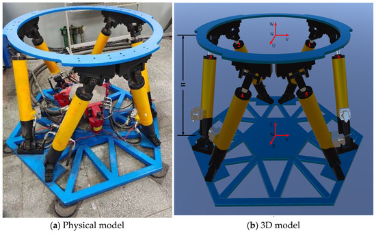
Figure 1.
The electro-hydraulic Stewart parallel mechanism.
The motion state of the parallel mechanism can be determined through inverse kinematics solutions, whereby the displacements of the six hydraulic cylinders in the electro-hydraulic Stewart parallel mechanism are calculated based on its given position and orientation.
The origin N of coordinate system N is represented in coordinate system M as a three-dimensional vector, denoted by
where
denotes the projection position of the origin
of coordinate system N onto the X-axis in coordinate system M;
and
follow the same definition;
represents the vertical distance between the centers of the fixed platform and moving platform in the initial state.
The translation matrix from coordinate system M to coordinate system N is
when the moving platform rotates to a specific orientation, the Euler angles in three orthogonal directions uniquely define a rotation matrix. Through coordinate transformation, the absolute position of the moving platform can be determined. The resulting rotation matrix
is expressed as
where
,
and
denote the rotation angles of the moving platform coordinate system N about the Z-axis, Y-axis, and X-axis of the fixed platform coordinate system M, respectively;
,
and
represent the rotation matrices of the moving platform coordinate system N about the Z-axis, Y-axis, and X-axis of the fixed platform coordinate system M, respectively.
The pose matrix P of the moving platform coordinate system N is expressed as
The schematic top view of the Electro-Hydraulic Stewart parallel mechanism is shown in Figure 2. Here,
(where
) denotes the three-dimensional column vectors representing the positional vectors of the six hinge points on the fixed platform along the X-, Y-, and Z-axes in the fixed platform coordinate system M. Similarly,
represents the three-dimensional column vectors describing the positional vectors of the six hinge points on the moving platform along the X-, Y-, and Z-axes in the moving platform coordinate system N.
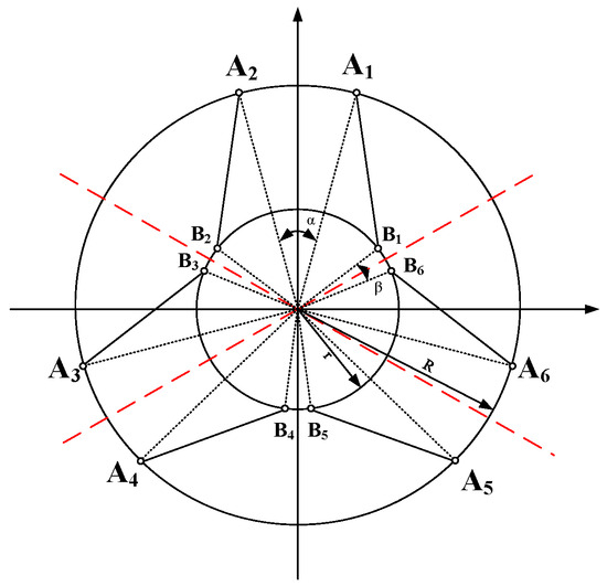
Figure 2.
Schematic top view of the electro-hydraulic Stewart parallel mechanism.
The coordinates of the six hinge points on the fixed platform in coordinate system M can be represented by a 3 × 6 matrix A:
The coordinates of the six hinge points at the initial position of the moving platform in coordinate system N can be represented by a 3 × 6 matrix B:
where α denotes the angle between two adjacent hinge points on the fixed platform at the origin of coordinate system M; β represents the angle between two adjacent hinge points on the moving platform at the origin of coordinate system N; R is the radius of the fixed platform; r is the radius of the moving platform; c and s denote cosine (cos) and sine (sin), respectively.
After being transformed by the pose matrix P, the six hinge points on the moving platform coordinate system N are expressed in the fixed platform coordinate system M as
where
denotes the coordinates of the six hinge points in the moving platform coordinate system N after transformation into the fixed platform coordinate system M.
From Equation (7), we have
where
denotes the initial length of the i-th hydraulic cylinder in the initial state;
represents the length of the i-th hydraulic cylinder after the transformation of the moving platform coordinate system N by the pose matrix P;
indicates the displacement of the piston rod for the i-th hydraulic cylinder.
2.2. Dynamic Analysis
Let
denote the center of gravity position of the moving platform in the moving coordinate system. Then, the center of gravity position
of the moving platform in the fixed coordinate system can be expressed as
The acceleration
of the center of gravity of the moving platform is:
where
denotes the angular acceleration at the origin of the moving platform;
represents the angular velocity of the moving platform;
is the distance from the origin M of the fixed platform to the origin N of the moving platform;
signifies the linear acceleration at the origin of the moving platform.
Let
denote the moment of inertia of the moving platform with respect to the moving coordinate system. Then, the moment of inertia
of the moving platform with respect to the fixed coordinate system can be expressed as
Performing force analysis on the moving platform, according to Newton’s equations, we have
In the equations: M is the mass of the moving platform;
denotes the external load force acting on the moving platform;
represents the constraint force exerted by the i-th Hooke joint on the moving platform.
For the moving platform, the frictional torque induced by the upper Hooke joint is given by
where
is the viscous friction coefficient of the Hooke joint;
is the angular velocity of the actuator leg.
Applying Euler’s equations to the moving platform yields the expression:
In the equations:
denotes the external torque acting on the moving platform,
defines the parameter
in the fixed coordinate system M.
By combining Equations (12)–(14) and (16), the compact form of the dynamic model for the entire electro-hydraulic Stewart platform can be derived.
where
is the generalized inertia matrix;
denotes the angular acceleration of the moving platform;
represents the nonlinear coupling term;
is the force mapping matrix;
signifies the output forces of the six hydraulic legs.
3. DDPG Algorithm Model
The DDPG algorithm comprises two neural networks: the Actor and the Critic. The Actor generates deterministic actions, while the Critic evaluates the value of state-action pairs. When dealing with multiple action outputs, the Actor network typically includes multiple output nodes, each corresponding to a distinct action dimension. However, if these actions exhibit coupling relationships—for instance, certain actions cannot simultaneously reach maximum values or must satisfy specific constraints—simple independent output mechanisms may prove insufficient. DDPG addresses these challenges through trial-and-error learning of environmental dynamics, including coupling effects. Provided the observation space contains sufficient information and the Critic network is sufficiently robust, the agent can autonomously learn these interdependent constraints. The control framework of the DDPG agent (RL agent) is illustrated in Figure 3.
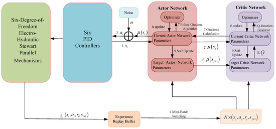
Figure 3.
DDPG-PID control framework.
As shown in Figure 3,
is the i-th output action,
is the i-th input state,
is the i-th reward,
is the i-th action without noise, Q is the evaluation value. The RL agent module employs a 24-dimensional observation space consisting of six hydraulic cylinder piston rod displacements, six deviations between the desired displacements and actual displacements, six integrals of these deviations, and six control currents of the electro-hydraulic proportional valves. The action space is defined as 18-dimensional, corresponding to the proportional, integral, and derivative gains of six PID controllers. To address the coupling effects among the six degrees of freedom, the agent implements global data standardization protocols for both observations and actions.
The termination condition (isdone function) specifies when the system should terminate. The system is terminated and deemed invalid if the piston rod displacement exceeds
or falls below 0. The isdone function is defined in Equation (18):
where
denotes the extension length (in meters) of the piston rod in the i-th (i = 1,2, …, 6) hydraulic cylinder;
represents the logical OR operation.
The reward function is designed to balance tracking accuracy and training energy consumption, comprising the following components: Position Error Term, Maximum Position Error Penalty Term, Error Coupling Suppression Term and Over-Travel Penalty Term. The total reward is given by Equation (18):
In the DDPG algorithm, determining the coefficients of the reward function is a critical factor influencing training success, yet no unified mathematical formula exists. This paper primarily employs experimental parameter tuning to establish expressions
,
,
and
. The reward function comprises the following terms:
- Position Error Term:where represents the position error of the i-th (i = 1,2,…,6) hydraulic cylinder, and is the position error weighting coefficient.
- Maximum Position Error Penalty Term:where denotes the maximum value of the squared position error of the i-th (i = 1,2,…,6) hydraulic cylinder, and is the maximum position error penalty weighting coefficient, .
- Error Coupling Suppression Term:where and ( = 1,2,…,6, = 2,…,6, < ) are the position errors of two distinct hydraulic cylinders, and is the error coupling suppression weighting coefficient
- Over-Travel Penalty Term:
The piston rod displacement of the hydraulic cylinder is constrained to
, and penalties are imposed if this range is violated, with
acting as the over-travel penalty weighting coefficient,
.
In designing the reward function, since deviations may be positive or negative, rewards or penalties are applied based on the squared deviation and its maximum value. A positive coefficient corresponds to a reward, while a negative coefficient indicates a penalty. The absolute value of the product of errors from two degrees of freedom is used as a coupling suppression term, with a threshold set such that exceeding it incurs a penalty, while staying below it yields a reward.
4. Comparative Experimental Analysis
4.1. Simulation Environment Setup
The schematic diagrams of the DDPG-PID control and PID control principles for the electro-hydraulic Stewart parallel mechanism are shown in Figure 4.
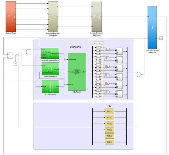
Figure 4.
Schematic diagrams of DDPG-PID control and PID control for the electro-hydraulic Stewart parallel mechanism.
By modifying the desired pose input
of the moving platform in Figure 4, the inverse kinematic model can adjust the desired piston rod displacements of the hydraulic cylinders. This enables precise control of the six hydraulic cylinder piston rod displacements based on the desired pose of the moving platform. After normalization in DDPG, the action output range is [−1, 1]. After scaling module adjustment, the proportional gain range is [5000, 11,000], integral gain is [0, 800], derivative gain is [0, 400]. The Actor and Critic network structures created by the DDPG algorithm in this paper are shown in Figure 5. Since both DDPG-PID and PID employ unity feedback, the position error equals the deviation signal input to the controller. The primary physical parameters of the electro-hydraulic Stewart parallel mechanism are listed in Table 1.
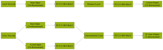
Figure 5.
Network structure diagram of Actor and Critic created by DDPG algorithm.

Table 1.
Key physical parameters of the electro-hydraulic Stewart.
The Actor and Critic network structures created by the DDPG algorithm in this paper are shown in Figure 5.
As shown in Figure 5, FC512 denotes Fully Connected Layer (512 neurons), BN denotes Batch Normalization, ReLU denotes Rectified Linear Unit. The output action uses the tanh (hyperbolic tangent) function for normalization, thus limiting the output value range to [−1, 1].
The key parameters of the agents are listed in Table 2.
Table 2.
The key parameters of the agents.
4.2. Comparative Experiment
Under identical desired moving platform pose inputs
, comparative motion control experiments were conducted on the electro-hydraulic Stewart parallel mechanism using both traditional PID and DDPG-PID algorithms. Identical sinusoidal signals with varying amplitudes and frequencies were applied to each desired pose input
. The inverse kinematic model then generated the desired elongation values for the six hydraulic cylinder piston rods.
After implementing control via deep reinforcement learning DDPG-PID and PID on the electro-hydraulic Stewart parallel mechanism, the position error exhibited an approximately sinusoidal curve. Positive values indicate the actual value is less than the desired value, while negative values indicate the actual value exceeds the desired value.
The hardware platform configuration adopted in this paper is as follows: Intel i5 12600KF processor (10 cores), 32 GB of DDR5 RAM, and an NVIDIA GeForce RTX 4070 Ti GPU (16 GB VRAM). A single model training process requires approximately 4 to 5 h.
Experiments involved generating linear displacement (x, y, z) and angular displacement (φ, γ, θ) signals with varying amplitudes and frequencies, corresponding to the extension/retraction motions of the six hydraulic cylinders in the parallel mechanism. All hydraulic cylinder strokes were strictly constrained within the range of [0,0.3] m. To ensure robustness and practicality during training, amplitude and frequency settings of input signals incorporated safety margins. Preliminary testing revealed that certain input combinations caused cylinder stroke overlimits or poor identifiability; for example: with linear displacement 0.03sin(0.15πt) m and angular displacement 8.93sin(0.15πt)°, one hydraulic cylinder exceeded its stroke limit while two cylinders exhibited only positive half-cycle sinusoidal motion and another showed only negative half-cycle motion, indicating incomplete motion patterns; with linear displacement 0.09sin(0.525πt) m and angular displacement 4.01sin(0.525πt)°, one cylinder similarly exceeded its stroke limit; with linear displacement 0.03sin(0.15πt) m and angular displacement 3.44sin(0.525πt)°, all six cylinders demonstrated low trajectory identifiability and poor readability. Considering these factors comprehensively—stroke constraints, motion completeness, trajectory discernibility, and the need to clearly demonstrate system coupling characteristics and controller performance—this study ultimately selected two representative input signals for analysis: a low-frequency/low-amplitude signal (linear displacement 0.03sin(0.15πt) m, angular displacement 1.72sin(0.15πt)°) and a high-frequency/high-amplitude signal (linear displacement 0.06sin(0.525πt) m, angular displacement 3.44sin(0.525πt)°).
- Input signals: linear displacement 0.03sin(0.15πt) m, angular displacement 1.72sin(0.15πt)°
Under the PID control algorithm, the input signals, desired vs. actual piston rod displacements of the hydraulic cylinders, and position errors are illustrated in Figure 6a–c, respectively. The proportional, integral, and derivative gains of the six PID controllers are fixed and identical, as shown in Figure 7.
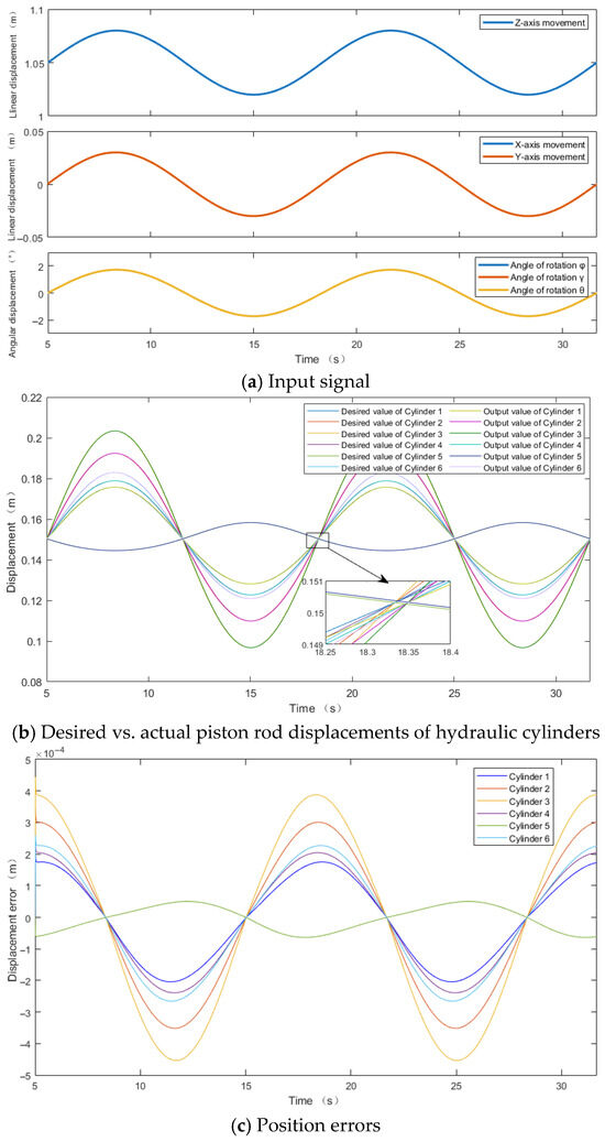
Figure 6.
PID control algorithm.
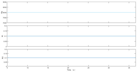
Figure 7.
PID Control gains.
For the DDPG-PID control algorithm, the corresponding input signals, desired vs. actual piston rod displacements, and position errors are shown in Figure 8a–c. The proportional, integral, and derivative gains of the six PID controllers are dynamically adjusted by DDPG, as shown in Figure 9.
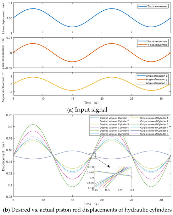
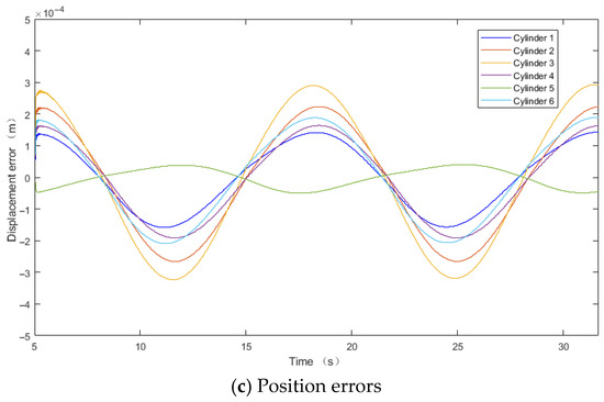
Figure 8.
DDPG-PID control algorithm.
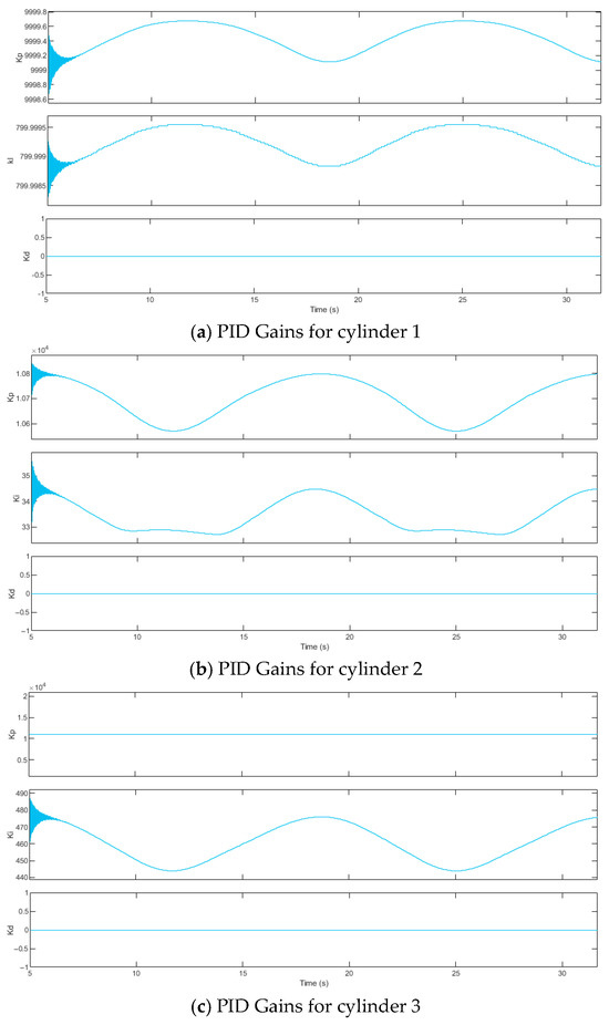
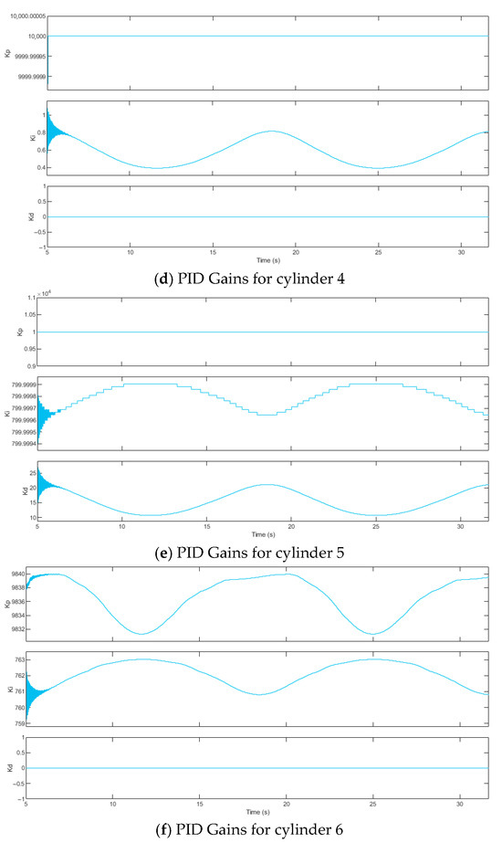
Figure 9.
DDPG-PID Control Gains.
Considering that the piston rods of all six hydraulic cylinders do not exceed the upper stroke limit (0.3 m) or lower stroke limit (0 m) during operation, within the 0~5 s time period, a constant input signal of
= 0.9 + 0.15 = 1.05 m is applied to the z-axis, raising the moving platform to the mid-position. According to Figure 6a and Figure 8a, under both control algorithms, linear displacement with an amplitude of 0.03 m and angular frequency of 0.15π rad/s are input to (x, y, z), angular displacement with an amplitude of 1.72° and angular frequency of 0.15π rad/s are input to (φ, γ, θ). The input signals for x and y are identical, coinciding as a single curve. And the input signals for φ, γ, and θ are identical, coinciding as a single curve.
According to Figure 6b and Figure 8b, at the mid-position, the initial elongation values for all six hydraulic cylinders are 0.15 m, with a motion period of 13.33 s. Cylinder 3 exhibits the largest action range, with a maximum desired elongation of 0.2034 m and a minimum desired elongation of 0.0968 m.
A comparison of Figure 6c and Figure 8c reveals significant improvements in position errors, where the maximum peak errors under the PID control algorithm are 0.00039 m and −0.00045 m, while under the DDPG-PID control algorithm, they are 0.00029 m and −0.00032 m, respectively.
The maximum errors for the six hydraulic cylinders are reduced as follows: from −0.00020 m, 0.00030 m, −0.00045 m, −0.00024 m, 0.00005 m, −0.00027 m to −0.00016 m, 0.00023 m, −0.00032 m, −0.00019 m, 0.00004 m, −0.00021 m
The maximum position error reductions are 20.00%, 23.33%, −28.89%, 20.83%, 20%, and 22.22%, respectively, clearly demonstrating the superiority of the DDPG-PID control strategy over traditional PID control.
Comparing Figure 7 and Figure 9: Under the PID control algorithm, the proportional gain kp, integral gain ki, and derivative gain kd fixed at 8000, 0.1, and 0.1, respectively. The proportional gain is tuned using the Ziegler-Nichols method, while the integral and derivative gains are subsequently determined through experimental parameter tuning based on the established proportional gain. Under the DDPG-PID control algorithm: For Cylinder 1: kp adjusts within [9998.68, 9999.68] in a standard sinusoidal waveform; ki adjusts within [799.998, 799.999] in a non-standard sinusoidal waveform; kd = 0. For Cylinder 2: kp adjusts within [10,570, 10,840] in a standard sinusoidal waveform; ki adjusts within [32.71,35.56] in a non-standard sinusoidal waveform; kd = 0. For Cylinder 3: kp is fixed at 11,000; ki adjusts within [444,486.9] in a standard sinusoidal waveform; kd = 0. For Cylinder 4: kp is fixed at 10,000; ki adjusts within [0.39, 1.08] in a standard sinusoidal waveform; kd = 0. For Cylinder 5: kp is fixed at 10,000; ki adjusts within [799.9994, 799.9999] in a non-standard sinusoidal waveform; kd adjusts within [10.68, 27.08] in a standard sinusoidal waveform. For Cylinder 6: kp adjusts within [9831, 9840] in a non-standard sinusoidal waveform; ki adjusts within [759.3, 763] in a standard sinusoidal waveform; kd = 0. The derivative terms of the PID controllers for Cylinders 1, 2, 3, 4, and 6 have no adjustment function, essentially functioning as PI controllers.
- 2.
- Input signals: linear displacement 0.06sin(0.525πt) m, angular displacement 3.44sin(0.525πt)°
Under the PID control algorithm, the input signals, desired vs. actual piston rod displacements of the hydraulic cylinders, and position errors are illustrated in Figure 10a–c, respectively. The proportional, integral, and derivative gains of the six PID controllers are essentially consistent with those shown in Figure 7.
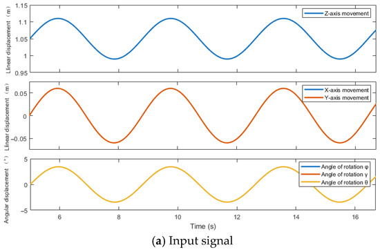
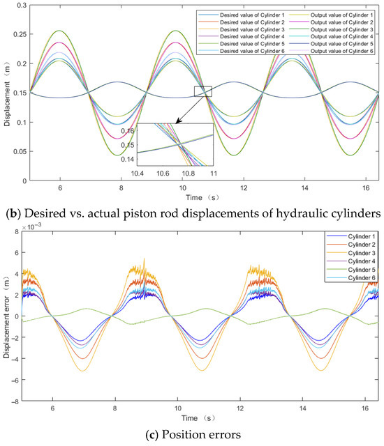
Figure 10.
PID control algorithm.
For the DDPG-PID control algorithm, the corresponding input signals, desired vs. actual piston rod displacements, and position errors are shown in Figure 11a–c. The proportional, integral, and derivative gains of the six PID controllers are dynamically adjusted by DDPG, as shown in Figure 12.
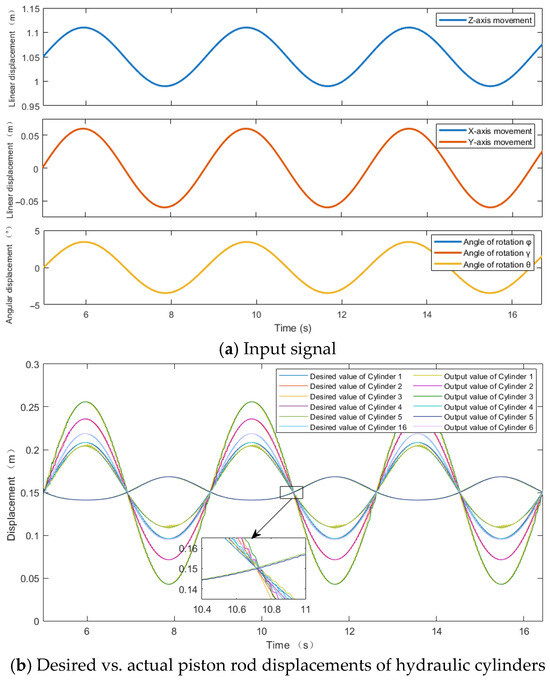
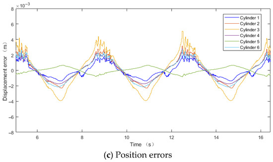
Figure 11.
DDPG-PID control algorithm.
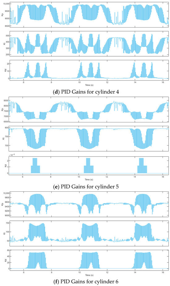
Figure 12.
DDPG-PID Control Gains.
The desired pose inputs
are sinusoidal signals with an amplitude of 0.06 m and angular frequency 0.525π rad/s. And the desired pose inputs
are sinusoidal signals with an amplitude of 3.44° and angular frequency 0.525π rad/s. Through the inverse kinematic sub-model, the desired displacements for the six hydraulic cylinders are calculated. As shown in Figure 10b and Figure 11b, the six hydraulic cylinders exhibit a consistent motion period of 3.81 s. Among them, Cylinder 3 demonstrates the largest displacement range, with a maximum desired extension of 0.2559 m and a minimum desired extension of 0.0429 m.
Under the PID control algorithm, the proportional gain kp, integral gain ki, and derivative gain kd remain fixed at 8000, 0.1, and 0.1, respectively, as shown in Figure 7. Under the DDPG-PID control algorithm: for Cylinder 1, kp, ki, and kd dynamically adjust within [9051, 10,000], [53.6,548.3], and [0.00035, 74.2], respectively; for Cylinder 2, kp, ki, and kd dynamically adjust within [8075, 10,980], [367.2, 742.9], and [6.75, 48.99], respectively; for Cylinder 3, kp, ki, and kd dynamically adjust within [9571, 10,580], [154.5,366.4], and [0.00024, 38.8], respectively; for Cylinder 4, kp, ki, and kd dynamically adjust within [8579, 9946], [211.2, 529.8], and [0.00041, 22.25], respectively; for Cylinder 5, kp, ki, and kd dynamically adjust within [6664, 8520], [681.4, 795], and [0, 0.000024], respectively; for Cylinder 6, kp, ki, and kd dynamically adjust within [9038, 9959], [38.82, 147.9], and [0.00006, 54.25], respectively.
Comparing Figure 9 and Figure 12, for input signals of linear displacement 0.06sin(0.525πt) m and angular displacement 3.44sin(0.525πt)°, the training process of DDPG-PID control is more complex than for linear displacement 0.03sin(0.15πt) m and angular displacement 1.72sin(0.15πt)°. The variation curve of the DDPG agent’s reward with training episodes is shown in Figure 13.
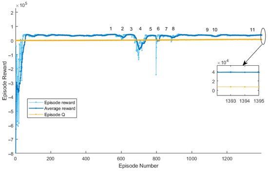
Figure 13.
DDPG Agent Reward Variation Curve with Training Episodes.
As seen in Figure 13, the initial episode reward is approximately −8 ×
. After training commences, both episode reward and average reward increase exponentially. At episode 66, the episode reward and average reward nearly converge, while the evaluation value Q steadily increases. The agent attains local optima in regions 1, 3, 5, 7, and 9. When attempting to further reduce tracking error in one or several degrees of freedom of the Stewart parallel mechanism, strong coupling among the six DoFs causes tracking errors in other DoFs to worsen or even severely deteriorate, leading to declines in episode and average rewards. After further exploration of intrinsic relationships among the six DoFs, rewards rise rapidly in regions 2, 4, 6, 8, and 10. During these phases, Q steadily increases, indicating effective learning strategies. In region 11, episode and average rewards converge and fluctuate slightly around 40,000 without significant upward trends, suggesting the control strategy has likely found or approached the global optimum. Training concludes at episode 1395. The reward curves fully reflect the strong coupling of the Stewart parallel mechanism and the intelligence of the DDPG agent.
According to Figure 10c and Figure 11c, significant pulsation occurs at the mid-position intersection of the six hydraulic cylinders. This is primarily because, in this working region, the acceleration of the six hydraulic cylinder piston rods exhibits substantial abrupt changes with varying magnitudes. Taking Cylinder 3 as an example, the acceleration of the displacement deviation signal is shown in Figure 14.
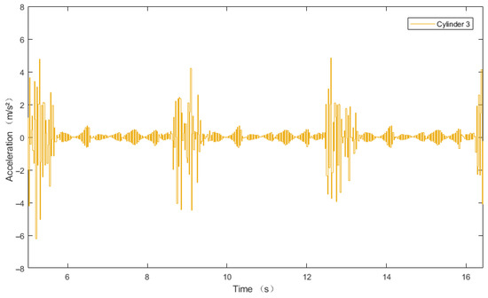
Figure 14.
DDPG-PID Acceleration curve diagram of displacement deviation signal for cylinder 3.
According to Figure 14, near 12.6 s (mid-position intersection), the acceleration of the displacement deviation signal in this working region reaches a maximum of 4.849 m/s2 and a minimum of −3.936 m/s2, demonstrating strong nonlinear characteristics.
The change in acceleration causes a change in velocity. The velocity of the displacement deviation signal is shown in Figure 15.
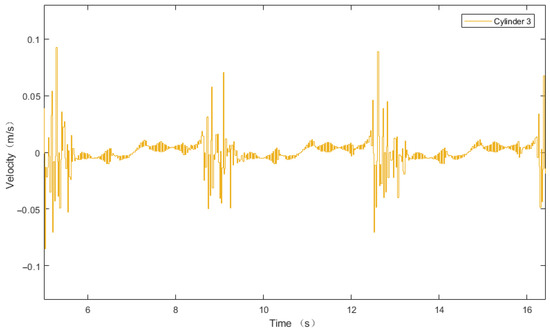
Figure 15.
DDPG-PID Velocity curve diagram of displacement deviation signal for cylinder 3.
In Figure 11b, the slope of the desired versus actual elongation curves of the hydraulic cylinder piston rods represents velocity. If the slopes are identical, the velocity of the displacement deviation signal is zero, indicating smooth curves. A larger absolute value of the displacement deviation signal’s velocity implies greater pulsation of the actual piston rod elongation compared to the desired value. According to Figure 15, near 12.6 s in the working region, the maximum velocity is 0.089 m/s and the minimum velocity is −0.070 m/s.
Hydraulic systems are inherently time-delay systems, meaning there is a lag between the current control signal and the hydraulic cylinder’s motion response. When the DDPG policy outputs high-acceleration commands, the hydraulic actuator must overcome greater inertial forces. If the system’s driving force is insufficient or the response is delayed, tracking errors accumulate. These velocity changes ultimately result in flow pulsations in the rod-side chamber of the hydraulic cylinder, as shown in Figure 16.
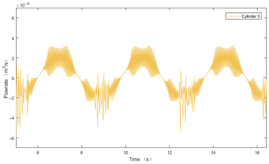
Figure 16.
DDPG-PID cylinder 3 flow pulsation curve graph.
Figure 16 demonstrates significant flow pulsation in this region, with a maximum of 0.00007 m3/s and a minimum of −0.00044 m3/s, further confirming strong nonlinear behavior. The rapidity and smoothness of trajectory tracking are inherently conflicting objectives. Improving tracking precision necessitates higher rapidity, which manifests as large abrupt changes in hydraulic cylinder piston rod acceleration. This ultimately induces pulsations in the actual piston rod displacement within this operational range.
A comparison of Figure 10c and Figure 11c reveals significant improvements in position errors, where the maximum peak errors under the PID control algorithm are 0.0049 m and −0.0053 m, while under the DDPG-PID control algorithm, they are 0.0050 m and −0.0039 m, respectively.
The maximum errors for the six hydraulic cylinders are reduced as follows: from −0.00233 m, −0.00414 m, −0.00532 m, −0.00278 m, 0.00081 m, −0.00305 m to −0.00136 m, −0.00230 m, −0.00391 m, −0.00172 m, 0.00065 m, −0.00215 m
The maximum position error reductions are 41.63%, 44.44%, 26.50%, 38.13%, 19.75%, and 29.51%, respectively.
In traditional PID control, the proportional, integral, and derivative gains remain fixed. At an input signal of linear displacement 0.03sin(0.15πt) m and angular displacement 1.74sin(0.15πt)°, the position errors reach micrometer-level magnitudes. However, with an input signal of linear displacement 0.06sin(0.525πt) m and angular displacement 3.44sin(0.525πt)°, the position errors become larger. After training the proportional, integral, and derivative gains via the reinforcement learning agent, the DDPG-PID control outperforms traditional PID control under both input signal conditions.
5. Conclusions
The operating condition with simultaneous amplitude and frequency variations in each degree of freedom of the electro-hydraulic Stewart parallel mechanism represents the most common working scenario. However, due to mutual influences among the six degrees of freedom, the coupling and nonlinearity are also most complex in this case. This paper adopts a hybrid DDPG and PID control approach to fully leverage the complementary advantages of both algorithms. For an input signal of linear displacement 0.03sin(0.15πt) m and angular displacement 1.74sin(0.15πt)°, the maximum trajectory tracking error is reduced by 28.89%; for an input signal of linear displacement 0.06sin(0.525πt) m and angular displacement 3.44sin(0.525πt)°, the maximum trajectory tracking error is reduced by 44.44%, achieving adaptive high-precision trajectory tracking control objectives. The following conclusions can be drawn:
- (1)
- For traditional PID control algorithms, control parameters rely on prior knowledge for design. Fixed control parameters struggle to adapt to dynamic changes, requiring frequent manual tuning. Each controller operates independently without information-sharing mechanisms, unable to proactively explore new operating conditions. Some improved algorithms based on this, such as Fuzzy+PID, Neural Network+PID, and feedforward-feedback control, exhibit limited practical control performance for high-order, strongly coupled, highly nonlinear systems like the electro-hydraulic Stewart parallel mechanism. This limitation stems from issues like high computational load, insufficient real-time capability, and difficulties in establishing precise models.
- (2)
- Deep reinforcement learning agents directly learn nonlinear mapping relationships, perceive environmental changes (e.g., load transients, disturbances) in real-time, autonomously adjust strategies dynamically, and proactively address issues like multivariable coupling, disturbance rejection, and fault tolerance. However, no control algorithm is perfect: Compared to PID control, DDPG-PID achieves higher control accuracy through real-time dynamic adjustment of control gains, but exhibits inferior smoothness in trajectory tracking curves. In the DDPG algorithm, observation range, action range, learning rate, noise intensity, and reward function gains collectively affect training stability, convergence speed, and final performance, requiring timely adjustments during training. The DDPG algorithm imposes high computational demands; for the complex operating condition discussed in this paper—synchronous variable-amplitude variable-frequency sinusoidal excitation across all 6 degrees of freedom—hardware configuration directly impacts training speed, algorithm stability, and experimental efficiency.
Author Contributions
Conceptualization, Y.K. and Y.W. (Yulong Wang); methodology, Y.K. and Y.W. (Yulong Wang); writing—original draft, Y.K. and Y.W. (Yulong Wang); formal analysis, Y.W. (Yueran Wang) and S.Z.; investigation, Y.K. and R.Z.; project administration, Y.K.; software, Y.W. (Yulong Wang), Y.W. (Yueran Wang) and S.Z.; supervision, Y.K.; validation, R.Z. and L.W.; writing—review and editing, Y.K. and Y.W. (Yulong Wang). All authors have read and agreed to the published version of the manuscript.
Funding
This paper was financially supported by the Shanxi Provincial New Energy Aviation Intelligent Support Equipment Technology Innovation Center and the Basic Research Program Project of Shanxi Province, China (no. 202403021211077).
Data Availability Statement
The original contributions presented in this study are included in the article. The data used to support the findings of this study are available from the corresponding authors.
Conflicts of Interest
Author Yueran Wang was employed by the company North Navigation Control Technology Co., Ltd. The remaining authors declare that the research was conducted in the absence of any commercial or financial relationships that could be construed as a potential conflict of interest.
References
- Furqan, M.; Suhaib, M.; Ahmad, N. Studies on Stewart platform manipulator: A review. J. Mech. Sci. Technol. 2017, 31, 4459–4470. [Google Scholar] [CrossRef]
- McCann, C.; Patel, V.; Dollar, A. The Stewart Hand. IEEE Robot. Autom. Mag. 2021, 28, 23–36. [Google Scholar] [CrossRef]
- Bi, F.; Ma, T.; Wang, X.; Yang, X.; Lv, Z. Research on Vibration Control of Seating System Platform Based on the Cubic Stewart Parallel Mechanism. IEEE Access 2019, 7, 155637–155649. [Google Scholar] [CrossRef]
- Karmakar, S.; Turner, C.J. A Literature Review on Stewart-Gough Platform Calibrations. J. Mech. Des. 2024, 146, 083302. [Google Scholar] [CrossRef]
- Kazezkhan, G.; Xu, Q.; Wang, N.; Xue, F.; Wang, H. Performance Analysis and Optimization of a Modified Stewart Platform for the Qitai Radio Telescope. Res. Astron. Astrophys. 2023, 23, 095022. [Google Scholar] [CrossRef]
- Ma, T.; Li, T.J.; Jing, G.X.; Liu, H.; Bi, F.R. Development of a Novel Seat Suspension Based on the Cubic Stewart Parallel Mechanism and Magnetorheological Fluid Damper. Appl. Sci. 2022, 12, 11437. [Google Scholar] [CrossRef]
- Peterson, T.R. Design and Implementation of Stewart Platform Robot for Robotics Course Laboratory. Master’s Thesis, California Polytechnic State University, San Luis Obispo, CA, USA, 2020. [Google Scholar]
- Tang, J.; Cao, D.Q.; Yu, T.H. Decentralized vibration control of a voice coil motor-based Stewart parallel mechanism: Simulation and experiments. Proc. Inst. Mech. Eng. Part C J. Mech. Eng. Sci. 2019, 233, 132–145. [Google Scholar] [CrossRef]
- Wang, Z.J.; Yang, C.H.; Che, R.Q.; Li, H.X.; Chen, Y.P.; Chen, L.J.; Yuan, W.X.; Yang, F.; Tian, J.; Wang, B.J. Assisted Tea Leaf Picking: The Design and Simulation of a 6-DOF Stewart Parallel Lifting Platform. Agronomy 2024, 14, 844. [Google Scholar] [CrossRef]
- Tian, T.; Jiang, H.; Tong, Z.; He, J.; Huang, Q. An inertial parameter identification method of eliminating system damping effect for a six-degree-of-freedom parallel manipulator. Chin. J. Aeronaut. 2015, 28, 582–592. [Google Scholar] [CrossRef]
- Jishnu, A.K.; Chauhan, D.K.; Vundavilli, P.R. Design of neural network-based adaptive inverse dynamics controller for motion control of stewart platform. Int. J. Comput. Methods 2022, 19, 2142010. [Google Scholar] [CrossRef]
- Phan, V.D.; Vo, C.P.; Ahn, K.K. Adaptive neural tracking control for flexible joint robot including hydraulic actuator dynamics with disturbance observer. Int. J. Robust Nonlinear Control 2024, 34, 8744–8767. [Google Scholar] [CrossRef]
- Phan, V.D.; Phan, Q.C.; Ahn, K.K. Observer-Based Adaptive Fuzzy Tracking Control for a Valve-Controlled Electro-Hydraulic System in Presence of Input Dead Zone and Internal Leakage Fault. Int. J. Fuzzy Syst. 2025. [Google Scholar] [CrossRef]
- Cai, W.; Zhang, Y.; Zhang, J.; Guo, S.; Guo, R. Prediction of Input–Output Characteristic Curves of Hydraulic Cylinders Based on Three-Layer BP Neural Network. Sensors 2025, 25, 1949. [Google Scholar] [CrossRef]
- Liu, N.; Chai, T.; Zhang, Y.; Gao, W. Data-driven optimal tuning of PID controller parameters. Sci. China-Inf. Sci. 2025, 68, 172201:1–172201:21. [Google Scholar] [CrossRef]
- Omurlu, V.E.; Yildiz, I. Parallel self-tuning fuzzy PD+ PD controller for a Stewart–Gough platform-based spatial joystick. Arab. J. Sci. Eng. 2012, 37, 2089–2102. [Google Scholar] [CrossRef]
- Taghizadeh, M.; Javad Yarmohammadi, M. Development of a self-tuning PID controller on hydraulically actuated stewart platform stabilizer with base excitation. Int. J. Control Autom. Syst. 2018, 16, 2990–2999. [Google Scholar] [CrossRef]
- Barghandan, M.; Pirmohamadi, A.A.; Mobayen, S.; Fekih, A. Optimal adaptive barrier-function super-twisting nonlinear global sliding mode scheme for trajectory tracking of parallel robots. Heliyon 2023, 9, e13378. [Google Scholar] [CrossRef]
- Shahbazi, M.; Heidari, M.; Ahmadzadeh, M. Optimization of dynamic parameter design of Stewart platform with Particle Swarm Optimization (PSO) algorithm. Adv. Mech. Eng. 2024, 16, 1–16. [Google Scholar] [CrossRef]
- Zhao, D.; Li, S.; Gao, F. Fully adaptive feedforward feedback synchronized tracking control for Stewart Platform systems. Int. J. Control Autom. Syst. 2008, 6, 689–701. [Google Scholar]
- Cai, Y.; Zheng, S.; Liu, W.; Qu, Z.; Han, J. Model analysis and modified control method of ship-mounted Stewart platforms for wave compensation. IEEE Access 2021, 9, 4505–4517. [Google Scholar] [CrossRef]
- Dong, Z.; He, S.; Liao, Y.; Wang, H.; Song, M.; Jiang, J.; Chen, G. Pressure Control in the Pump-Controlled Hydraulic Die Cushion Pressure-Building Phase Using Enhanced Model Predictive Control with Extended State Observer-Genetic Algorithm Optimization. Actuators 2025, 14, 261. [Google Scholar] [CrossRef]
- Mirza, M.A.; Li, S.; Jin, L. Simultaneous learning and control of parallel Stewart platforms with unknown parameters. Neurocomputing 2017, 266, 114–122. [Google Scholar] [CrossRef]
- Shi, Y.; Sheng, W.; Wang, J.; Jin, L.; Li, B.; Sun, X. Real-time tracking control and efficiency analyses for Stewart platform based on discrete-time recurrent neural network. IEEE Trans. Syst. Man Cybern. Syst. 2024, 54, 5099–5111. [Google Scholar] [CrossRef]
- Jiang, Z.; Chen, Z.; Xu, K.; Shi, L. Distributed collaborative control to pose tracking for six-DOF parallel mechanism under multi-cylinder communication. ISA Trans. 2025, 159, 312–325. [Google Scholar] [CrossRef]
- Huang, H.C.; Chen, Y.X. Evolutionary optimization of fuzzy reinforcement learning and its application to time-varying tracking control of industrial parallel robotic manipulators. IEEE Trans. Ind. Inform. 2023, 19, 11712–11720. [Google Scholar] [CrossRef]
- Han, R.; He, H.; Wang, Y.; Wang, Y. Reinforcement Learning Based Energy Management Strategy for Fuel Cell Hybrid Electric Vehicles. Chin. J. Mech. Eng. 2025, 38, 66. [Google Scholar] [CrossRef]
- Huang, H.C.; Xu, S.S.D.; Chen, Y.X.; Chen, C.M. Reinforcement Fuzzy Q-Learning Incorporated with Genetic Kinematics Analysis for Self-organizing Holonomic Motion Control of Six-Link Stewart Platforms. Int. J. Fuzzy Syst. 2023, 25, 1239–1255. [Google Scholar] [CrossRef]
- Yadavari, H.; Tavakol Aghaei, V.; İkizoğlu, S. Deep reinforcement learning-based control of Stewart platform with parametric simulation in ROS and Gazebo. J. Mech. Robot. 2023, 15, 035001:1–035001:11. [Google Scholar] [CrossRef]
- Wang, W.; Zhang, X.; Han, L.L.; Wang, M.; Zhong, Y.B. Inverse kinematics analysis of 6-DOF Stewart platform based on homogeneous coordinate transformation. Ferroelectrics 2018, 522, 108–121. [Google Scholar] [CrossRef]
- Li, Z. Virtual Experimental Teaching Platform for Hydraulic Six-DOF Parallel Mechanism Based on UDP Communication Technology. Master’s Thesis, Taiyuan University of Science and Technology, Taiyuan, China, 2023. [Google Scholar] [CrossRef]
- Wang, Y.; Kong, Y.; Li, Z.; Zhang, H.; Li, C.; Wang, X. Virtual Reality Technology of Hydraulic Six-DOF Parallel Mechanism Driven by User Datagram Protocol Data. Sci. Technol. Eng. 2024, 24, 7760–7768. [Google Scholar]
- Wang, Y. Hydraulic Stewart Platform DDPG Motion Control. Master’s Thesis, Taiyuan University of Science and Technology, Taiyuan, China, 2024. [Google Scholar] [CrossRef]
Disclaimer/Publisher’s Note: The statements, opinions and data contained in all publications are solely those of the individual author(s) and contributor(s) and not of MDPI and/or the editor(s). MDPI and/or the editor(s) disclaim responsibility for any injury to people or property resulting from any ideas, methods, instructions or products referred to in the content. |
© 2025 by the authors. Licensee MDPI, Basel, Switzerland. This article is an open access article distributed under the terms and conditions of the Creative Commons Attribution (CC BY) license (https://creativecommons.org/licenses/by/4.0/).