Abstract
As the core component of aircraft systems, aeroengines require accurate Remaining Useful Life (RUL) prediction to ensure flight safety, which serves as a key part of Prognostics and Health Management (PHM). Traditional RUL prediction methods primarily fall into two main categories: physics-based and data-driven approaches. Physics-based methods mainly rely on extensive prior knowledge, limiting their scalability, while data-driven methods (including statistical analysis and machine learning) struggle with handling high-dimensional data and suboptimal modeling of multi-scale temporal dependencies. To address these challenges and enhance prediction accuracy and robustness, we propose a novel hybrid deep learning framework (CLSTM-TCN) integrating 2D Convolutional Neural Network (2D-CNN), Long Short-Term Memory (LSTM) network, and Temporal Convolutional Network (TCN) modules. The CLSTM-TCN framework follows a progressive feature refinement logic: 2D-CNN first extracts short-term local features and inter-feature interactions from input data; the LSTM network then models long-term temporal dependencies in time series to strengthen global temporal dynamics representation; and TCN ultimately captures multi-scale temporal features via dilated convolutions, overcoming the limitations of the LSTM network in long-range dependency modeling while enabling parallel computing. Validated on the NASA C-MAPSS data set (focusing on FD001), the CLSTM-TCN model achieves a root mean square error (RMSE) of 13.35 and a score function (score) of 219. Compared to the CNN-LSTM, CNN-TCN, and LSTM-TCN models, it reduces the RMSE by 27.94%, 30.79%, and 30.88%, respectively, and significantly outperforms the traditional single-model methods (e.g., standalone CNN or LSTM network). Notably, the model maintains stability across diverse operational conditions, with RMSE fluctuations capped within 15% for all test cases. Ablation studies confirm the synergistic effect of each module: removing 2D-CNN, LSTM, or TCN leads to an increase in the RMSE and score. This framework effectively handles high-dimensional data and multi-scale temporal dependencies, providing an accurate and robust solution for aeroengine RUL prediction. While current performance is validated under single operating conditions, ongoing efforts to optimize hyperparameter tuning, enhance adaptability to complex operating scenarios, and integrate uncertainty analysis will further strengthen its practical value in aircraft health management.
1. Introduction
As the critical power system, aeroengines directly determine the flight safety of aircraft through their operational status. With prolonged usage, engine systems inherently degrade over time, and even minor malfunctions may trigger catastrophic accidents. Thus, accurately assessing aeroengine health and predicting the Remaining Useful Life (RUL) are critical for ensuring stable aircraft operation and enabling proactive maintenance.
Prognostics and Health Management (PHM) serves as a comprehensive end-to-end framework that integrates detection, diagnosis, and condition forecasting, providing robust methodologies for engine health management [1]. Within PHM, RUL prediction (a classic regression task) confronts the core challenge of accurately predicting RUL from complex, high-dimensional operational parameters and dynamic degradation patterns embedded in temporal data. These operational parameters, encompassing temperature, pressure, vibration, and fuel flow, generally exhibit non-linear correlations and time-varying characteristics, while degradation processes are further influenced by multi-factors, such as operational conditions, maintenance history, and material fatigue, collectively exacerbating the complexity of RUL prediction.
Current RUL prediction methods are primarily categorized into physics-based and data-driven approaches [2], both of which enable proactive maintenance strategies to enhance the system reliability and reduce the life-cycle operational costs.
Physics-based approaches develop RUL prediction models by leveraging equipment failure and degradation mechanisms, integrated with operational parameters and condition monitoring data. These approaches require high-fidelity modeling of critical aeroengine components such as bearings, blades, hydraulic subsystems, and turbo-machinery elements. Cai et al. [3] proposed a dual non-linear recessive degradation model based on the non-linear Wiener process for RUL prediction, while Zhang et al. [4] integrated the Wiener process with evidential reasoning for complex systems. Wang et al. [5] derived a closed-form solution for the Paris–Erdogan equation to improve fatigue crack growth predictions. However, these methods rely heavily on domain expertise, limiting scalability and generality. Moreover, the real-world variability in operational environments and data uncertainty hinder their robustness [6].
In contrast, data-driven approaches directly model the degradation patterns from historical operational data to estimate RUL, mainly encompassing statistical analysis and machine learning techniques, each with unique capabilities in capturing complex degradation dynamics. Statistical approaches characterize degradation trends using probabilistic models and parameter estimation. For instance, Zhang et al. [7] applied multi-state horizontal visibility analysis to identify degradation indicators, while Peng et al. [8] utilized the takeoff exhaust gas temperature margin as a univariate RUL predictor. Gu et al. [9] improved the SbRLP method via grey Markov modeling but remained limited by the single-parameter analysis, failing to capture multi-dimensional degradation interactions.
Machine learning methods, including the auto-encoders and bidirectional Long Short-term Memory (BiLSTM) networks, excel in non-linear time series modeling. Song et al. [10] leveraged BiLSTM networks to capture bidirectional temporal dependencies for turbofan RUL prediction but faced vanishing gradients in long sequences, undermining training stability.
To address these limitations, hybrid models have emerged. Ren et al. [11] combined BiLSTM networks and Convolutional Neural Networks (CNNs) in an encoder–decoder framework for time series feature extraction and RUL prediction; Sateesh et al. [12] employed CNNs with time-dimensional convolution for aeroengine RUL prediction; Zhang et al. [13] further enhanced the accuracy of RUL prediction via multi-scale feature fusion and noise reduction, highlighting the validity of the hybrid architecture. Yu et al. [14] proposed a time series residual network to tackle sequence and feature extraction challenges, while Xu [15] developed a multi-channel SA-CNN-BILSTM model that reduced the prediction errors. Huang et al. [16] introduced a ReScConv-xLSTM predictive model to capture spatio-temporal dependencies, further improving the prediction accuracy.
Although the multi-model fusion integrates the advantages of diverse models to capture hierarchical features and complex patterns for improving accuracy and robustness, current data-driven methods still face key challenges: handling the high-dimensionality of input data, extracting effective information from multivariate time series, and modeling mixed-scale temporal dependencies.
To overcome these inherent limitations of single-model architectures and enhance the performance of aeroengine RUL prediction, we propose a novel three-layer hybrid framework (CLSTM-TCN) integrating 2D Convolutional Neural Network (2D-CNN), Long Short-Term Memory (LSTM) network, and Temporal Convolutional Network (TCN) modules: The 2D-CNN module extracts short-term local temporal features and captures inter-feature interactions, reducing high-dimensional data complexity; the LSTM module models long-term dependency in time series, enhancing the global temporal feature representation to compensate for the limitations of CNNs in long-term dependency capture; and the TCN module captures multi-scale temporal features via dilated convolutions, overcoming the LSTM network’s vanishing gradient issue in long sequences and enabling parallel computing.
Furthermore, validated on the NASA C-MAPSS data set, this framework outperforms existing hybrid models (e.g., CNN-LSTM, CNN-TCN) and single-model approaches, demonstrating superior accuracy and stability.
This paper is organized as follows: Section 2 formulates the RUL prediction problem, defines input–output relationships, and describes data characteristics. Section 3 details the theoretical foundations of core components (CNN, LSTM, and TCN) along with the CLSTM-TCN architecture and workflow. Section 4 presents the experimental design, including data preprocessing on the NASA C-MAPSS data set, evaluation metrics, and results analysis. Section 5 conducts ablation studies to validate the contribution of each module. Finally, Section 6 concludes with discussions on the study limitations and future works.
2. Problem Description
Aeroengine RUL prediction quantifies the residual operational capability during dynamic degradation, playing a critical role in ensuring flight safety and optimizing maintenance strategies. For turbofan engines (operating under extreme conditions of high temperature, pressure, and cyclic loading), RUL is defined as the maximum number of operational cycles/duration before failure. RUL is mathematically expressed as follows:
where TF(t) denotes the random failure time at the current time t, and Z(t) represents all historical information up to time t, including the sensor monitoring data, operational parameters such as the flight altitude and Mach number, and maintenance records. This definition highlights two critical characteristics impacting the complexity of aeroengine RUL prediction:
- (1)
- Conditional dependence on cumulative degradation: RUL is inherently a conditional expectation, relying on cumulative degradation information embedded in Z(t). Its accurate estimation thus depends on capturing temporal patterns in long-term monitoring data.
- (2)
- Inherent stochasticity: TF(t) is influenced by unpredictable factors such as the thermal stress-induced degradation and sensor noise. Traditional deterministic models (e.g., [4]) often oversimplify this uncertainty, leading to significant prediction errors in late-stage degradation.
2.1. Data Characteristics and Challenges
Aeroengine operational data consists of high-dimensional, multi-source time series, with diverse performance indicators recorded continuously across operational cycles. Formally, the full parameter sequence of X is an N-dimensional time series with length T:
where xt is the multivariate monitoring data at time t, and xtk∈R is the k-th sensor/parameter reading.
The NASA C-MAPSS (FD001) data set includes 24 dimensions: 3 operational settings and 21 sensors. However, 10 dimensions include static parameters (showing less than 5% variation across cycles, providing no meaningful degradation signals) and irrelevant fluctuation (oscillates randomly around zero, uncorrelated with long-term decay), which are redundant, leading to two critical challenges:
- (1)
- Computational inefficiency: 24-dimensional inputs impose higher computational burdens compared to reduced, relevant subsets (e.g., 14 dimensions).
- (2)
- Obscured critical patterns: Static noise masks subtle degradation trends in key sensors, hindering the extraction of meaningful features.
2.2. RUL Labeling and Degradation Patterns
The true RUL label sequence (Y) corresponding to X is defined as follows:
where yt ∈R is the remaining cycles until failure at time t.
Aeroengine degradation follows a non-linear two-phase pattern: a stable phase with slow performance decay (attributed to minor wear) in the first 100–150 cycles, and an accelerated phase with rapid deterioration thereafter. To align with this pattern, labels are defined using a piecewise linear function with a 125-cycle threshold [17]:
This design reduces overfitting to early-stage noise and emphasizes the late-stage trends critical for maintenance planning, addressing a key limitation of traditional single-parameter labels (e.g., [8]), which fail to capture such multi-phase dynamics.
2.3. The Prediction Task: Non-Linearity and Temporal Dependencies
The RUL prediction at time t depends on three components: the historical time series up to t − 1, prior RUL information, and current multi-source data xt:
where F(·) is an inherently non-linear function due to the complex interplay of degradation mechanisms and operational variables. Moreover, F(·) must model long-range temporal dependencies: early-cycle sensor drift can correlate with failure hundreds of cycles later.
Traditional approaches struggle to address these challenges: statistical models (such as [7]) tend to overly simplify the non-linear relationships, while individual deep learning models have distinct limitations: CNNs fail to capture long-range dependencies, LSTM networks suffer from vanishing gradients in ultra-long sequences, and TCNs alone lack fine-grained local feature extraction. This motivates our hybrid CLSTM-TCN framework, where 2D-CNN captures local feature interactions, LSTM models long-term temporal memory, and TCN complements with multi-scale dependency modeling via dilated convolutions.
In summary, our problem formulation targets the core challenges in aeroengine RUL prediction: high-dimensional redundancy, non-linear multi-phase degradation, and mixed-scale temporal dependencies, ensuring each component of the proposed framework addresses a specific aspect of the problem.
3. RUL Prediction Methods
To address the challenges of aeroengine RUL prediction, including high-dimensional data redundancy, non-linear multi-phase degradation, and mixed-scale temporal dependencies, this section reviews three core deep learning techniques (CNN, LSTM, and TCN) and introduces their integration into the hybrid CLSTM-TCN framework.
3.1. CNNs for RUL Prediction
CNNs are well-suited for aeroengine RUL prediction due to their inherent ability to capture spatio-temporal correlations in sensor data [18]. Typical CNN architecture comprises input layers, convolutional layers, pooling layers, fully connected layers, and an output layer. Convolutional layers extract local features via sliding kernels, while pooling layers reduce the dimensionality and retain the dominant features, and the fully connected layers integrate multi-scale features to generate the predicted outputs.
For aeroengine monitoring data, CNNs excel at identifying short-term local patterns and filtering noise. However, their application in RUL prediction is limited by three key drawbacks:
- (1)
- Constrained long-term dependency modeling: CNNs struggle to capture temporal relationships exceeding the kernel size, which are critical for tracking gradual degradation over hundreds of cycles.
- (2)
- Sensitivity to noise: Without robust regularization, CNNs overfit to irrelevant fluctuations in sensor data, obscuring subtle degradation trends.
- (3)
- Assumption of stationary patterns: CNNs perform poorly under varying operational conditions, where degradation dynamics shift non-linearly.
3.2. LSTM for RUL Prediction
Traditional Recurrent Neural Networks (RNNs) fail to model long-term dependencies due to vanishing/exploding gradients, but LSTM networks address this via a specialized gating mechanism that enables effective preservation of the historical information [19]. Building upon RNN frameworks, LSTM networks introduce forget, input, and output gates to regulate information flow, enabling selective retention of critical historical data while discarding noise: the forget gate determines which historical information to discard, the input gate selects new data to integrate into the memory cell, and the output gate modulates which state information is transmitted to subsequent layers, ensuring temporal consistency [20]. Complemented by a dedicated memory cell, LSTM networks preserve long-range information, which is essential for capturing imperceptible degradation trends in aeroengine sensor data. This makes them particularly effective for modeling gradual, long-term changes in engine subsystems. A schematic of the LSTM architecture is shown in Figure 1.
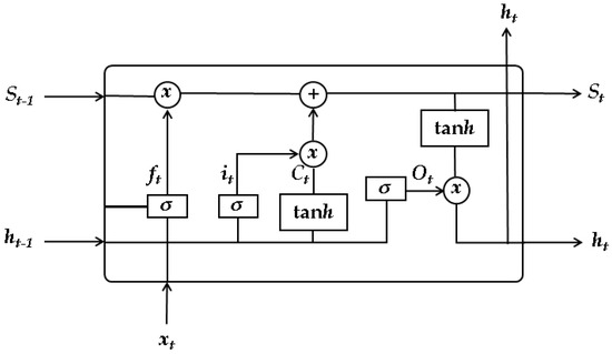
Figure 1.
Schematic of the traditional LSTM network structure.
However, LSTM networks exhibit three distinct limitations in aeroengine RUL prediction:
- (1)
- Computational inefficiency: Sequential processing of high-frequency sensor data leads to prolonged training and inference times.
- (2)
- Poor adaptability to abrupt shifts: LSTM networks struggle to capture sudden degradation (e.g., component faults under extreme conditions) due to their focus on smooth temporal continuity.
- (3)
- Hyperparameter sensitivity: Balancing memory retention and forgetting requires meticulous tuning of gate thresholds and hidden layer dimensions.
3.3. TCN for RUL Prediction
TCNs are 1-dimensional convolutional architectures optimized for sequential data, combining dilated causal convolutions and residual connections [21]. Unlike RNNs, TCNs process sequences in parallel, enabling efficient modeling of long-range dependencies while maintaining computational feasibility.
A key advantage of TCNs lies in the ability to achieve a sufficiently large receptive field via a linear stacking of dilated convolutional layers, enabling the network to model temporal dependencies across extended time spans. To preserve the consistent lengths of the input and output sequences, TCNs adopt a 1-dimensional fully convolutional architecture, ensuring uniform input–output dimensions across all hidden layers by applying zero-padding at the sequence boundaries, a critical feature for maintaining temporal alignment in time series prediction.
To further expand the receptive field and capture multi-scale temporal patterns, TCNs incorporate dilated causal convolutions. These bring exponentially increasing dilation rates (e.g., 1, 2, 4, and 8), which exponentially enlarge the effective historical window without compromising computational efficiency [22]. By exponentially increasing the dilation rate, the network expands its receptive field linearly with each additional layer, eliminating the need for excessively deep architectures when processing long sequences while preserving the integrity of the historical information. This approach allows each layer to capture an exponentially growing effective historical window, striking an optimal balance between modeling long-range temporal dependencies and controlling computational complexity. Formally, the receptive field Rl of the l-th TCN layer can be expressed as follows:
Here, di is the dilation rate of the i-th layer, typically set as di = 2i. Let the input sequence be xt, the convolution kernel be w, and the dilation rate of the l-th layer be dl = 2l. Then, the output yt(l) of the l-th layer with dilation rates dl can be expressed as follows:
where denotes the floor function, ensuring the index t-dl is a non-negative integer.
Additionally, when handling ultra-long sequences, TCNs alleviate vanishing gradients in deep networks, enabling stable training of deeper architectures to model complex degradation dynamics [23]. The output of a causal convolutional layer is calculated through the convolution operation and the activation function:
where w is the convolution kernel, and xt represents the input sequence.
Residual connections integrate the input xt with the convolutional output yt via an element-wise addition operation. Formally, the output zt is expressed as follows:
The residual block design effectively mitigates the vanishing gradient problem inherent in deep networks, enabling stable training even with increasing network depth. When integrated with causal convolutions and dilated convolutions, this unified structure endows TCNs with robust feature extraction capabilities for time series data while preserving computational efficiency. This synergistic combination allows TCNs to simultaneously model short-term fluctuations, medium-term trends, and long-term degradation patterns in aeroengine time series data. By balancing expressive power with computational efficiency, TCNs overcome the key limitations of both CNNs (limited ability to model long-term dependencies) and LSTM networks (sequential computation bottlenecks), making them well-suited for the high-fidelity RUL prediction in dynamic engine operating environments.
3.4. A Hybrid CLSTM-TCN Model Architecture and Design Rationale
3.4.1. Hybrid CLSTM-TCN Model Design
In this section, we propose a hybrid architecture (CLSTM-TCN) integrating three complementary components (2D-CNN, LSTM, and TCN) to enable accurate aeroengine RUL prediction. The module sequence (CNN → LSTM → TCN) is determined by combining their synergistic strengths in capturing distinct features of the input data, following a progressive feature adaptation principle:
- (1)
- 2D-CNN as the Initial Module
CNNs excel at extracting the spatial features via convolutional kernels with local receptive fields. In the proposed CLSTM-TCN model, the 2D-CNN module first processes raw multivariate time series data, extracting local spatial features while effectively capturing short-term temporal patterns and cross-channel interactions through localized convolutions across both temporal and feature dimensions.
- (2)
- LSTM as the Intermediate Module
A two-layer stacked LSTM network (128 hidden units per layer) models long-term temporal dependencies in CNN-processed features, equipped with gated mechanisms (input, forget, and output gates), preserving global degradation trends via its memory cell and gating mechanism. The extracted features are fed into a stacked LSTM network, which leverages its gated architecture to capture the sequential dependencies.
- (3)
- TCN as the Final Module
A three-layer TCN with dilation rates of 1, 2, and 4 captures multi-scale temporal patterns missed by LSTM networks (e.g., sudden degradation spikes). Causal convolutions ensure temporal alignment, while residual connections enhance feature propagation. A fully connected layer projects refined features to RUL predictions.
3.4.2. Rationale for Module Sequencing in CLSTM-TCN Architecture
The CNN→LSTM→TCN sequence is designed to maximize component synergy and minimize information loss, with the position of each module justified by its functional strengths and limitations:
- (1)
- CNN primacy in spatio-temporal processing: Placing the CNN first is critical for filtering spatial noise from raw data, providing clean temporal sequences for subsequent LSTM modeling. Inverting this order (e.g., LSTM→CNN) would force LSTM networks to process unfiltered noise, destabilizing gradient flow.
- (2)
- LSTM network after CNN for sequential modeling: The gated mechanisms (input, forget, and output gates) of LSTM networks are specialized to retain long-term historical information from CNN-processed features, making them ideal for modeling degradation trends. Placing LSTM networks after TCN (e.g., CNN → TCN → LSTM) would truncate critical long-range patterns via TCN’s fixed dilation rates, undermining the strength of LSTM networks in extended dependency modeling.
- (3)
- TCN lasts for multi–scale refinement: The dilated convolutions with exponentially increasing rates of TCN capture multi-scale temporal patterns missed by LSTM networks without increasing model depth. They recover high-frequency short-term details smoothed by LSTM networks, mitigate vanishing gradients via parallel computation, and excel at modeling extended sequences. Early TCN placement (e.g., TCN → CNN → LSTM) prioritizes temporal over spatial patterns, conflicting with data where sensor interactions drive degradation.
This hierarchical sequence (CNN → LSTM → TCN) ensures progressive feature refinement, preventing information bottlenecks and enhancing the capacity of the CLSTM-TCN model to capture complex spatio-temporal dependencies.
The overall architecture (Figure 2) and parameter configurations (Table 1, parameter values are set based on experience and Reference [24]) of the CLSTM-TCN model are designed to balance expressiveness and efficiency, ensuring robust performance on high-dimensional, noisy aeroengine time series.
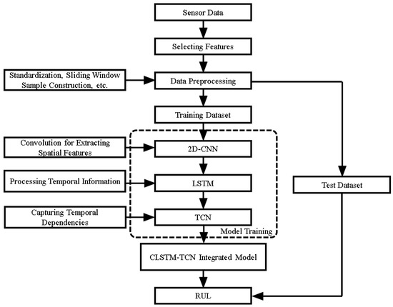
Figure 2.
The overall architecture of CLSTM-TCN.

Table 1.
Module parameter configuration of the proposed CLSTM-TCN model.
3.5. Detailed Modeling Process of CLSTM-TCN
The CLSTM-TCN model follows a systematic workflow spanning data preprocessing, feature extraction, and model training, designed to convert raw sensor data into reliable RUL predictions. The process is structured into six key steps:
- Step 1: Data Preprocessing
- (1)
- Feature Selection: The time series plots of the 24-dimensional raw monitoring features are visualized to identify sensor data with significant degradation trends. Sensors with clear degradation patterns are selected as input features, while irrelevant and redundant information is removed. Through this selection process, the 24-dimensional features were reduced to 14 dimensions, excluding those lacking obvious degradation trends or with high redundancy. The retained effective features serve as inputs for the model, ensuring that the subsequent modeling focuses on the informative signals closely linked to engine degradation.
- (2)
- Data Normalization: To eliminate scale differences in sensor monitoring data, the selected 14-dimensional monitoring feature parameters are normalized. This process converts the raw sensor data into values within the range of [0, 1], standardizing the input space to facilitate stable convergence of the neural network during training and prevent dominant features from overshadowing imperceptible degradation indicators.
- (3)
- Sliding Window for Sample Construction: To fully leverage the temporal information inherent in the sequential data, the sliding window technique is employed to segment the data set into multiple time series samples. A window length W and a step size T are defined, where each sample consists of W consecutive time steps. The step size T governs the overlap between adjacent samples, ensuring the model can effectively learn the evolutionary patterns of the equipment’s operational states.
- (4)
- RUL Labeling: Monitored data are labeled using a piecewise linear function to improve the model’s ability to learn degradation trends. A maximum threshold is defined for the RUL: when the actual RUL exceeds this threshold, it is capped at the maximum value to reduce the excessive variance in labels and enhance the model’s stability, especially in predicting the later stages of engine life characterized by accelerating degradation.
- Step 2: CLSTM Module Processing
As illustrated in Figure 2, the CLSTM module incorporates convolutional layers, ReLU activation functions, pooling layers, and LSTM layers into a unified framework. The preprocessed 14-dimensional feature parameters are fed into the CNN sub-network as the input data. First, the convolutional layers perform temporal convolution on the input data to extract local short-term features, which alleviates the computational burden on the subsequent LSTM layers when processing raw high-dimensional time series data. The ReLU activation function is then applied to introduce non-linearity, enabling the model to capture complex degradation patterns that linear transformations cannot represent and enhancing its overall representational capacity.
A max-pooling layer follows to down-sample the feature maps, reducing computational complexity while retaining the most salient features. The output is subsequently reshaped to match the input dimensions of the LSTM network and forwarded to a two-layer LSTM module, which excels at capturing long-range temporal dependencies and enhancing the modeling of sequential trends inherent in engine degradation processes. To further enhance the model’s robustness, dropout regularization is applied within the LSTM layers for alleviating overfitting to noise or idiosyncrasies in the training data, thereby improving the model’s generalization ability.
- Step 3: TCN Module Refinement
The TCN module adopts a multi-layer dilated convolution structure to capture multi-scale temporal dependencies inherent in aeroengine degradation processes. By utilizing dilated convolutions, it effectively expands the receptive field to cover long-range temporal patterns without increasing computational complexity. Each layer within the TCN module comprises Conv1d, ReLU activation, and Dropout operation, ensuring robust feature extraction while mitigating overfitting. Notably, skip connections are integrated to enhance the feature propagation capability and address the vanishing gradient problem. This module further refines the time series features extracted by the preceding CLSTM module, strengthening the model’s ability to capture both fine-grained temporal fluctuations and coarse-grained degradation trajectories.
- Step 4: Output Layer Prediction
Refined TCN features are passed through a fully connected layer with a linear activation function to project high-dimensional features into a single RUL value, generating the final RUL prediction.
- Step 5: Model Training and Optimization
To enhance the generalization and robustness, the model is trained using an Adam optimizer with weight decay, which mitigates L2 regularization problems compared to the traditional Adam optimizer. Additionally, an early stopping strategy is employed to prevent overfitting by dynamically updating network parameters, ensuring that network parameters balance fitting to training data and the generalization to real engine operating conditions.
- Step 6: Model Evaluation
The prediction accuracy of RUL is quantitatively assessed by combining the root mean square error (RMSE) and the score function (score), ensuring a comprehensive evaluation of the model’s predictive performance.
4. Experiment Results and Analysis
To validate the effectiveness of the proposed CLSTM-TCN framework, we conducted extensive experiments on the NASA C-MAPSS data set, focusing on quantitative performance evaluation and comparative analysis. This section details the experimental setup, data preprocessing, evaluation metrics, and key findings.
4.1. Experimental Data Set and Preprocessing
The C-MAPSS (Commercial Modular Aero-Propulsion System Simulation) data set, developed by NASA, simulates turbofan engine degradation processes and is widely used as a benchmark for RUL prediction [24]. It comprises four sub-data sets (FD001–FD004) with varying operational conditions and fault modes, as summarized in Table 2.
Table 2.
Overview of the C-MAPSS data set.
In this study, the FD001 sub-data set, characterized by a single operational condition and a single fault mode, is selected for analysis, which helps lessen the interference from other conditions and ensures consistency in the framework. The FD001 sub-data set comprises the training set (train_FD001), test set (test_FD001), and RUL labels for the test set (RUL_FD001).
This study focuses on FD001 due to its single operational condition and single fault mode, which minimizes external interference and allows for clear validation of the CLSTM-TCN framework. The data set comprises the training set (train_FD001), the test set (test_FD001), and RUL labels for the test set (RUL_FD001).
The training set includes complete monitoring data of 100 engines, tracking their degradation process from the initial operational state to eventual failure. In contrast, the test set records the operational data of another 100 engines during a specific pre-failure phase, where the exact Remaining Useful Life remains unknown until paired with the RUL_FD001 labels, which provide the actual RUL values for each tested engine.
The tested data set of each engine contains 26 parameters: an engine identifier, cycle count (time step), three operational parameters (Setting 1: flight altitude, Setting 2: Mach number, and Setting 3: throttle lever resolver angle), and 21 sensor-monitored performance parameters, among which, the data format of the 24 monitoring characteristic parameters is detailed in Table 3.
Table 3.
Data format of the 24 monitoring characteristic parameters.
The FD001 data set includes the 24 monitoring characteristic parameters in Table 3, but not all of them effectively reflect the degradation trend. To eliminate the invalid redundant information, a systematic feature screening process was conducted. Through visual analysis of time series trends, eight parameters were identified as invariant across engine operating cycles, including Sensors 1, 5, 6, 10, 16, 18, and 19, and Setting 3. Furthermore, Settings 1 and 2 fluctuated randomly around zero, failing to capture the meaningful degradation information. By excluding these 10 redundant parameters, the other 14 parameters were taken on as valid features and retained as the inputs of the model CLSTM-TCN.
Considering the significant differences among various performance parameters within the value ranges of the engine data set, normalization of the raw monitoring feature parameters is essential to eliminate dimensional disparities between sensor data, improve the training efficiency, and accelerate the convergence rate by ensuring consistent numerical scales across input features.
Here, to standardize the numerical ranges of the raw sensor data while preserving the relative relationships between data points, max–min normalization is utilized to transform them into the interval [0, 1]. The max–min normalization calculation formula is as follows:
where xjmax and xjmin are the maximum and minimum values, respectively, of the j-th monitoring feature parameter data set.
4.2. Evaluation Index
The RMSE is widely used to quantify the discrepancy between the true RUL values and predicted results [20,25,26], providing a measure of the average prediction error magnitude. The calculation formula is as follows:
where N represents the total number of engines, represents the predicted RUL result, and yi represents the true RUL value.
The score function (score) serves as an authoritative evaluation index in aeroengine RUL prediction. As an asymmetric index, it employs different measurement approaches for predicted values: it imposes heavier penalties on delayed predictions and lighter penalties on advanced predictions. Specifically, when the predicted RUL result exceeds the actual remaining life, a more severe penalty is applied. The mathematical expressions are as follows [24]:
4.3. RUL Label Setting
Turbofan engines exhibit a distinct degradation pattern: the performance remains relatively stable in the healthy state before gradually transitioning into a degradation phase. In the initial phase of degradation, the performance decline trend is relatively smooth. However, once the degradation inflection point is crossed, the rate of performance deterioration accelerates significantly.
Aiming at the inherent degradation pattern, we employ a piecewise linear function to label the monitoring data with the piecewise point set at the 125th operating cycle [17] (as illustrated in Figure 3). This segmentation aligns with the observed phase transition in degradation dynamics, ensuring that the RUL labels accurately reflect both the gradual early-stage deterioration and the accelerated late-stage decline. The corresponding rule formula is as follows:
It is obvious that the label value is capped at 125 when the actual RUL of the turbofan engine is greater than or equal to 125 operating cycles. In contrast, when the actual RUL is less than 125 operating cycles, the label decreases sequentially by 1 from 124 down to 1 as the actual RUL drops from 124 to 0. This design ensures that the labels effectively capture the accelerated degradation characteristics after the inflection point while avoiding excessive emphasis on trivial differences in the early stable stage, thus aligning the labeling strategy with the actual degradation trajectory of the engine.

Figure 3.
The piecewise linear function.
Figure 3.
The piecewise linear function.

4.4. Experimental Results
The hybrid CLSTM-TCN model achieves an RMSE of 13.35 and a score of 219 on the test data set, demonstrating strong predictive performance. Figure 4 visualizes the RUL predictions for all 100 engines in the test set, providing a comprehensive overview of the effectiveness of the proposed methodology. As observed in the figure, the predicted RUL values closely align with the actual degradation trajectories for most engines, with only minimal discrepancies across most operational cycles. This widespread consistency confirms the feasibility of the CLSTM-TCN model in capturing aeroengine degradation patterns and validates its effectiveness for RUL prediction.
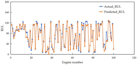
Figure 4.
RUL prediction results for engines on the test data set.
To further quantify the prediction performance of the model, a statistical analysis of the engine RUL prediction errors was conducted, with the results presented in Figure 5 (a histogram of prediction errors). The figure reveals that the distribution of RUL prediction errors approximates a normal distribution (comprehensive statistical tests will be conducted in future research), with most of the errors concentrated within the interval [−20, 20]. This narrow error range, combined with the near-normal distribution, indicates that the prediction biases of the model are randomly distributed rather than exhibiting systematic skewness. Such characteristics further underscore the reliability and stability of the proposed CLSTM-TCN framework for aeroengine RUL prediction.
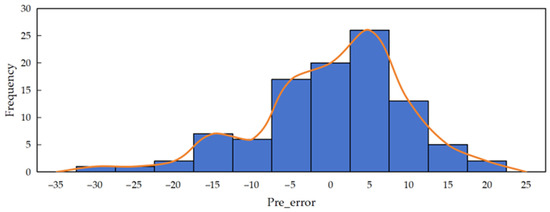
Figure 5.
Histogram of prediction errors.
To validate the predictive performance of the proposed CLSTM-TCN model, four engines (IDs 24, 46, 62, and 76) were randomly selected from the test data set, with their RUL prediction results shown in Figure 6. As clearly illustrated, for all four engines, the predicted RUL curve (blue line) exhibits high consistency with the actual degradation trajectories (orange line) throughout the operational cycles. Notably, in the late stages of the engines’ life (i.e., when RUL approaches 0), the predicted curve shows minimal fluctuations and closely aligns with the actual RUL, effectively capturing the accelerated degradation trend in the final phase. This tight alignment not only confirms the CLSTM-TCN model’s accuracy in modeling late-stage degradation dynamics but also underscores its practical value. By reliably predicting the Remaining Useful Life in the critical late phase, it can provide precise insights for formulating timely and effective maintenance strategies for turbofan engines.
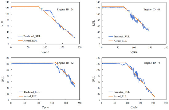
Figure 6.
RUL prediction results for individual engines in the test set (the blue line represents the predicted RUL and the orange line denotes the actual RUL).
5. Ablation Study
To validate the synergistic value of the CLSTM-TCN framework and quantify the contribution of each core module (2D-CNN, LSTM, and TCN), we conducted a systematic ablation study. By sequentially removing one module at a time, we evaluated how each component influences overall predictive performance, ensuring the rationale for their integration.
5.1. Ablation Study Design and Experimental Setup
The primary objective of the ablation study is to assess the effectiveness of each core module (2D-CNN, LSTM, and TCN) within the CLSTM-TCN framework. To rigorously evaluate the role of the 2D-CNN module in extracting local spatial features, it was omitted, resulting in the LSTM-TCN variant. Similarly, the LSTM module was removed to assess its contribution to modeling long-term temporal dependencies, yielding the CNN-TCN model. Finally, the TCN module was excluded to validate its significance in capturing multi-scale temporal feature extraction, resulting in the CNN-LSTM architecture.
To ensure the validity of the experimental results, all ablation experiments were conducted under identical experimental conditions. The NASA C-MAPSS data set was consistently used, with the same training and testing partitions applied across all experiments. Evaluation metrics (RMSE and score) were employed to remain consistent with the primary assessment criteria of the model. A uniform set of hyperparameters, including learning rate, training epochs, batch size, and network layer configurations, was adopted for all ablated models, eliminating confounding variables that might bias performance comparisons.
5.2. Ablation Experiment Results and Analysis
Table 4 summarizes the ablation results from the ablation experiments on the test set. As observed in the table, the CLSTM-TCN model achieves lower RMSE and score values (13.35 and 219, respectively) compared to the model with one of three modules removed: Excluding the TCN (CNN-LSTM) resulted in 38.8% and +131.5% increases in the RMSE and score, respectively, validating its value in capturing multi-scale temporal patterns and mitigating the LSTM network’s vanishing gradient issues. Omitting the LSTM network (CNN-TCN) led to a 44.5% increase in the RMSE and a 169.9% increase in the score, highlighting its importance for modeling long-term degradation trends over hundreds of cycles. Removing the 2D-CNN (LSTM-TCN) increased the RMSE by 44.6% and the score by 163.9%, confirming its critical role in extracting local spatial features and filtering noise from raw sensor data.
Table 4.
Ablation experiment results on the FD001 test set.
To visually illustrate the prediction performance, Figure 7 compares the prediction trajectories of the full model and its ablated variants for a representative engine. It is evident that the CLSTM-TCN curve closely tracks the true RUL degradation trajectories, while ablated models (LSTM-TCN, CNN-TCN, and CNN-LSTM) exhibit larger deviations, particularly in late-stage degradation (remaining life < 100 cycles). This visual alignment reinforces the quantitative results in Table 4, demonstrating that integrating all three modules enables more accurate tracking of non-linear degradation dynamics.
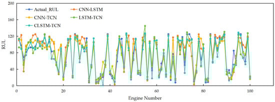
Figure 7.
Comparison chart of prediction results for different models.
To further validate the superiority of the CLSTM-TCN model, the results were compared with published methods [20,25,26] (Table 5), where the best results are highlighted in bold. As shown in Table 5, the CLSTM-TCN model, with an RMSE of 13.35 and a score of 219, demonstrates significant superiority over other comparative models. Specifically, compared with the CNN [20] (RMSE = 18.42, score = 906), the CLSTM-TCN model achieves a 38.0% reduction in the RMSE and a 313.7% reduction in the score; relative to DBN [25] (RMSE = 15.04, score = 334), it reduces the RMSE by 15.6% and the score by 52.5%; versus the CNN-LSTM model [20] (RMSE = 16.36, score = 443), it brings about a 22.5% decrease in the RMSE and a 102.3% decrease in the score; and compared with the LSTM network [26] (RMSE = 16.14, score = 338), it yields a 20.9% reduction in the RMSE and a 54.3% reduction in the score. These results fully confirm the notable advantages of CLSTM-TCN in aeroengine Remaining Useful Life (RUL) prediction.
Table 5.
Performance comparison of RUL predictions with different methods.
6. Conclusions and Discussions
6.1. Conclusions
To address the limitations of single-model architectures in capturing mixed-scale temporal dependencies and enhancing prediction stability, this study proposes a hybrid deep learning framework (CLSTM-TCN) integrating 2D-CNN, LSTM, and TCN modules for aeroengine RUL prediction. Validated on the NASA C-MAPSS data set, the key conclusions are as follows:
- (1)
- The proposed CLSTM-TCN framework achieves complementary advantages through hierarchical design: 2D-CNN effectively extracts short-term local features and inter-feature interactions from the input data, providing a fine-grained feature foundation for subsequent modeling; the LSTM network captures long-term temporal dependencies, preserving global degradation trends across extended cycles; and TCN refines multi-scale temporal patterns via dilated convolutions, overcoming the vanishing gradient issues of the LSTM network and enabling parallel computation for efficiency.
- (2)
- On the FD001 subset of C-MAPSS, the CLSTM-TCN model achieves an RMSE of 13.35 and a score of 219. Ablation studies further confirm that removing any module (2D-CNN, LSTM, or TCN) leads to significant performance degradation: excluding TCN (resulting in CNN-LSTM) increases the RMSE by 38.8% and the score by 131.5%; omitting the LSTM network (resulting in CNN-TCN) raises the RMSE by 44.5% and the score by 169.9%; and removing 2D-CNN (resulting in LSTM-TCN) causes the RMSE to increase by 44.6% and the score by 163.9%. Compared to hybrid baselines (CNN-LSTM, CNN-TCN, and LSTM-TCN), it reduces the RMSE by 27.94–30.88% and maintains stability across test cases (RMSE fluctuations < 15%), verifying its reliability in a complex operational environment.
- (3)
- CLSTM-TCN outperforms published methods (CNN [20], DBN [25], CNN-LSTM [20], and LSTM [26]) in the RMSE by 15.6–38.0% (38.0% vs. CNN [20], 15.6% vs. DBN [25], 22.5% vs. CNN-LSTM [20], and 20.9% vs. the LSTM network [26]) and in the score by 52.5–313.7%, demonstrating its superiority in modeling the non-linear, multi-phase degradation dynamics of aeroengines.
6.2. Discussions
Despite the promising performance of the CLSTM-TCN model in aeroengine RUL prediction, methodological limitations and practical challenges remain, guiding future research to enhance its robustness and practicality.
6.2.1. Current Limitations
- (1)
- Data Dependency: The performance of the CLSTM-TCN model is primarily reliant on high-quality, large-scale data sets. In data-scarce scenarios (e.g., newly deployed engines or rare operating conditions), insufficient training samples lead to degraded prediction accuracy, limiting adaptability to novel environments.
- (2)
- Computational Complexity: Integrating 2D-CNN, LSTM, and TCN incurs high computational costs, leading to prolonged training and inference times. This hinders real-time deployment in time-sensitive aviation applications where rapid RUL updates are critical for maintenance decisions.
- (3)
- Hyperparameter Sensitivity: The model exhibits high sensitivity to key hyperparameters, including learning rate, convolution kernel size, LSTM hidden layer dimensions, and TCN dilation rates. Extensive manual tuning is required to achieve optimality, increasing the implementation complexity.
6.2.2. Future Research Directions
To address these limitations, future work will focus on the following areas.
- (1)
- Enhancing Adaptability to Complex Operating Conditions: The current study is constrained to RUL prediction of turbofan engines under static, single operating conditions, with insufficient consideration of real-world complexities, specifically, multi-condition operations and dynamic shifts in operational parameters, which are prevalent in practical aviation scenarios. This narrow scope limits the model’s adaptability and generalizability across the diverse operational landscapes encountered in engineering practice. To address this issue, future research will expand the scope to systematically explore life-cycle modeling under multi-condition and variable-condition regimes. Key efforts will include developing tailored transfer learning frameworks and domain adaptation methodologies to enable robust generalization across heterogeneous operational scenarios, thereby enhancing the model’s practical utility in real-world aviation environments.
- (2)
- Integrating Uncertainty Analysis Mechanisms: In aviation, quantifying the uncertainty in model predictions is foundational to robust risk control and data-driven decision making. However, current research in this domain remains predominantly reliant on RMSE- and score-based metrics for statistical evaluation, which fail to comprehensively characterize uncertainty distributions or rigorously assess prediction credibility. To bridge this critical gap, future work will integrate Bayesian deep learning frameworks, confidence interval estimation, and Monte Carlo dropout sampling methods to explicitly quantify aleatoric and epistemic uncertainties. This enhancement will not only enhance the interpretability and reliability of the predictive outputs but also deliver actionable insights that strengthen risk mitigation protocols and decision support systems in safety-critical aviation operations.
- (3)
- Advancing Multi-Model Fusion Strategies: The current framework adopts a static serial integration paradigm to combine model components, while this validates the value of modular collaboration, it lacks flexibility in adapting to dynamic data patterns. Future research will transcend this fixed structure by exploring adaptive fusion mechanisms, including dynamic weighting schemes, attention-driven feature aggregation, and multi-task learning architectures. These advanced strategies will be designed to more effectively leverage the intrinsic complementarity between heterogeneous models (e.g., CNNs for spatial patterns, LSTM networks for temporal sequences, and TCNs for multi-scale dependencies) and amplify their synergistic effects. By enabling context-aware integration of model outputs, such approaches have the potential to enhance prediction accuracy while preserving computational efficiency, thereby strengthening the model’s performance in complex aviation scenarios.
- (4)
- Exploring Module Order Variations: The current module order (CNN→LSTM→TCN) aligns with the hierarchical spatio-temporal characteristics of the data set. Future work will conduct a rigorous ablation study to systematically evaluate alternative configurations. This comprehensive investigation will encompass the following three key dimensions:
- Quantifying performance trade-offs across all permutations of the modules, such as LSTM→CNN→TCN and TCN→LSTM→CNN, with a focus on metrics such as prediction accuracy, convergence stability, and error distribution patterns.
- Analyzing computational efficiency and scalability across different architectural orders to identify configurations optimized for real-world deployment.
- Investigating task-specific sensitivities by validating these module permutations on diverse data sets characterized by varying spatio-temporal dynamics, ranging from high-frequency industrial sensors to long-term sequential data, thereby assessing generalizability beyond aviation-specific scenarios.
- (5)
- Mitigating Data Dependency and Computational Burden: To address the model’s reliance on large-scale data sets and high computational overhead, future work will focus on developing lightweight network architectures, incorporating techniques such as parameter pruning, knowledge distillation, and efficient convolution operators, to reduce computational costs without sacrificing predictive performance. Concurrently, few-shot and zero-shot learning frameworks will be integrated to enhance adaptability to data-scarce scenarios.
- (6)
- Optimizing Hyperparameter Tuning: To alleviate the complexity of implementation, future work will focus on designing adaptive hyperparameter optimization frameworks and automated tuning pipelines. These systems will dynamically adjust critical parameters, such as learning rates, convolution kernel sizes, and LSTM hidden layer dimensions, based on data set characteristics and task requirements. By streamlining the tuning process, this advancement will ensure consistent model performance across diverse data sets while enhancing accessibility for practical deployment, reducing the technical barrier for engineers and researchers in aviation applications.
Author Contributions
Conceptualization, B.T. and L.W.; validation, Y.C. and Y.F.; data curation, Y.Z. and Y.C.; writing—original draft preparation, B.T., X.W. and Y.Z.; writing—review and editing, L.W., Y.F., L.Z. and C.G.R.L.R.; project administration, B.T.; funding acquisition, B.T. All authors have read and agreed to the published version of the manuscript.
Funding
This research was funded by the National Natural Science Foundation of China (41876219), the Key Science Foundation for Universities of Henan Province (24A110008), the Senior-end Foreign Expert Introduction Project of Henan Province (HNGD2025034), and the Cultivation Project of the National Natural Science Foundation of China, Youth Science Foundation Project of Nanyang Normal University (2025QN016).
Data Availability Statement
The data used to support the findings of this study are all included in the article. For a more detailed data request, please contact the corresponding authors directly.
Acknowledgments
The authors gratefully acknowledge Zhijun Li and Qiuming Zhao at Dalian University of Technology for their assistance in editing the structure of this manuscript.
Conflicts of Interest
The authors declare no conflicts of interest. The funders had no role in the design of the study; in the collection, analyses, or interpretation of data; in the writing of the manuscript; or in the decision to publish the results.
References
- Khelif, R.; Chebel–Morello, B.; Malinowski, S.; Laajili, E.; Fnaiech, F.; Zerhouni, N. Direct remaining useful life estimation based on support vector regression. IEEE Trans. Ind. Electron. 2017, 64, 2276–2285. [Google Scholar] [CrossRef]
- Zio, E. Prognostics and Health Management (PHM): Where are we and where do we (need to) go in theory and practice. Reliab. Eng. Syst. Saf. 2022, 218, 108119. [Google Scholar] [CrossRef]
- Cai, Z.Y.; Wang, Z.Z.; Chen, Y.X.; GUO, J.S.; Xiang, H.C. Remaining useful lifetime prediction for equipment based on nonlinear implicit degradation modeling. J. Syst. Eng. Electron. 2020, 31, 198–209. [Google Scholar] [CrossRef]
- Zhang, X.; Tang, S.; Liu, T.; Zhang, B. A new residual life prediction method for complex systems based on wiener process and evidential reasoning. J. Control Sci. Eng. 2018, 2018, 9473526. [Google Scholar] [CrossRef]
- Wang, C.; Yang, B.; Zhu, T.; Xiao, S.N.; Yang, G.; Fan, X. Research on crack propagation and residual life prediction method of surface–strengthened axle. J. Mech. Eng. 2023, 59, 43–53. [Google Scholar]
- Zhang, X.; Liu, Y. Research on residual life prediction of aeroengine based on knowledge distillation compression mixing model. Comput. Integr. Manuf. Syst. 2025, 31, 290–305. [Google Scholar]
- Zhang, H.; Long, L.; Dong, K. Detect and evaluate dependencies between aeroengine gas path system variables based on multi scale horizontal visibility graph analysis. Phys. A Stat. Mech. Its Appl. 2019, 526, 120830. [Google Scholar] [CrossRef]
- Peng, H.B.; Liu, M.M.; Wang, Y.G. Research on life prediction of aeroengine based on take–off exhaust temperature margin (EGTM). Sci. Technol. Eng. 2014, 14, 160–164. [Google Scholar]
- Gu, M.Y.; Ge, J.Q.; Li, Z.N. Improved similarity–based residual life prediction method based on grey markov model. J. Braz. Soc. Mech. Sci. Eng. 2023, 45, 294–306. [Google Scholar] [CrossRef]
- Song, Y.; Xia, T.; Zheng, Y.; Zhuo, P.; Pan, E. Prediction of remaining life of turbofan engine based on auto encoder–BLSTM. Comput. Integr. Manuf. Syst. 2019, 25, 1611–1619. [Google Scholar]
- Ren, L.; Cui, J.; Sun, Y.; Cheng, X. Multi–bearing remaining useful life collaborative prediction: A deep learning approach. J. Manuf. Syst. 2017, 43, 248–256. [Google Scholar] [CrossRef]
- Babu, G.S.; Zhao, P.; Li, X.L. Deep convolutional neural network based regression approach for estimation of remaining useful life. In Proceedings of the International Conference on Database Systems for Advanced Applications, Dallas, TX, USA, 16–19 April 2016; pp. 214–228. [Google Scholar]
- Zhang, X.; Qin, Z.; Li, M.; Shi, J. Prediction of remaining life of aeroengine based on multi–feature fusion. J. Comput. Syst. Appl. 2023, 32, 95–103. [Google Scholar]
- Yu, P.; Wang, H.; Cao, J. Aero–engine residual life prediction based on time–series residual neural networks. J. Intell. Fuzzy Syst. Appl. Eng. Technol. 2023, 45, 2437–2448. [Google Scholar] [CrossRef]
- He, Y.; Wen, C.; Xu, W. Residual life prediction of SA-CNN-BILSTM aero-engine based on a multichannel hybrid network. Appl. Sci. 2025, 15, 966. [Google Scholar] [CrossRef]
- Huang, M.; Yang, L.; Jiang, G.; Hao, X.; Lu, H.; Luo, H.; Wang, P.; Li, J. Rescconv–xlstm: An improved xlstm model with spatiotemporal feature extraction capability for remaining useful life prediction of aero–engine. Results Eng. 2025, 26, 105513. [Google Scholar] [CrossRef]
- Al–Dulaimi, A.; Zabihi, S.; Asif, A.; Mohammadi, A. A multimodal and hybrid deep neural network model for remaining useful life estimation. Comput. Ind. 2019, 108, 186–196. [Google Scholar] [CrossRef]
- Lyu, D.; Hu, Y. Remaining useful life prediction of aeroengine based on principal component analysis and one-dimensional convolutional neural network. Trans. Nanjing Univ. Aeronaut. Astronaut. 2022, 38, 867–875. (In Chinese) [Google Scholar] [CrossRef]
- Liu, Q.; Dai, Z.; Chen, P.; Lai, H.; Liang, Y.; Chen, M.; Xu, X.; Hou, M.; Wang, G. Remaining useful life prediction of rolling bearings based on TCN–LSTM. In Proceedings of the 14th International Conference on Quality, Reliability, Risk, Maintenance, and Safety Engineering (QR2MSE 2024), Harbin, China, 24–27 July 2024; pp. 1016–1020. [Google Scholar]
- Li, J.; Jia, Y.J.; Zhang, Z.X.; Li, R.R. Prediction of remaining life of aeroengine based on fusion neural network. Propuls. Technol. 2021, 42, 1725–1734. [Google Scholar]
- Ji, W.; Cheng, J.; Chen, Y. Remaining useful life prediction for mechanical equipment based on temporal convolutional network. In Proceedings of the 14th IEEE International Conference on Electronic Measurement and Instruments (ICEMI), Changsha, China, 1–3 November 2019; pp. 1192–1199. [Google Scholar]
- Yang, W.; Yao, Q.; Ye, K.; Xu, C.Z. Empirical mode decomposition and temporal convolutional networks for remaining useful life estimation. Int. J. Parallel Program. 2020, 48, 61–79. [Google Scholar] [CrossRef]
- He, K.; Zhang, X.; Ren, S.; Sun, J. Deep residual learning for image recognition. In Proceedings of the IEEE Conference on Computer Vision and Pattern Recognition 2016, Las Vegas, NV, USA, 27–30 June 2016; pp. 770–778. [Google Scholar]
- Saxena, A.; Goebel, K.; Simon, D.; Eklund, N. Damage propagation modeling for aircraft engine run-to-failure simulation. In Proceedings of the 2008 International Conference on Prognostics and Health Management, Denver, CO, USA, 6–9 October 2008; pp. 1–9. Available online: https://ieeexplore.ieee.org/document/4711414/ (accessed on 16 June 2025).
- Zhang, C.; Lim, P.; Qin, A.K.; Tan, K.C. Multiobjective deep belief networks ensemble for remaining useful life estimation in prognostics. IEEE Trans. Neural Netw. Learn. Syst. 2016, 28, 2306–2318. [Google Scholar] [CrossRef] [PubMed]
- Zheng, S.; Ristovski, K.; Farahat, A.; Gupta, C. Long short–term memory network for remaining useful life estimation. In Proceedings of the 2017 IEEE International Conference on Prognostics and Health Management, Dallas, TX, USA, 19–21 June 2017; pp. 88–95. [Google Scholar]


Disclaimer/Publisher’s Note: The statements, opinions and data contained in all publications are solely those of the individual author(s) and contributor(s) and not of MDPI and/or the editor(s). MDPI and/or the editor(s) disclaim responsibility for any injury to people or property resulting from any ideas, methods, instructions or products referred to in the content. |
© 2025 by the authors. Licensee MDPI, Basel, Switzerland. This article is an open access article distributed under the terms and conditions of the Creative Commons Attribution (CC BY) license (https://creativecommons.org/licenses/by/4.0/).