Abstract
In this work, we proposed a dynamic inverse solution with spatio-temporal constraints of the nonlinear heat diffusion problem in 1D and 2D based on a regularized Gauss–Newton and Krylov subspace with a preconditioner. The preconditioner is computed by approximating the Jacobian of the nonlinear system at each Gauss–Newton iteration. The proposed approach is used for estimation of the initial value from measurements of the last value by considering spatial and spatio-temporal constraints. The system is compared to a dynamic Tikhonov inverse solution and generalized minimal residual method (GMRES) with and without a preconditioner. The system is evaluated under noise conditions in order to verify the robustness of the proposed approach. It can be seen that the proposed spatio-temporal regularized Gauss–Newton method with GMRES and a preconditioner shows better estimation results than the other methods for both spatial and spatio-temporal constraints.
1. Introduction
Nonlinear inverse problems arise frequently in engineering and applied sciences, particularly in systems governed by nonlinear partial differential equations. These problems are often ill-posed, meaning that small perturbations in the data can lead to large deviations in the solution, making regularization techniques essential for obtaining stable and meaningful results. In [1], several methods are considered for the solution of the linear and nonlinear inverse problems in practical applications, such as image deblurring, X-ray tomography, backward parabolic problems, heat transfer or diffusion, and electrical impedance tomography. In [2], the integration of model-based and data-driven techniques to enhance stability and generalizability in inverse reconstructions is presented. For example, in [3], a Jacobian-Free Newton–Krylov (JFNK) method is introduced to address tumour growth modeling, a highly nonlinear and ill-posed setting. The authors develop efficient preconditioning strategies that improve the convergence of the Krylov inverse solver without the need to compute or store Jacobians explicitly, making the approach particularly suitable for large-scale biomedical simulations and also generalizable to other applications.
Other adaptive and scalable strategies have also been introduced to improve the performance and robustness of nonlinear inverse problem solvers. A classical and widely studied approach is the iteratively regularized Gauss–Newton method, introduced by [4], which incorporates regularization at each iteration to stabilize the solution process. This method has proven effective for nonlinear ill-posed problems and is supported by rigorous convergence theory. More recently, in [5] an efficient implementation of the Gauss–Newton method using generalized Krylov subspaces is developed, significantly improving computational performance for large-scale problems. Their approach also integrates Broyden-type secant updates to approximate the Jacobian, reducing the computational cost in nonlinear settings. In parallel, Rajan and Jose [6] addressed the discretization challenges associated with nonlinear inverse problems, proposing a scheme that enhances stability and convergence by maintaining the structural fidelity of the continuous problem. These advances highlight the ongoing need for methods that are not only accurate and robust but also scalable and adaptable to complex, time-dependent systems. In [7], a learning-based regularization framework is proposed using deep neural networks to model complex solution manifolds in inverse problems, enabling data-driven priors in ill-posed nonlinear settings. Moreover, Zhao et al. [8] introduces a regularized Newton–GMRES method that combines regularization with iterative solvers, enhancing convergence and stability for nonlinear systems. Despite these advances, most methods still assume static or homogeneous priors and do not explicitly model spatio-temporal dependencies in the solution space.
The dynamic inverse problem of recovering the initial condition in nonlinear heat diffusion systems presents significant challenges due to its ill-posedness, nonlinearity, and sensitivity to noise. In [9,10,11], the inverse heat conduction problem and the traditional computational methods used for its solution are presented with applications in the areas of manufacturing, aerospace, biomedical, and electronics cooling. In these reviews, two main factors are considered for almost all the applications: a detailed knowledge of the heat equation (forward problem) and the use of a regularized cost function for the solution of the ill-posed ill-conditioned problem. However, traditional approaches often treat spatial and temporal regularization independently or rely on static formulations that fail to take advantage of the underlying dynamics of the system by considering only the solution of an optimization problem [12].
In [13], the authors proposed the numerical solution by Tikhonov regularization of the surface heat flux history and temperature distribution in an inverse heat conduction problem with a nonlinear source term. Similarly, Shidfar et al. [14] presents an inverse heat conduction problem with a nonlinear source term, where the surface heat flux history of a heated conducting body is identified by approximating the unknown function using linear polynomial pieces determined from an optimization problem. Moreover, Liu et al. [15] propose a multigrid-based framework integrated with constraint data assimilation to solve inverse problems governed by nonlinear diffusion equations. Their method improves both accuracy and computational speed by exploiting multi-resolution grid structures and incorporating measurement constraints at different scales. For instance, in [16], the authors propose a solution to the inverse heat conduction problem in a one-dimensional domain with a moving boundary and temperature-dependent material properties, emphasizing the need for robust methods capable of handling dynamic, nonlinear systems. In addition, in [17], a fast, robust, and automatic selection of the regularization parameter in inverse heat conduction problems is proposed for linear and nonlinear systems, which facilitates the tuning of the inverse problem solution. Also, Ciofalo [18] explores the solution of an inverse heat conduction problem to reconstruct the steady-state distribution of the convection heat transfer coefficient on one wall of a slab from the temperature distribution on a plane embedded in the slab, assuming that the thermal boundary conditions on the other walls are known. However, while these methods emphasize solver efficiency or domain adaptation, they do not address the integration of spatio-temporal constraints directly into the regularization process.
In this work, we propose a spatio-temporal regularized Gauss–Newton method combined with GMRES and an efficient preconditioning strategy to solve the nonlinear heat equation in both 1D and 2D domains. The preconditioner is constructed by approximating the Jacobian of the nonlinear system at each Gauss–Newton iteration, enhancing convergence and numerical stability. The proposed approach is evaluated in the context of an initial value reconstruction problem, where the goal is to estimate the initial state from final-time measurements, incorporating both spatial and spatio-temporal regularization constraints. By embedding these constraints into a dynamic regularization framework, our method aims to bridge the gap between physical realism, computational feasibility, and generalizability across diverse nonlinear inverse problems. We compare our method against state-of-the-art alternatives, including a dynamic Tikhonov inverse solution and the GMRES method with and without preconditioning.
The main contributions of this work are as follows:
- •
- Spatio-Temporal Regularized Inverse Framework: We propose a dynamic inverse solution that incorporates spatio-temporal regularization constraints directly into the cost functional. This allows the reconstruction to respect both spatial smoothness and temporal consistency.
- •
- Integration with Krylov Subspace Solvers: The nonlinear inverse problem is solved using a regularized Gauss–Newton method, where each linearized step is efficiently computed using the GMRES algorithm. This Krylov-based approach enables scalability to large problem sizes.
- •
- Jacobian-Based Preconditioning: A lightweight preconditioner is introduced by approximating the Jacobian at each iteration, significantly enhancing convergence and numerical stability of the GMRES solver in both 1D and 2D.
The remainder of this paper is organized as follows: Section 2 introduces the nonlinear diffusion problem. Section 3 details the proposed Spatio-Temporal Regularized Gauss–Newton method, including its integration with GMRES and the preconditioner design. Section 4 and Section 5 present the numerical results, performance evaluation, and concluding remarks based on the comparative analysis with existing estimation techniques.
2. Nonlinear Diffusion Problem
2.1. Nonlinear 1D Diffusion
We consider the general nonlinear diffusion equation, also known as the porous medium equation, as described in [19], as follows:
where
is the diffusion coefficient defined by
where m is the order of the nonlinearity. The system is subject to homogeneous Neumann boundary conditions:
which physically represent no-flux conditions at the boundaries. We complete the initial boundary value problem by specifying the initial condition:
where
is a sufficiently regular function. The well-posedness of the nonlinear diffusion Equation (1) with Neumann boundary conditions and a smooth, strictly positive initial condition has been studied in [19], guaranteeing existence, uniqueness, and continuous dependence of the solution on the data for
.
The approximation of (1) can be formulated by using the explicit finite difference discretization of the nonlinear diffusion equation. Let
denote the numerical approximation of
and
the diffusion coefficient evaluated at
. The explicit scheme is given by:
for
.
The Neumann boundary conditions are discretized as:
which means that there is no flow of the diffusing quantity across the boundaries.
The explicit scheme can be summarized as
where
is the nonlinear discretization of the nonlinear diffusion equation l steps ahead.
The explicit scheme is first-order accurate in time and second-order accurate in space, assuming sufficient smoothness of the solution
[20]. That is, the local truncation error satisfies:
Stability of the explicit scheme is governed by a nonlinear generalization of the Courant–Friedrichs–Lewy (CFL) condition [21]:
to prevent instabilities and ensure boundedness of the numerical solution. This condition becomes more restrictive for large values of m or sharply peaked initial profiles. The convergence of the scheme follows from consistency and stability (under the CFL condition), and can be justified using a nonlinear generalization of Lax’s equivalence theorem [22], provided the solution remains smooth and the step sizes are properly chosen.
2.2. Nonlinear Diffusion Problem in 2D
We now consider the extension of the nonlinear diffusion equation (also known as the porous medium equation) to two spatial dimensions, as described in [19]:
where
is the nonlinear diffusion coefficient, and
is the nonlinearity parameter. We consider Neumann boundary conditions on the boundary
:
where
denotes the outward normal to the boundary, indicating that there is no flux across the domain boundaries. We complete the initial boundary value problem by prescribing the initial condition:
where
is a regular function, and
. For
, this condition ensures the well-posedness of (6), including existence, uniqueness, and continuous dependence on the initial data, as discussed in [19].
To numerically approximate (6), we consider a uniform grid over a rectangular domain
, with grid spacings
and
, and time step
. Let
denote the approximation to
, and
. The explicit finite difference scheme can be written as:
for
,
. The Neumann boundary conditions are enforced using ghost points or mirrored values. A simple first-order approximation gives:
This reflects the assumption of zero gradient (i.e., no flux) at the boundary. The explicit scheme can also be summarized by a nonlinear operator
, which propagates the solution l steps forward in time:
where
depends nonlinearly on the values of u through the coefficient
.
The explicit scheme is first-order accurate in time and second-order accurate in space, assuming that
is smooth enough [20]. That is, the local truncation error is given by:
For stability, the time step must satisfy a two-dimensional generalization of the CFL condition [21]:
This condition ensures numerical stability and must be respected, especially when
or when u develops sharp gradients. The convergence of the scheme, under this condition, can be justified for smooth solutions via nonlinear extensions of Lax’s equivalence theorem [22].
This formulation serves as the basis for the forward simulation in inverse problems or data assimilation frameworks involving nonlinear parabolic PDEs in two dimensions. In the context of the inverse problem, this formulation is often vectorized by reshaping the matrix-valued solution
into a column vector
. This allows the forward operator
to be implemented as a nonlinear mapping in vector space, facilitating the application of optimization-based reconstruction methods.
3. Dynamic Inverse Solution by Gauss–Newton
The inverse problem is as follows: given a noisy observation
at final time T, recover the initial condition
. This inverse problem is analyzed in [23,24] by considering a linear diffusion coefficient. It is worth noting that if T is too large, the solution of the heat equation tends to a spatially homogeneous (stationary) state due to the strong smoothing effect of diffusion. As a result, the inverse problem becomes severely ill-posed, since high-frequency components of the initial condition are exponentially damped and become unrecoverable from the final data.
This ill-posedness manifests in the decay of the singular values of the forward operator, which becomes more pronounced as T increases. For instance, in the linear 1D heat equation with homogeneous Neumann or Dirichlet boundary conditions, the Fourier or eigenmode components decay like
, where
are the eigenvalues of the Laplacian. This implies that larger values of T result in more significant loss of information, especially in higher modes. Therefore, there exists a practical upper limit for the observation time T, beyond which the data
no longer contain sufficient information to accurately reconstruct the initial condition. The precise restriction depends on the spatial resolution, the noise level, and the regularity of the initial condition. In practice, moderately small values of T are preferred to balance physical diffusion and numerical stability.
To address the instability for large T, it is necessary to incorporate regularization algorithms (e.g., Tikhonov, TV, or iterative regularization methods) that stabilize the inversion and suppress amplification of noise during reconstruction. The Gauss–Newton method is a widely used iterative approach for solving nonlinear inverse problems, particularly when the forward model can be linearized in the neighborhood of the current estimate. A rigorous formulation and convergence analysis of this method is provided in [5], where the authors propose an efficient implementation based on projections into generalized Krylov subspaces. Their framework allows the Gauss–Newton method to be applied effectively to large-scale problems by iteratively building a sequence of low-dimensional subspaces that approximate the solution space. Importantly, the convergence of the proposed algorithm is theoretically established under standard assumptions, and its numerical performance is demonstrated across several examples. This formulation provides a solid theoretical and computational foundation upon which we build in this work, extending the approach with spatio-temporal regularization and preconditioning strategies to address dynamic inverse problems governed by nonlinear diffusion equations. In this case, we proposed a regularized dynamic inverse solution with spatio-temporal constraints based on the Gauss–Newton method with preconditioned Krylov subspaces (by means of the GMRES algorithm). The proposed approach is described in Section 3.1 and Section 3.2.
3.1. Regularized Inverse Solution with Spatio-Temporal Constraints
A generalized cost function with spatio-temporal constraints can be defined as
where
- •
- denotes the forward nonlinear model evaluated at final time T at sample (), with initial condition ;
- •
- is the regularization parameter;
- •
- L is the spatial constraint;
- •
- is the temporal regularization parameter;
- •
- represents the approximate solution at time , with .
3.2. Gauss–Newton Iterative Scheme for the Spatio-Temporal Regularized System with GMRES
The Gauss–Newton method iteratively linearizes the forward model and solves a regularized linear system [25]. At iteration k, we perform the following steps:
- Simulate the forward model at the current guess of the initial condition at iteration:
- Compute the residual:
- Compute the Jacobian matrix of the forward model with respect to the initial condition:
- Define the left-hand-side operator for the linearized system:with computed as:
- Define the right-hand side:with computed as
- Solve the regularized linear system:using the GMRES algorithm, where a preconditioner is used to accelerate convergence, resulting en the system
- Update the estimate of the initial condition:
- Check convergence:
This process is repeated until convergence is achieved. Unlike a single-step linearized Tikhonov method or GMRES method, Gauss–Newton refines both the solution and the local linearization at each iteration, making it more robust for strongly nonlinear models such as the case where
.
3.3. Regularized Inverse Solution with Spatial Constraints
Since we are considering a nonlinear dynamic system, the following regularized nonlinear problem with spatial constraints can be defined:
which is the cost function for spatio-temporal constraints but considering the temporal regularization parameter
.
3.4. Gauss–Newton Iterative Scheme for the Spatially Regularized System with GMRES
The Gauss–Newton method considered in the last section is applied iteratively, replacing only the steps 4 and 5 as follows:
- 4.
- Define the left-hand-side operator for the linearized system:
- 5.
- Define the right-hand side:
This process is repeated until convergence is achieved.
3.5. Jacobian Approximation
We approximate the Jacobian of the nonlinear mapping
at the k-th Gauss–Newton iteration, by using central differences [26], as follows:
where
is a small perturbation step size, and
is the unit vector in the i-th direction. This gives a second-order accurate approximation to the true Jacobian at iteration k.
3.6. Preconditioner Selection
The preconditioner
is computed at each iteration by considering
Therefore,
is equivalent to solving a system that is closer to identity, and thus the solver converges much faster.
4. Results
In order to evaluate the proposed approach for the dynamic inverse solution by the proposed Gauss–Newton with GMRES and a preconditioner, a forward problem with a nonlinear system diffusion equation for the 1D and 2D cases is analyzed, and the estimation results are compared with the Gauss–Newton method using Tikhonov and GMRES without a preconditioner.
4.1. One-Dimensional Estimation Results
Initially, the forward problem with a nonlinear system diffusion equation for the 1D case is considered with
and with initial condition
defined by
with
,
,
,
. To ensure the stability of the explicit numerical scheme, the time step
must satisfy the nonlinear CFL condition given by (5). Since the maximum of the initial condition is
, and replacing the values in (5), the following calculation is obtained:
Since the selected time step is
, the CFL condition is satisfied.
The space-time dynamic behavior of the nonlinear diffusion equation without noise is shown Figure 1.
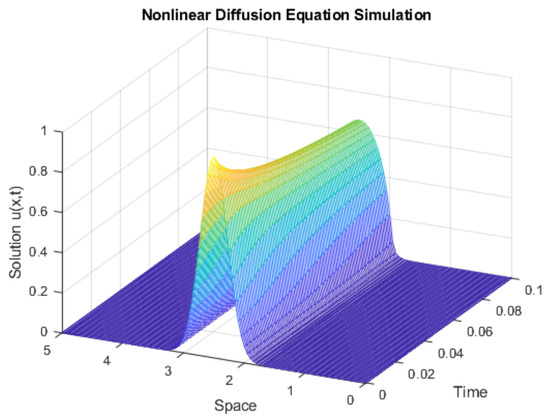
Figure 1.
Space-time dynamic behavior of the nonlinear diffusion equation.
The observed
with an additive noise of
is shown in Figure 2.
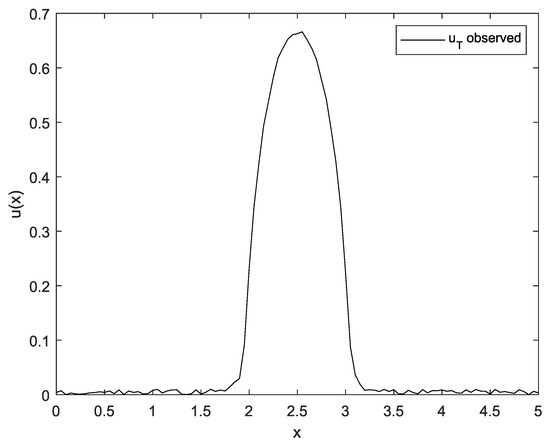
Figure 2.
Observed
.
The performance of the proposed approach is evaluated and compared with spatial and spatio-temporal constraints and considering several methods for the solution of the resulting regularized system in the Gauss–Newton method. The tolerance value
to check the convergence of the Gauss–Newton algorithm is
. In addition, the algorithm is restricted to a maximum of 20 iterations.
4.1.1. Dynamic Inverse Solution with Spatial Constraints
The
estimated solution is computed by using the proposed approach computing the spatially regularized Gauss–Newton system solution by the GMRES algorithm with and without a preconditioner and the exact Tikhonov solution assuming
, where the selection of
is performed by considering the trade-off between the norm of a regularized solution and its fit to the given data (L-curve method) [24].
The estimated
from observed
by using the Tikhonov regularized solution, with
, is shown in Figure 3.
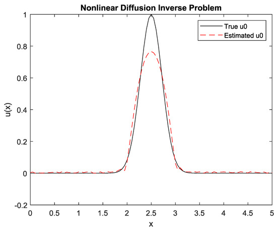
Figure 3.
Estimated
by Tikhonov spatial regularization.
The estimated
from observed
by using the GMRES without the preconditioner for the regularized solution with
is shown in Figure 4.
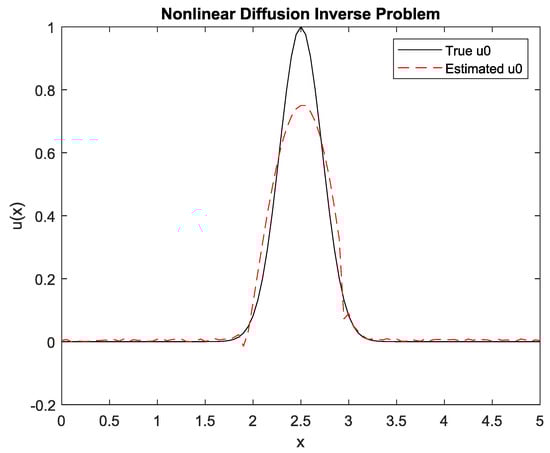
Figure 4.
Estimated
by GMRES regularization without a preconditioner.
The estimated
from observed
by using the GMRES with a preconditioner of the regularized solution with
is shown in Figure 5.
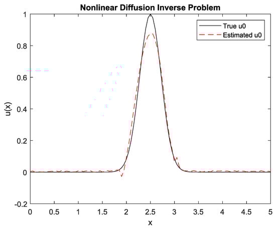
Figure 5.
Estimated
by GMRES regularization with a preconditioner.
4.1.2. Dynamic Inverse Solution with Spatio-Temporal Constraints
The
estimated solution is computed by using the proposed approach computing the spatio-temporal regularized Gauss–Newton system solution by the GMRES algorithm with and without a preconditioner and the exact Tikhonov, where the selection of
and
are performed by considering the trade-off between the norm of the regularized spatial solution, the temporal solution, and its fit to the given data (L-surface method or L-curve generalization for multiple constraints).
The estimated
from the observed
by using the Tikhonov spatio-temporal regularized solution, with
and
, is shown in Figure 6.

Figure 6.
Estimated
by Tikhonov spatio-temporal regularization.
The estimated
from the observed
by using the GMRES without the preconditioner for the regularized spatio-temporal solution with
and
is shown in Figure 7.
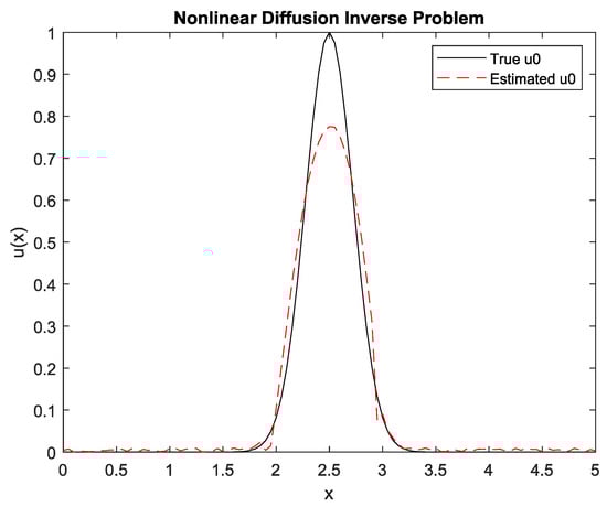
Figure 7.
Estimated
by GMRES spatio-temporal regularization without a preconditioner.
The estimated
from observed
by using the GMRES with a preconditioner of the regularized spatio-temporal solution with
and
is shown in Figure 8.
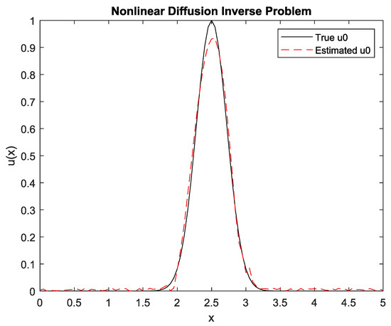
Figure 8.
Estimated
by GMRES spatio-temporal regularization with a preconditioner.
It can be seen from Figure 6, Figure 7 and Figure 8, that the GMRES spatio-temporal regularization with a preconditioner is the solution that best approximates the true
even if the spatio-temporal regularization is compared with the spatial regularization.
Figure 9 shows a comparison of the 3D simulation (noiseless) of the nonlinear diffusion equation shown in Figure 1, and the resulting constrained estimation surface for all the time interval
by considering the proposed GMRES spatio-temporal regularization with a preconditioner is shown.
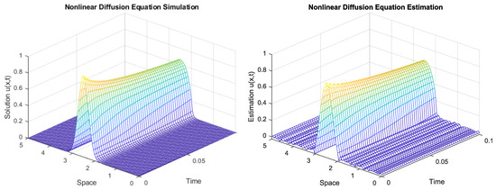
Figure 9.
Space-time dynamic simulation and constrained estimation surface of the nonlinear diffusion equation by considering the proposed GMRES spatio-temporal regularization with a preconditioner.
It is worth noting from Figure 9 that the constrained estimation surface of the nonlinear diffusion equation is similar to the simulated behavior. However, the solution of the inverse problem is the estimation of
by considering the noisy u at a final time T. It is worth mentioning that Figure 9 shows soft transitions over time, which is enforced by the temporal regularization.
In order to quantitatively evaluate the proposed approach, the estimation error is computed as follows:
As a result, Table 1 summarizes the performance of each method in terms of the estimation error for the 1D case.

Table 1.
Estimation error !D.
It can be seen in Table 1 that the lowest estimation error is achieved by the proposed approach, namely the spatio-temporal regularized Gauss–Newton method with GMRES and a preconditioner. In addition, it can be seen that the use of Krylov subspaces with a preconditioner reduces the number of iterations required for the convergence of the method as well as the estimation error in comparison with the method without a preconditioner. There are no significant differences in terms of computational time between the methods with and without a preconditioner; however, the estimation error with a preconditioner is lower for all the analyzed cases.
The proposed approach is also evaluated by considering a nonlinearity diffusion equation in 1D with
. This analysis is only performed for the proposed approach. As a result, the estimated
from observed
by using the GMRES with a preconditioner of the regularized spatio-temporal solution with
and
is shown in Figure 10.
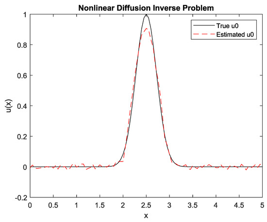
Figure 10.
Estimated
by GMRES spatio-temporal regularization with a preconditioner with
.
Figure 11 shows a comparison of the 3D simulation (noiseless) of the nonlinear diffusion equation with
, and the resulting constrained estimation surface for all the time interval
by considering the proposed GMRES spatio-temporal regularization with a preconditioner is shown.
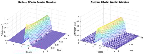
Figure 11.
Space-time dynamic simulation and constrained estimation surface of the nonlinear diffusion equation by considering the proposed GMRES spatio-temporal regularization with a preconditioner with
.
It can be seen from Figure 11 that the temporal constraint enforces that the estimation surface has soft transitions between the temporal samples.
An additional simulation is performed for
s and
. The simulation, the measurements, and the estimation are shown in Figure 12.
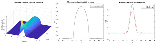
Figure 12.
Simulation, measurement, and estimation by using spatio-temporal Tikhonov with
and
with
s.
It is worth noting that since the value of T is increased, the value of
must also be increased in order to fulfil the CFL conditions:
Since the selected time step is
, the CFL condition is satisfied. In addition, it is worth noting that the estimation error for this case is 0.5562, and the number of iterations is 20. In comparison to the simulation of
, it can be seen that for this case it is harder to estimate the initial condition since the inverse problem becomes even more ill-conditioned.
4.2. Two-Dimensional Estimation Results
The forward problem is extended to the two-dimensional nonlinear diffusion equation with nonlinearity parameter
. The initial condition
is defined as a 2D Gaussian function centered in the middle of the spatial domain:
where the spatial domain is defined by
and
with
. The spatial discretization is performed using
grid points in each direction, which leads to step sizes
and
. The total simulation time is
, with
uniform time steps of size
. We now compute the CFL limit according to (9), by considering that
:
Since the selected time step is
, the CFL condition is satisfied.
The observed
with an additive noise of
is shown in Figure 13.
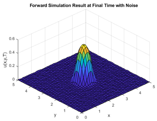
Figure 13.
Observed
for the 2D simulation.
The estimated
from observed
by using the GMRES with a preconditioner of the regularized spatio-temporal solution with
and
is shown in Figure 14.
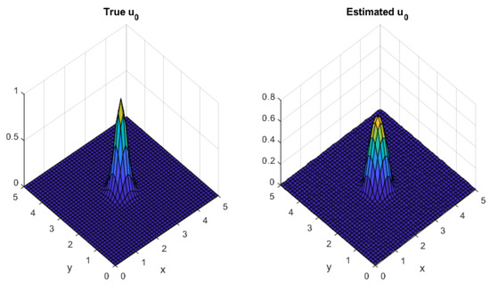
Figure 14.
Estimated
by GMRES spatio-temporal regularization with a preconditioner for the 2D simulation.
A comparison with the Tikhonov method with spatial constraints and regularization parameter of
is performed. As a result, Table 2 summarizes the performance of each method in terms of the estimation error for the 2D simulation.
Table 2.
Estimation error in 2D.
It can be seen from Table 2, the lowest estimation error is also achieved by the proposed approach, namely the spatio-temporal regularized Gauss–Newton method with GMRES and a preconditioner.
5. Conclusions
In this work, we proposed a dynamic inverse solution framework with spatio-temporal constraints for the nonlinear heat diffusion problem in both 1D and 2D, based on a regularized Gauss–Newton method integrated with Krylov subspaces and a preconditioner. The proposed approach was evaluated through numerical experiments and compared against classical methods, including Tikhonov regularization, and GMRES solvers with and without preconditioning, under both purely spatial and combined spatio-temporal regularization settings. The results consistently demonstrate that incorporating spatio-temporal constraints into the regularization significantly improves the accuracy of the estimated initial condition. Furthermore, the use of the Gauss–Newton method within a Krylov subspace framework, combined with an efficient Jacobian-based preconditioner, accelerates convergence and enhances numerical stability, particularly in the 2D case where problem size and complexity increase. Compared to the evaluated alternatives, the proposed method achieves lower estimation errors, especially under challenging conditions such as limited observations or high noise levels. These findings support the effectiveness of the proposed framework as a generalized and scalable solution strategy for nonlinear dynamic inverse problems governed by time-dependent partial differential equations.
Author Contributions
Conceptualization, E.G.; Methodology, L.F.A.-V. All authors have read and agreed to the published version of the manuscript.
Funding
This work is funded by Universidad Tecnológica de Pereira, Pereira, Colombia.
Data Availability Statement
The original contributions presented in the study are included in the article, further inquiries can be directed to the corresponding author.
Conflicts of Interest
The authors declare that there are no conflict of interest regarding the publication of this paper.
References
- Mueller, J.L.; Siltanen, S. Linear and Nonlinear Inverse Problems with Practical Applications; Society for Industrial and Applied Mathematics: Philadelphia, PA, USA, 2012. [Google Scholar] [CrossRef]
- Arridge, S.; Maass, P.; Öktem, O.; Schönlieb, C.B. Solving inverse problems using data-driven models. Acta Numer. 2019, 28, 1–174. [Google Scholar] [CrossRef]
- Kadioglu, S.; Ozugurlu, E. A Jacobian-Free Newton–Krylov Method to Solve Tumor Growth Problems with Effective Preconditioning Strategies. Appl. Sci. 2023, 13, 6579. [Google Scholar] [CrossRef]
- Jin, Q.N. On the iteratively regularized Gauss–Newton method for solving nonlinear ill-posed problems. Math. Comput. 2000, 69, 1603–1623. [Google Scholar] [CrossRef]
- Buccini, A.; de Alba, P.D.; Pes, F.; Reichel, L. An Efficient Implementation of the Gauss–Newton Method Via Generalized Krylov Subspaces. J. Sci. Comput. 2023, 97, 44. [Google Scholar] [CrossRef]
- Rajan, M.; Jose, J. An Efficient Discretization Scheme for Solving Nonlinear Ill-Posed Problems. Comput. Methods Appl. Math. 2024, 24, 173–184. [Google Scholar] [CrossRef]
- Jin, K.H.; McCann, M.T.; Froustey, E.; Unser, M. Deep convolutional neural network for inverse problems in imaging. IEEE Trans. Image Process. 2019, 26, 4509–4522. [Google Scholar] [CrossRef]
- Zhao, Y.; Xu, Y.; Zhang, L. Numerical methods for solving the inverse problem of 1D and 2D PT-symmetric potentials in the NLSE. Comput. Math. Appl. 2025, 183, 137–152. [Google Scholar] [CrossRef]
- Woodbury, K.; Najafi, H.; de Monte, F.; Beck, J. Inverse Heat Conduction Problems. In Inverse Heat Conduction; Chapter 1; John Wiley & Sons, Ltd.: Hoboken, NJ, USA, 2023; pp. 1–23. [Google Scholar] [CrossRef]
- Chang, C.W.; Liu, C.H.; Wang, C.C. Review of Computational Schemes in Inverse Heat Conduction Problems. Smart Sci. 2018, 6, 94–103. [Google Scholar] [CrossRef]
- Roy, A.D.; Dhiman, S. Solutions of one-dimensional inverse heat conduction problems: A review. Trans. Can. Soc. Mech. Eng. 2023, 47, 271–285. [Google Scholar] [CrossRef]
- Li, H.; Lei, J.; Liu, Q. An inversion approach for the inverse heat conduction problems. Int. J. Heat Mass Transf. 2012, 55, 4442–4452. [Google Scholar] [CrossRef]
- Dinmohammadi, A.; Jafarabadi, A. Inverse heat conduction problem with a nonlinear source term by a local strong form of meshless technique based on radial point interpolation method. Comput. Appl. Math. 2023, 42, 284. [Google Scholar] [CrossRef]
- Shidfar, A.; Karamali, G.; Damirchi, J. An inverse heat conduction problem with a nonlinear source term. Nonlinear Anal. Theory Methods Appl. 2006, 65, 615–621. [Google Scholar] [CrossRef]
- Liu, T.; Ouyang, D.; Guo, L.; Qiu, R.; Qi, Y.; Xie, W.; Ma, Q.; Liu, C. Combination of Multigrid with Constraint Data for Inverse Problem of Nonlinear Diffusion Equation. Mathematics 2023, 11, 2887. [Google Scholar] [CrossRef]
- Uyanna, O.; Najafi, H. A novel solution for inverse heat conduction problem in one-dimensional medium with moving boundary and temperature-dependent material properties. Int. J. Heat Mass Transf. 2022, 182, 122023. [Google Scholar] [CrossRef]
- Pacheco, C.; Lacerda, C.; Colaço, M. Automatic selection of regularization parameter in inverse heat conduction problems. Int. Commun. Heat Mass Transf. 2022, 139, 106403. [Google Scholar] [CrossRef]
- Ciofalo, M. Solution of an inverse heat conduction problem with third-type boundary conditions. Int. J. Therm. Sci. 2022, 175, 107466. [Google Scholar] [CrossRef]
- Vazquez, J.L. The Porous Medium Equation: Mathematical Theory; Oxford University Press: Oxford, UK, 2006. [Google Scholar]
- LeVeque, R.J. Finite Difference Methods for Ordinary and Partial Differential Equations: Steady-State and Time-Dependent Problems; SIAM: Philadelphia, PA, USA, 2007. [Google Scholar]
- Thomas, J.W. Numerical Partial Differential Equations: Finite Difference Methods; Springer: Berlin/Heidelberg, Germany, 1995. [Google Scholar]
- Strikwerda, J.C. Finite Difference Schemes and Partial Differential Equations; SIAM: Philadelphia, PA, USA, 2004. [Google Scholar]
- Min, T.; Geng, B.; Ren, J. Inverse estimation of the initial condition for the heat equation. Int. J. Pure Appl. Math. 2013, 82, 581–593. [Google Scholar] [CrossRef]
- Gazzola, S.; Hansen, P.C.; Nagy, J.G. IR Tools: A MATLAB package of iterative regularization methods and large-scale test problems. Numer. Algorithms 2019, 81, 773–811. [Google Scholar] [CrossRef]
- An, H.B.; Bai, Z.Z. A globally convergent Newton-GMRES method for large sparse systems of nonlinear equations. Appl. Numer. Math. 2007, 57, 235–252. [Google Scholar] [CrossRef]
- Quarteroni, A.; Sacco, R.; Saleri, F. Numerical Mathematics, 2nd ed.; Springer: Berlin/Heidelberg, Germany, 2007. [Google Scholar]


Disclaimer/Publisher’s Note: The statements, opinions and data contained in all publications are solely those of the individual author(s) and contributor(s) and not of MDPI and/or the editor(s). MDPI and/or the editor(s) disclaim responsibility for any injury to people or property resulting from any ideas, methods, instructions or products referred to in the content. |
© 2025 by the authors. Licensee MDPI, Basel, Switzerland. This article is an open access article distributed under the terms and conditions of the Creative Commons Attribution (CC BY) license (https://creativecommons.org/licenses/by/4.0/).