A Model Embedded with Development Patterns for Oilfield Production Forecasting

Abstract

Machine learning models that only use data for training and forecasting oilfield production have a sense of disconnection from the physical background, while embedding development patterns in them can enhance interpretability and even improve accuracy. In this paper, a novel multi-well production forecasting model embedded with decline curve analysis (DCA) is proposed, enabling the machine learning model to incorporate physical information. Moreover, an improved particle swarm optimization algorithm is proposed to optimize the hyperparameters in the loss function of the model. These hyperparameters determine the importance of the overall DCA and each module in training, which traditionally requires expert knowledge to determine. Simulation results based on the benchmark reservoir model show that the model has better forecasting ability and generalization performance compared to typical machine learning methods.

1. Introduction

In the area of petroleum engineering, production forecasting, generally referring to oil production forecasting, is an important stage [1], reflected in the optimization of production plans, reduction of recovery cycles, resource management, investment decisions, environmental sustainability, and the improvement of oilfield economic benefits. Commonly used forecasting methods include numerical simulation, physical modeling [2], decline curve analysis (DCA) methods [3], and machine learning. These methods have continuously emerged and improved over the history of reservoir development, and the reasons for their advancement include both accuracy and the requirement for rapid on-site deployment. Specifically, numerical simulation relies on reservoir simulation software, taking into account geological characteristics such as permeability and porosity of the oilfield, as well as fluid dynamics and other physical processes, for forecasting. However, reservoir simulation software incurs high computational costs, making it difficult to achieve fast and accurate decision-making. When it comes to physical modeling, the complexity, diversity, and heterogeneity of reservoirs make it difficult to establish a comprehensive physical model. Even worse, the limited understanding of underground structures also makes it more difficult to rely solely on physical models for forecasting. From a practical perspective, DCA methods based on mathematical statistics can provide engineers with quick assistance in on-site production forecasting, although the accuracy of these methods depends on engineers’ knowledge in determining key parameters. Therefore, with the current level of knowledge, other more flexible methods, such as machine learning or artificial intelligence combined with classical methods, may be more effective in coping with these uncertainties and improving the accuracy of subsurface structure prediction.

Neural networks, a branch of machine learning, have a wide range of applications in forecasting, performing well in performance testing of various machine learning methods including multivariate linear regression, artificial neural networks, gradient boost trees, adaptive boosting, and support vector regression [4,5]. Traditional methods such as autoregressive integral moving average (ARIMA) [6,7], random walk (RW) [8], generalized autoregressive conditional heteroskedasticity (GARCH) [9,10], and vector autoregression (VAR) [11] are effective in forecasting linearly correlated variables. Time series data in reality often exhibit nonlinear long sequence characteristics and are prone to unstable fixed points due to environmental interference and human recording errors. In this regard, ARIMA and VAR may exhibit low prediction accuracy due to strict requirements for data stability, RW may be difficult to achieve long-term prediction due to strong randomness, and GARCH may have inaccurate estimation of non-negative constraint model parameters that are easily violated. Overall, traditional methods lack the ability to capture complex dynamic relationship problems, manifested as insufficient accuracy and low efficiency. The limitations of traditional methods have given rise to numerous nonlinear artificial intelligence and deep learning methods that can be applied to time series forecasting tasks. For instance, artificial neural networks (ANNs) [12], support vector machines [13], and back propagation neural networks (BPNNs) are nonlinear methods and models that can be employed to address the inherent nonlinearity of time series [14].

Since production forecasting is not only related to the sequence at the current time but also to previous data, the information carried by earlier data will be lost if only the data at the most recent point in time is used. This type of time series forecasting problem gave rise to recurrent neural networks (RNN) [15]. 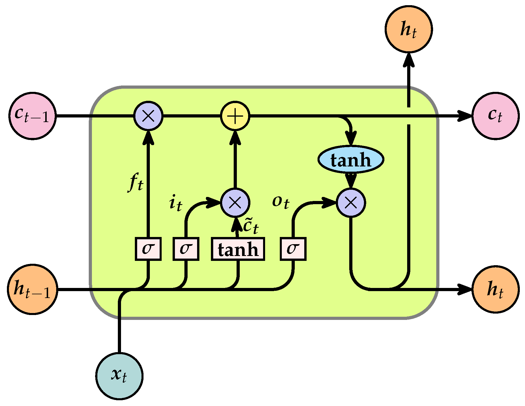In contrast to traditional ANNs, some of the connections between hidden units are refactored, which enables the neural structure to retain the memory of the most recent state, rendering it particularly well suited for the task of time series forecasting [16,17]. However, RNN suffers from gradient explosion and gradient vanishing, so an improved model based on RNN, called long short-term memory (LSTM), is proposed [18,19]. LSTM introduces a gating mechanism that can be viewed as a simulation of human memory. This mechanism allows the network to memorize useful information and discard useless information, thereby emulating the selective retention observed in human memory [20]. LSTM can be used to extract the data’s long- and short-term dependencies for the purpose of sequence forecasting.

In order to further improve the prediction effect of the model, it is necessary to optimize the hyperparameters in the neural network model. The optimization of hyperparameters represents a pivotal stage in the enhancement of the model’s performance. This study focuses on the optimization of hyperparameters within the network’s loss function, with the objective of optimizing the model’s generalization ability and overall performance. The more common hyperparameter optimization methods include stochastic optimization [21], gradient-based optimization [22], genetic algorithm optimization [23], particle swarm optimization [24], etc. The particle swarm optimization (PSO) algorithm [25] is a heuristic optimization algorithm that can achieve global optimization with fewer parameters. It is more widely used because of its excellent performance in terms of simplicity and ease of implementation, strong global search capability, parallelism, adaptability, and no gradient requirement. However, it also has the limitations of precocious convergence and sensitive parameter selection. In order to overcome the shortcomings of the algorithm, scholars have improved the particle swarm algorithm in several aspects, such as convergence improvement, parameter adaptation, mixing, and fusion. The canonical PSO algorithm tends to fall into local optimum due to lack of diversity, improper parameter selection, complexity of the search space, etc. Consequently, an improved PSO algorithm based on individual difference evolution [26] adopts an enhanced restart strategy to regenerate the corresponding particles, thereby enhancing population diversity. The multi-population particle swarm optimization algorithm [27] adopts various swarm strategies that are considered to have the potential to improve population diversity. Besides, the algorithm cooperates with the dynamic subpopulation number strategy, subpopulation recombination strategy, and purposeful detection strategy. The stretching technique in PSO can also improve the performance of the algorithm [28]. Subsequently, the pyramid particle swarm optimization (PPSO) algorithm [29] incorporating the pyramid concept combines novel competitive and cooperative strategies. A chaotic map has been introduced into the whale optimization algorithm [30], increasing the diversity of the population and accelerating the convergence of the algorithm.

While machine learning algorithms have achieved considerable success, they remain imperfect, such as in their lack of interpretability. Lack of interpretability refers to the difficulty for humans to intuitively understand or explain the decision-making process and internal mechanisms of neural networks using simple logic. In engineering fields such as reservoir development, lack of interpretability typically refers to models that are only based on data modeling without fully considering expert knowledge and physical constraints, which may lead to low modeling efficiency [31]. To solve the problem of poor interpretability of neural network models, a joint learning model that incorporates both physical information and neural networks has been developed. This approach makes use of the structural information inherent to physical equations, as well as the learning capabilities of neural networks, with the aim of enhancing the accuracy, generalization capacity, and interpretability of the model. The neural network framework based on physical information has a wide range of applications in power system applications [32], solving partial differential equations [33,34], fluid dynamics [35], turbulence prediction [36] and other areas. Numerical experiments have shown that the joint learning model of physical information and neural networks has better predictability, reliability, and generalization ability. However, for oilfield production forecasting, the current model faces some challenges in practical applications. The physical constraints used in the models require real-time access to data on saturation or pressure changes, which is not easy to obtain in practical oilfield applications.

It is worthwhile to highlight several aspects of the contributions developed by this study.

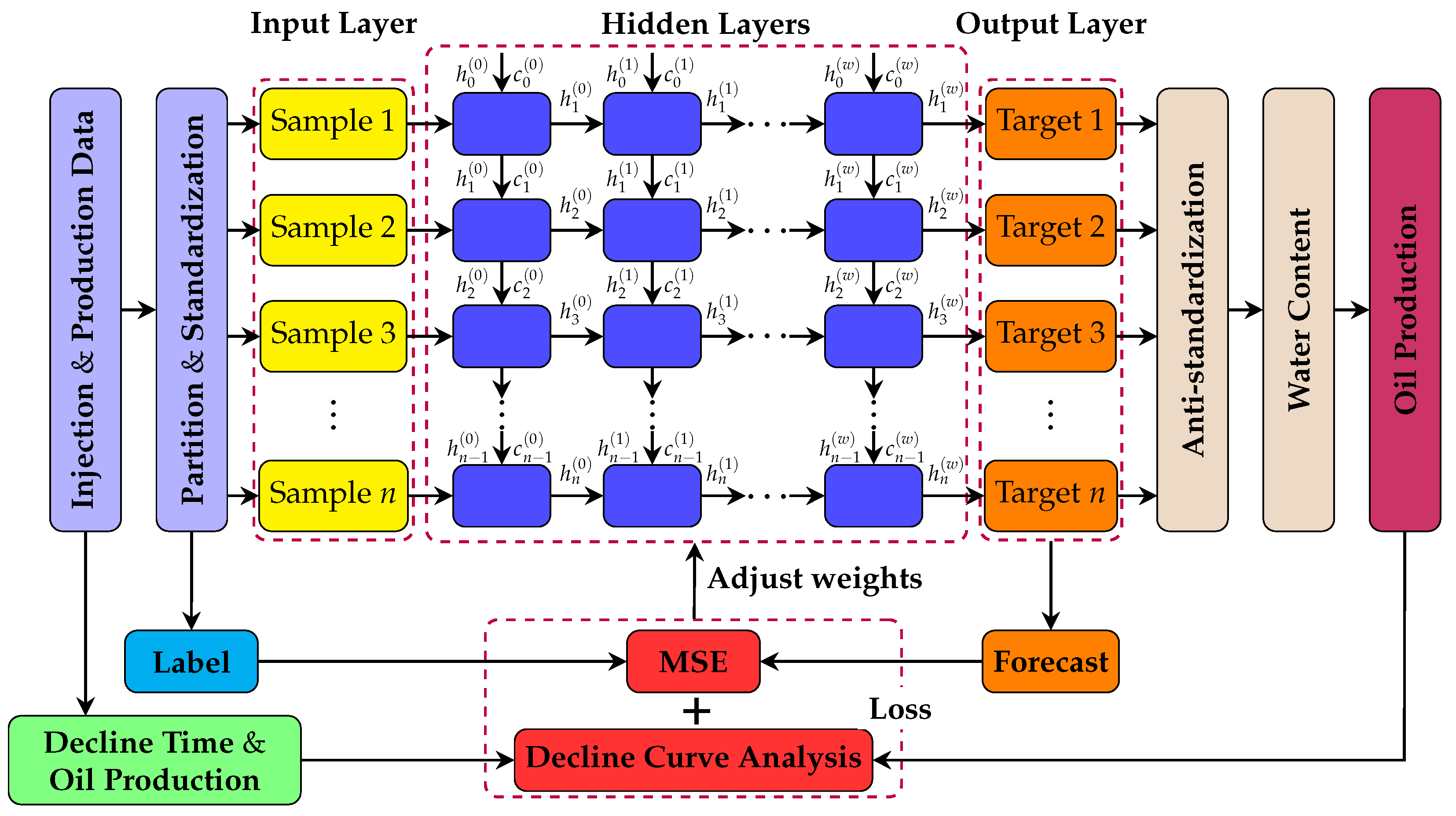
• A machine-learning multi-well production forecasting model embedded with the production development pattern is proposed. Specifically, this study aims to provide a more comprehensive and dynamic analysis method to improve the development efficiency of water-driven oilfields by introducing the production decline pattern as a physical constraint of the neural network. In addition, compared with the single-well production forecasting model, the multi-well model is more general and more adaptable to the oilfield.
• The model is constructed entirely on the basis of real-time acquisition of dynamic oilfield development data by monitoring and recording key parameters during actual operations and production. This universal approach ensures the practicality of the model, as it directly reflects the real situation of oilfield development.
• An improved PSO algorithm is proposed to optimize the hyperparameters in the loss function of the neural network to find the optimal setting instead of expert knowledge, thereby enhancing the performance of the model. During the optimization process, particles are updated by PSO with pyramid topology. The learning factor is adaptive, a particle iteration stagnation value strategy is introduced to ensure population diversity, and a chaotic map is used to initialize the initial population.

2. Methodology

In this section, a multi-well production forecasting model is proposed to achieve the research objective of this work presented in Section 2.1. Firstly, the principle and application of DCA are introduced in Section 2.2.1. Then, the theoretical basis of the LSTM and PSO algorithms are exhibited in Section 2.2.2 and Section 2.2.3, respectively. The construction process of the forecasting model is elaborated in Section 2.3, including the embedding approach of DCA and the data format. Subsequently, the design process of the novel evolutionary algorithm proposed in this paper, which is not only put forward as an independent innovation but also serves as a tool for optimizing the embedding structure of DCA, is presented in Section 2.4.

2.1. Research Objective

This study aims to establish a practical machine learning model for forecasting oil production based on real-time dynamic data of oilfield development and embedded with development patterns in the area of petroleum engineering.

2.2. Preliminaries

2.2.1. Decline Curve Analysis

In terms of the whole process of oilfield development, any oilfield should go through three stages of production increase, production stability and production decline, as shown in Figure 1.

The DCA method is a kind of mathematical statistics method for forecasting and analyzing reservoir performance of oilfields that are already in the production decline stage, which is the dashed box area marked as III in Figure 1. The Arps DCA [3] method is the most widely recognized theory to describe the production decline pattern, showing the dynamic change of oil well production with time.

2.2.2. Long Short-Term Memory

The core structure of LSTM consists of a memory cell and three major gating mechanisms, among which the memory cell is the key carrier for achieving long-term dependence, and gating mechanism is the foundation for dynamically regulating information flow. The memory cell illustration is shown in Figure 2, revealing that it has three inputs and two outputs at time t. The input consists of the input value at the current time $x_t$, the output value at the previous time $h_{t-1}$, and the cell state at the previous time $c_{t-1}$. The outputs consist of the current time $s_t$ and the cell state at the current time $c_t$. The specific gate structure workflow of LSTM is as follows [18,37].

Firstly, the forget gate $f_t$ is used to determine which information to discard from the unit state, defined as

$$f_t=\sigma (U_f{x}_t+W_f{h}_{t-1}+b_f).$$

(1)

Notably, the output values of the forget gate, as well as the following input and output gates, are in the range of $[0,1]$. Among them, 0 means complete forgotten (closed), which does not allow any information to pass. One means complete kept (open), which allows all information to pass.

Secondly, the input gate $i_t$ is used to determine which new information will be stored in the cell state, defined as

$$i_t=\sigma (U_i{x}_t+W_i{h}_{t-1}+b_i).$$

(2)

Then, calculate the value of the memory cells $c_t$ by

$$c_t=f_t\otimes c_{t-1}+i_t\otimes {\tilde{c}}_t,$$

(3)

where ${\tilde{c}}_t$ is the candidate cell defined as

$${\tilde{c}}_t=tanh(U_c{x}_t+W_c{h}_{t-1}+b_c).$$

(4)

Finally, the output information is determined by the output gate $o_t$, while $h_t$ is controlled within the range of $(-1,1)$ using the tanh function.

$$\begin{array}{cc}\hfill o_t& =\sigma (U_o{x}_t+W_o{h}_{t-1}+b_o),\hfill \\ \hfill h_t& =o_t\otimes tanh{c}_t.\hfill \end{array}$$

(5)

Among all the above equations, $\sigma (·)$ denotes sigmoid function, $W_f,W_i,W_c,W_o$ denote parameter matrices, $U_f,U_i,U_c,U_o$ denote input weight matrices, and $b_f,b_i,b_c,b_o$ denote bias vectors.

2.2.3. Pyramid Particle Swarm Optimization

The PSO algorithm [25] is a population-based optimization algorithm, inspired by the simulation of bird foraging behavior. Each particle represents a possible solution in the particle swarm. Within a given search area, the particles continuously adjust their speed and position by comparing the individual extremes and global extremes to perform the optimization search until an optimal solution is found that satisfies the termination conditions. The formula is as follows:

$$\begin{array}{c}\hfill \left\{\begin{array}{c}{V}_{i,j}^{t+1}=\omega V_{i,j}^t+c_1{r}_1(X_{\mathrm{pbest},j}^t-X_{i,j}^t)+c_2{r}_2(X_{\mathrm{gbest},j}^t-X_{i,j}^t),\hfill \\ X_{i,j}^{t+1}=X_{i,j}^t+V_{i,j}^{t+1},\hfill \end{array}\right.\end{array}$$

(6)

where t is the number of iterations, $V_{i,j}^{t+1}$,$X_{i,j}^{t+1}$ are the velocity and position of particle i in dimension j at iteration $t+1$, respectively, $\omega$ is the inertia weight, $c_1$ and $c_2$ are the learning factors, $X_{\mathrm{pbest},j}^t$ is the individual extremum point in the t-th iteration of the particle swarm, $X_{\mathrm{gbest},j}^t$ is the global extremum of the particle swarm, and $r_1$ and $r_2$ are the random numbers obeying uniform distribution in the interval [0, 1].

In PPSO, a variant algorithm of PSO, a pyramid structure is introduced to organize the particle swarm, where two random particles at one level are paired and divided into a loser and a winner [29]. The loser and the winner evolve according to different rules. PPSO divides the search space into several levels, each corresponding to a particle swarm, thus realizing multilevel search. These particle swarms are organized in the form of a pyramid, with the number of particles gradually decreasing from the bottom to the top. The particles in the top layer can guide all the particles in the pyramid, while the particles in the other layers can only guide the particles in the layer below. This topology is able to distribute the responsibility more evenly than the traditional topology. The pyramid structure is shown in Figure 3, wherein each generation, the particles are sorted in ascending order according to their fitness.

Competition and cooperation affect the performance and results of evolutionary computation algorithms. To enhance diversity, PPSO introduces more competitive strategies. One competitive strategy is the global competitive strategy, where all particles are sorted to determine which layer of the pyramid they are in when the pyramid is constructed. The other competitive strategy is the local competitive strategy, where particles in each layer except the top layer are randomly paired separately into two groups, i.e., winners and losers. Winners can learn from particles at higher levels, while losers can only learn from winners at the same level. For cooperation, PPSO uses a cooperation strategy in which each particle has the opportunity to cooperate with several better particles in addition to its own best particle. Mathematically, the losers and the winners at the i-th layer update their velocities and positions according to Equation (7) and Equation (8), respectively.

$$\begin{array}{c}\hfill \left\{\begin{array}{c}{V}_{L_{i,j}}^{t+1}=r_1{V}_{L_{i,j}}^t+r_2(X_{L_{\mathrm{pbest},j}}^t-X_{L_{i,j}}^t)+r_3(X_{W_{i,j}}^t-X_{L_{i,j}}^t),\hfill \\ X_{L_{i,j}}^{t+1}=X_{L_{i,j}}^t+V_{L_{i,j}}^{t+1},\hfill \end{array}\right.\end{array}$$

(7)

$$\begin{array}{c}\hfill \left\{\begin{array}{cc}{V}_{W_{i,j}}^{t+1}=\hfill & r_4{V}_{W_{i,j}}^t+r_5(X_{W_{\mathrm{pbest},j}}^t-X_{W_{i,j}}^t)+\hfill \\ \hfill & r_6(X_{P_{i-1,k}}^t-X_{W_{i,j}}^t)+\rho r_7(X_{P_{1,\kappa }}^t-X_{W_{i,j}}^t),\hfill \\ X_{W_{i,j}}^{t+1}=\hfill & X_{W_{i,j}}^t+V_{W_{i,j}}^{t+1},\hfill \end{array}\right.\end{array}$$

(8)

where $r_i(i=1,2,\dots ,7)$ is a random value obeying a uniform distribution in the range $(0,1)$; $\rho$ is a constant controlling the magnitude of the influence of a particle in the top layer on the current particle; $P_{i,j}$, $L_{i,j}$, and $W_{i,j}$ respectively denote the j-th particle among all the particles, losers, and winners in the i-th layer; $X^t$, $V^t$, and $X_{\mathrm{pbest}}^t$ respectively denote the position, velocity, and historical optimum of the particle in the t-th generation; k and $\kappa$ are random positive integers not larger than ${\delta }_{i-1}$ and ${\delta }_1$. Note that ${\delta }_i$ indicates the presence of $\delta$ particles in the i-th layer. For particles at the top level, the loser also uses the update strategy of Equation (8), while the winner will be passed directly to the next generation.

In summary, the key advantages of the PPSO algorithm over the well-known PSO algorithm can be summarized in five points.

• Multi-layer search architecture enhances global and local optimization capabilities.
• Pyramid topology structure improves information flow diversity.
• Competition-cooperation strategies elevate particle evolutionary efficiency.
• Balanced responsibility allocation prevents premature convergence.
• Fitness-based sorting optimizes particle update strategies.

2.3. Lstm Embedded with DCA

Embedding a priori knowledge of development patterns and practical theories into neural networks can guide the training process, speed up the convergence of the model, and improve the interpretability [38]. Under this guidance, LSTM embedded with DCA (LSTM-DCA) is proposed in this paper.

2.3.1. Loss Function During Training

Typically, the loss function used by a neural network during training is measured by feeding samples into the network and calculating the mean square error (MSE) between the network output and the actual target value. It can be expressed as

$$L_{\mathrm{data}}\left(\theta \right)={\displaystyle \frac{1}{N}}{\sum }_{i=1}^N{(y_i-f_{\theta }\left(x_i\right))}^2,$$

(9)

where $L\left(\theta \right)$ is the loss function, $\theta$ denotes the parameters of the neural network, N is the number of samples, $x_i$ is the input of the i-th sample, $y_i$ is the actual target value, and $f_{\theta }\left(x_i\right)$ is the forecasting output of the neural network.

In this paper, the Arps DCA method is introduced into the loss function, with one of its commonly used basic forms being

$$\begin{array}{c}\hfill Q_t=\left\{\begin{array}{cc}{Q}_0{e}^{-d_{0}t},\hfill & \eta =0,\hfill \\ Q_0{(1+\eta d_{0}t)}^{-{\displaystyle \frac{1}{n}}},\hfill & 0<\eta <1,\hfill \\ Q_0{(1+d_{0}t)}^{-1},\hfill & \eta =1,\hfill \end{array}\right.\end{array}$$

(10)

where $Q_t$ is the oil production at time t, $Q_0$ is the oil production at the initial decline moment, $d_0$ is the initial decline rate, and $\eta$ is the decline index with a domain of $[0, 1]$. Depending on the value of $\eta$, the Arps DCA method can be summarized as exponential decline $(\eta =0)$, hyperbolic decline $(0<\eta <1)$, and harmonic decline $(\eta =1)$. And it is not difficult to see that exponential and harmonic types are special cases of hyperbolic type. Since there is no absolute order in which the three decline types appear [3,39], the loss function needs to consider three types at the same time by setting a coefficient to limit the importance of each type.

Subsequently, the loss terms of exponential, hyperbolic, and harmonic types are respectively given as Equations (11)–(13).

$$L_{\mathrm{e}}\left(\theta \right)=\left|{\displaystyle \frac{{\widehat{Q}}_t}{Q_0}}-e^{-d_{0}t}\right|,$$

(11)

$$L_{\mathrm{b}}\left(\theta \right)=\left|{\displaystyle \frac{{\widehat{Q}}_t}{Q_0}}-{(1+\eta d_{0}t)}^{-{\displaystyle \frac{1}{\eta }}}\right|,$$

(12)

$$L_{\mathrm{m}}\left(\theta \right)=\left|{\displaystyle \frac{{\widehat{Q}}_t}{Q_0}}-{(1+d_{0}t)}^{-1}\right|,$$

(13)

where ${\widehat{Q}}_t$ is the oil production obtained based on machine learning forecasting results.

It is worth noting that in equations Equations (11)–(13), $\eta$ and $d_0$ are unknown parameters to be determined. In fact, from the above analysis, it can be seen that the values of $\eta$ and $d_0$ determine the specific expression of Equation (10) of the Arps DCA method. Traditionally, the trial and error method can be used to determine $\eta$ and $d_0$, which is given by

$${\left({\displaystyle \frac{Q_0}{Q}}\right)}^{\eta }=1+\eta d_{0}t.$$

(14)

When $\eta$ takes the appropriate value, and ${(Q_0/Q)}^{\eta }$ is linearly related to t. Thus $d_0$ can be calculated by dividing the slope by $\eta$.

In this work, machine learning methods are employed to solve for $\eta$ and $d_0$ based on Equation (14). Firstly, according to the change of water content, the initial decline time can be determined so as to obtain the corresponding initial decline production. Specifically, based on the application experience of DCA, when the total water content of the oilfield is about 70%, the production enters the decline stage. Therefore, in this work, the corresponding production when the total water content of the oilfield is 70% is selected as the initial decline production $Q_0$.

Secondly, in order to ensure accuracy, production data of 24 months after the initial decline time is selected to fit Equation (14). In the $[0.01, 0.99]$ range content, 99 numbers are linearly generated as a value library for $\eta$. Using R-squared (${\mathrm{R}}^2$) as an evaluation criterion, by traversing the value library of $\eta$, the number that can make the left and right sides of Equation (14) the closest, that is, the number with the largest ${\mathrm{R}}^2$, is selected as the determined value of $\eta$. Moreover, ${\mathrm{R}}^2$ is defined as

$${\mathrm{R}}^2=1-{\displaystyle \frac{{\sum }_{i=1}^N{(y_i-f\left(x_i\right))}^2}{{\sum }_{i=1}^N{(y_i-\overline{y_i})}^2}},$$

(15)

where $f\left(x_i\right)$ is the fitting value, $y_i$ and $\overline{y_i}$ are the target data value and its average, respectively.

Therefore, the total loss function of the model is defined as

$$L\left(\theta \right)={\lambda }_{\mathrm{data}}{L}_{\mathrm{data}}+{\lambda }_{\mathrm{phy}}({\lambda }_{\mathrm{e}}{L}_{\mathrm{e}}+{\lambda }_{\mathrm{b}}{L}_{\mathrm{b}}+{\lambda }_{\mathrm{m}}{L}_{\mathrm{m}}),$$

(16)

where ${\lambda }_{\mathrm{data}}+{\lambda }_{\mathrm{phy}}=1$ and ${\lambda }_{\mathrm{e}}+{\lambda }_{\mathrm{b}}+{\lambda }_{\mathrm{m}}=1$, all of which are adjustable coefficients. In the data experiments, an improved particle swarm algorithm is adopted to determine the individual coefficients.

With the above way, DCA is embedded in the neural network of the data forecasting, making it interpretable.

2.3.2. Data Format

Given that the model presented in this paper is designed for practical field deployment, the features required for network training must be derived solely from the production data accessible on-site. These primarily encompass monthly production reports, wellbore permeability, reservoir thickness, total recoverable reserves, well depth, reservoir boundaries, pump efficiency, and casing pressure. Among these, structural parameters like well depth and boundaries, along with operational metrics such as pump efficiency and casing pressure, typically remain stable throughout the development process. Consequently, within the scope of this study, these parameters are treated as constants. The data formatting of the model is as follows.

Input Features

• Production and injection rates. The flow dynamics of fluid (oil and water) within the reservoir are governed by the liquid production rate (${\mathrm{m}}^3$/d) of production wells and the water injection rate (${\mathrm{m}}^3$/d) of injection wells. These rates exert a substantial influence on parameters such as pressure distribution and residual oil saturation. To enhance the machine learning model’s ability to discern between production and injection wells, a convention has been adopted in this study wherein the liquid production rate is denoted by a negative value and the water injection rate by a positive one.
• High-order features [40]. During feature engineering, high-order features, which are computed through the combination of existing features [41], have the potential to augment the efficacy of machine learning models. Given the possible nonlinear and complex relationships between reservoir data attributes, this study starts from Equation (17) [42] for reservoir production in water injection development scenarios.

  $$Q^{\mathrm{l}}={\displaystyle \frac{0.543kh\Delta p}{\mu ln{\displaystyle \frac{r_{\mathrm{e}}}{r_{\mathrm{w}}}}}},$$

  (17)

  where $Q^{\mathrm{l}}$ represents monthly liquid production (${\mathrm{m}}^3$/mth), k represents absolute permeability ($\mu$${\mathrm{m}}^2$), h represents reservoir thickness (cm), $\Delta p$ represents the production pressure difference (${10}^5$ Pa), $\mu$ represents the viscosity (mPa·s), $r_{\mathrm{e}}$ represents the supply radius (cm), and $r_{\mathrm{w}}$ represents oil well radius (cm), respectively. As $\mu$, $r_{\mathrm{e}}$, and $r_{\mathrm{w}}$ are typically treated as constants during the production process, while $\Delta p$ is exceedingly difficult to acquire from on-site data, $Q^{\mathrm{l}}$, k, and h are selected for the construction of a higher-order feature $q^{\mathrm{phy}}$ [40].

  $$q_i^{\mathrm{phy}}={\displaystyle \frac{Q_i^{\mathrm{l}}}{k_i·h_i·\Delta t_i}},$$

  (18)

  where $Q_i^{\mathrm{l}}$, $k_i$, $h_i$, and $\Delta t_i$ represent the monthly liquid production, well point permeability, well point reservoir thickness, and monthly production time of the i-th production well, respectively.

Output Target

To avoid overfitting of neural networks and failure of data anti-standardization, water content is used as the target value of the model. The adequacy of its rationale has been amply demonstrated [40]. Furthermore, the ultimate target oil production in actual applications can be obtained through Equation (19)

$$Q=Q^{\mathrm{l}}(1-f_{\mathrm{w}}),$$

(19)

where $f_{\mathrm{w}}$ represent water content.

Partition

The real scenario targeted by this study is to forecast future production dynamics using past development data under fixed well location conditions. The obvious limitation is that only one production history that changes over time is presented to engineers. Therefore, for a set of production data totaling N months, it is necessary to model the production dynamics for the next $N-M$ months based on the data from the first M months. According to the training process of the neural network, the data from the first M months comprise the training set, and the data from the last $N-M$ months comprise the testing set.

Sample Generation

Due to the time delay characteristic inherent in reservoir development, the water injection volume and liquid production volume in the preceding few months will also influence the oil production volume in the current month. To implement this design and meet the data structure requirements for the input of LSTM, the sliding window method is employed to construct training samples, as detailed in Figure 4. Furthermore, the core mechanistic advantage of LSTM, that is, the output of the previous time step serving as the input for the next time step, effectively addresses the time delay requirements of reservoir development.

Data Alignment

For an oilfield with i producing wells ($P_1$, $P_2$, …, $P_i$) and j injecting wells ($I_1$, $I_2$, …, $I_j$), the input and output data formats of the neural network are as illustrated in

Table 1. Input and output data alignment for neural network training with a sliding window length of 3.

Input			Output
Liquid Production Rate	Water Injection Rate	High Order Feature	Water Content
of${\mathbf{P}}_{\mathbf{1}}$,${\mathbf{P}}_{\mathbf{2}}$,… ,${\mathbf{P}}_{\mathit{i}}$.	of${\mathbf{I}}_{\mathbf{1}}$,${\mathbf{I}}_{\mathbf{2}}$, …,${\mathbf{I}}_{\mathit{j}}$.	of${\mathbf{P}}_{\mathbf{1}}$, ${\mathbf{P}}_{\mathbf{2}}$, …,${\mathbf{P}}_{\mathit{i}}$.	of${\mathbf{P}}_{\mathbf{1}}$,${\mathbf{P}}_{\mathbf{2}}$, …,${\mathbf{P}}_{\mathit{i}}$.
(${\mathbf{m}}^{\mathbf{3}}$/d)	(${\mathbf{m}}^{\mathbf{3}}$/d)	(Dimensionless)	(Dimensionless, [0, 1])
1st month	1st month	1st month	-
2nd month	2nd month	2nd month	-
3rd month	3rd month	3rd month	3rd month
⋮	⋮	⋮	⋮
n-th month	n-th month	n-th month	n-th month

. Combining this with Figure 4, it can be seen that if the sliding window length is set to 3, the data for the first two months in the output will be omitted. Consequently, the water content of the third month is the initial value that the model will forecast.

2.3.3. Model Structure

The learning and training process of the LSTM model consists of the following three steps.

• The forward computes the output value of each neuron, i.e., the values of the five vectors $f_t$, $i_t$, $c_t$, $o_t$, $h_t$.
• Backpropagation calculates the value of the error term for each neuron. As with recurrent neural networks, the backpropagation of the LSTM error term consists of two directions: backpropagation along time and propagation of the error term to the previous layer, where the former is specifically expressed as calculating the error term at each time starting from the current time t.
• The gradient of each weight is calculated based on the corresponding error term. And the Adam algorithm is used to optimize each trainable parameter, which adaptively adjusts the learning rate.

Based on the analysis in the previous section, the network loss function is updated by Equation (16). The model structure and training process is shown in Figure 5.

2.4. Adaptive Pyramidal Particle Swarm Optimization Based on Chaotic Map

To further enhance the performance of PPSO, this study introduces targeted improvements aimed at augmenting particle self-learning capabilities and population diversity. Consequently, an adaptive pyramidal particle swarm optimization algorithm based on a chaotic map (CAPPSO) is proposed.

2.4.1. Adaptive Learning Factor

The learning factor plays an important role in particle swarm optimization algorithms, influencing the speed and direction of particle movement in the search space. Specifically, the learning factor serves to balance the trade-offs between exploration and exploitation of the particles and is dynamically adapted to fit different optimization problems and search methods, which in turn affects the algorithm’s search performance and convergence speed of the algorithm. The pyramid structure is often used in organizational management to describe a hierarchical structure, with each layer representing a different level of management. The need for each layer to learn from those who are better, as well as the need for continuous learning themselves, is one of the key factors in building an efficient organization and sustaining growth. The particles learn from the better particles to obtain the information of the global optimal solution, and at the same time, it is more necessary to continuously optimize their own search strategy through their own learning and adaptation. As the number of iterations increases, the particles accumulate more search experience and historical information, so increasing the individual learning factor can make the particles more confident in their own experience and more active in adjusting their own motion strategies and parameters to guide the search direction, thus accelerating the convergence to a more optimal solution.

The adaptive learning factor designed in this paper is defined as

$$\xi \left(t\right)=1.0+sin({\displaystyle \frac{\pi }{2}}·{\displaystyle \frac{t}{T_{\max }}}),$$

(20)

where t is the current number of iterations and $T_{\max }$ is the maximum number of iterations of the algorithm. The individual learning factor increases with the number of iterations.

As a result, Equation (7) and Equation (8) have been improved to Equation (21) and Equation (22). The losers and winners at the i-th layer update their velocities and positions according to Equation (21) and Equation (22), respectively.

$$\begin{array}{c}\hfill \left\{\begin{array}{c}{V}_{L_{i,j}}^{t+1}=r_1{V}_{L_{i,j}}^t+\xi \left(t\right)r_2(X_{L_{\mathrm{pbest},j}}^t-X_{L_{i,j}}^t)+r_3(X_{W_{i,j}}^t-X_{L_{i,j}}^t),\hfill \\ X_{L_{i,j}}^{t+1}=X_{L_{i,j}}^t+V_{L_{i,j}}^{t+1},\hfill \end{array}\right.\end{array}$$

(21)

$$\begin{array}{c}\hfill \left\{\begin{array}{cc}{V}_{W_{i,j}}^{t+1}=\hfill & r_4{V}_{W_{i,j}}^t+\xi \left(t\right)r_5(X_{W_{\mathrm{pbest},j}}^t-X_{W_{i,j}}^t)+\hfill \\ \hfill & r_6(X_{P_{i-1,k}}^t-X_{W_{i,j}}^t)+\rho r_7(X_{P_{1,\kappa }}^t-X_{W_{i,j}}^t),\hfill \\ X_{W_{i,j}}^{t+1}=\hfill & X_{W_{i,j}}^t+V_{W_{i,j}}^{t+1}.\hfill \end{array}\right.\end{array}$$

(22)

2.4.2. Iterative Stagnation Value

Population diversity is very important in PSO, as it helps to maintain the global exploration capability of the algorithm. The diversity of a population can be measured in a number of ways, such as by particle distribution, which is commonly used. If the particles are widely distributed, the diversity is high. Another indicator is the variability between individuals, both in terms of position and velocity. If all particles move in similar directions, the diversity decreases, which can cause the algorithm to fall into a local optimum solution.

In this paper, the concept of particle iterative stagnation value $\zeta$ is proposed to solve this issue. When the algorithm is iteratively solving for the optimal value, if the global extreme value of the particle swarm has not been updated and changed for $\zeta$ times in a row, $\Phi$ particles among all particles are randomly selected to re-update the particle position, which is given by

$$X_{\mathrm{new}}={\tau }_1·X_{\phi }+{\tau }_2·X_{\mathrm{pbest}},\phi =1,2,\dots ,\Phi .$$

(23)

Among them, $X_{\mathrm{new}}$ and $X_{\mathrm{pbest}}$ respectively represent the new candidate position and historical optimal position of particle $\phi$; ${\tau }_1$ and ${\tau }_2$ are both random numbers within [0, 1].

2.4.3. Population Initialization

Population initialization, as the starting point of the algorithm, has a crucial impact on the performance and results of the algorithm. A good population initialization strategy can help the algorithm find a good solution faster, while a bad initialization strategy can cause the algorithm to fall into a locally optimal solution.

In this paper, the chaos function for population initialization is introduced to enhance the randomness and diversity of particles. Ten commonly used chaotic map algorithms include tent mapping [43] ($\mu =0.45$), logistic map [43] ($\lambda =2$), cubic map [44] ($\rho =1$), Chebyshev map [43] ($k=4$), piecewise map [44] ($d=0.4$), sinusoidal map [44] ($\alpha =2$), sine map [43] ($\alpha =2$), iterative chaotic map with infinite collapses mapping [43] ($\alpha =2$), circle map [43] ($\Omega =0.5,K=0.5$), and Bernoulli map [43] ($\lambda =0.4$). In this algorithm, one of the chaotic functions is randomly selected to execute the algorithm.

The entire algorithm of CAPPSO includes the use of a chaotic map to initialize the population, the establishment of the pyramid structure and the implementation of particle stratification, the competition and cooperation from the bottom to the second level, the cooperation of the losers in the top level, the particle iteration stagnation strategy, and the particle adaptive value evaluation in six parts. The iteration is terminated when the total number of evaluations reaches the maximal times of fitness evaluation. CAPPSO makes the particles adaptive to adjust their own updating strategies and speed up the convergence of the algorithm by strengthening their own learning to improve the algorithm’s ability to search locally. At the same time, it adopts a chaotic map to initialize the population and introduces the particle iteration stagnation condition of the particles to increase the diversity of the population so as to better realize the global search.

3. Experiments

In this section, the Egg model with fixed wells is used to evaluate the proposed forecasting model. Root Mean Square Error (RMSE) and $R^2$ are selected as the evaluation criteria for the instance validation, with the former defined as

$$\mathrm{RMSE}=\sqrt{{\displaystyle \frac{1}{N}}\sum _{i=1}^N{(y_i-f\left(x_i\right))}^2},$$

(24)

where $f\left(x_i\right)$ is the forecasting value of the neural network, and $y_i$ is the actual data value. Moreover, the standard deviation (SD) of the error between the forecasting value and the actual value is utilized to quantify variability, with its computational formula given by

$$\mathrm{SD}=\sqrt{{\displaystyle \frac{{\sum }_{i=1}^N{({ϵ}_i-\overline{ϵ})}^2}{N-1}}},$$

(25)

where ${ϵ}_i=y_i-f\left(x_i\right)$ and $\overline{ϵ}$ represents the mean value.

3.1. Egg Model

The Egg model is a three-dimensional two-phase (oil and water) benchmark model for reservoir simulation [45], which is a fluvial sedimentary facies reservoir. With its complex geological structure and inhomogeneous permeability and porosity distribution, it is widely used to validate the accuracy of reservoir simulation software, compare algorithmic performance, and develop new techniques.

The Egg model includes eight injection wells and four production wells, and the model structure is shown in Figure 6. The production cycle is (360 × 20) days, and the development dynamics data are recorded on a monthly basis, so there are 240 sets of monthly oil production data.

3.2. LSTM-DCA

In this section, the forecasting results of LSTM-DCA on the Egg model are discussed. In addition, a comparison was performed with three forecasting models, which are BPNN, convolutional neural network (CNN) and LSTM.

3.2.1. Parameters Setting

The numerical simulation software Eclipse (version 2018.1), developed by Schlumberger, is employed to generate data while accounting for the restrictions derived from on-site data acquisition capabilities. In particular, it is worth noting that the DCA method represents the regular characteristics of oil production during the high water content period. Moreover, data from the water-free oil production period and the low water content period can negatively affect the training of the model. Therefore, data from individual wells before the water content reaches approximately 70% was removed to ensure that the network takes advantage of DCA as much as possible. Thus, the accuracy of forecasting can be improved during and after the high water content period.

Based on the analysis of Arps DCA and production experience, the loss function parameters ${\lambda }_{\mathrm{data}}$, ${\lambda }_{\mathrm{phy}}$, ${\lambda }_{\mathrm{e}}$, ${\lambda }_{\mathrm{b}}$ and ${\lambda }_{\mathrm{m}}$ are set to 0.7, 0.3, 0.15, 0.7, and 0.15, respectively. The machine learning model is trained for 400 epochs at an initial learning rate of 0.001.

The implementation of the machine learning model uses Python 3.10.9 with Pytorch 1.12.1. And the training platform is NVIDIA (NVIDIA Corporation, Santa Clara, California, USA) GTX TITAN X with 12 GB video memory. In addition, to reduce the effect of randomness, we perform 10 independent runs for all experimental results. Each experiment, including data processing operations, takes about 350 seconds.

3.2.2. Results and Analysis

In actual development, production data for the decline stage is usually not a smooth curve but a zigzag decline. Under this background, the production forecasting results of BPNN, CNN, LSTM, and LSTM-DCA over the entire dataset are shown in Figure 7. It is not difficult to see that apart from CNN, the other three models have very small differences on the training set. Figure 8 and

Table 2. Comparison of forecasting performance between BPNN, CNN, LSTM, and LSTM-DCA on the testing set.

a Average ${\mathrm{R}}^2$
Well	BPNN	CNN	LSTM	LSTM-DCA
PRO-1	0.7080	0.7249	0.7392	0.8075
PRO-2	0.7890	0.8120	0.8176	0.8660
PRO-3	0.4905	0.5355	0.5528	0.6793
PRO-4	0.7463	0.7616	0.7736	0.8206
b Average RMSE
Well	BPNN	CNN	LSTM	LSTM-DCA
PRO-1	0.1750	0.1698	0.1654	0.1421
PRO-2	0.1171	0.1105	0.1089	0.0933
PRO-3	0.2425	0.2315	0.2272	0.1924
PRO-4	0.2409	0.2335	0.2276	0.2026
c Average SD
Well	BPNN	CNN	LSTM	LSTM-DCA
PRO-1	0.0823	0.0797	0.0823	0.0750
PRO-2	0.0451	0.0419	0.0426	0.0371
PRO-3	0.0783	0.0682	0.0745	0.0643
PRO-4	0.1011	0.0975	0.0961	0.0865

show the forecasting results and comparison of the above four models on the testing set, respectively. It can be seen from ${\mathrm{R}}^2$ and RMSE that the forecasting accuracy of LSTM-DCA on the testing set is superior to the other models. When it comes to variability, it is noted that SDs of LSTM-DCA are the smallest, indicating that its data points are concentrated and the fluctuations are gentle, which implies that the model has better stability.

Taking the above analysis together, it can be concluded that the performance of LSTM-DCA can achieve or even exceed the level of conventional models in the oil production time series forecasting problem. Compared to purely data-driven neural networks, neural networks embedded with DCA can exhibit superior performance. Thus, it can be said that the embedded physical information gives the neural network interpretability and makes its application more practical and widespread.

Remark 1. 

In recent years, there has been a growing trend of using engineering development patterns as guidance for machine learning modeling, which has yielded excellent results [31,32,33,34,35,36]. However, the most significant challenge faced by these methods in practical applications is the unavailability or difficulty in obtaining modeling parameters. Taking groundwater flow prediction [38] and geological modeling [46] as examples, the development patterns guiding machine learning modeling are mathematical equations commonly used in theoretical research. These equations are constructed based on ideal data conditions, but the core parameters, such as real-time pressure and the saturation required, are difficult to obtain on-site, which in turn leads to difficulties in practical application of machine learning models. Therefore, this work employs statistical development patterns as the primary guide for establishing machine learning models. These patterns have been continuously refined over years of mining operations, demonstrating high stability and acceptable accuracy. Admittedly, compared to models constructed based on rigorous mathematical reasoning, the theoretical accuracy of such models may not reach higher levels. Nevertheless, the most crucial advantage of this work is the ability to circumvent unmeasurable parameters like pressure and saturation, enabling modeling solely based on field data. This, in turn, significantly enhances the adaptability and deployment speed of machine learning models in real-world scenarios.

3.3. Lstm-Dca Optimized by CAPPSO

In this section, the performance of LSTM-DCA optimized by CAPPSO (LSTM-DCA-CAPPSO) is discussed. CAPPSO is used to optimize the parameters consisting of ${\lambda }_{\mathrm{data}}$, ${\lambda }_{\mathrm{phy}}$, ${\lambda }_{\mathrm{e}}$, ${\lambda }_{\mathrm{b}}$, and ${\lambda }_{\mathrm{m}}$ in the network loss function.

3.3.1. Parameters Setting

In this case, the initial values of ${\lambda }_{\mathrm{data}}$, ${\lambda }_{\mathrm{phy}}$, ${\lambda }_{\mathrm{e}}$, ${\lambda }_{\mathrm{b}}$, and ${\lambda }_{\mathrm{m}}$ are randomly set under the premise of satisfying conditions ${\lambda }_{\mathrm{data}}+{\lambda }_{phy}=1$ and ${\lambda }_{\mathrm{e}}+{\lambda }_{\mathrm{b}}+{\lambda }_{\mathrm{m}}=1$. Other parameter settings and data handling are the same as in Section 3.2.1 of LSTM-DCA.

3.3.2. Performance Analysis of CAPPSO

Firstly, in order to verify the optimization performance of CAPPSO, experiments are conducted on the CEC2022 test function set.

Experimental Content

There are 12 functions in CEC2022 [47], among which $F_1$ is a unimodal function, $F_2$–$F_5$ are multimodal functions, $F_6$–$F_8$ are hybrid functions with $N=3,6,5$, and $F_9$–$F_{12}$ are composition functions. Details of CEC2022 can be found in the reference [47].

In this paper, the proposed CAPPSO algorithm is compared with the standard PSO [25] and four advanced PSO variants, including PPSO [29], adaptive particle swarm optimization (APSO) [48], competitive swarm optimizer (CSO) [49], and particle swarm optimization algorithm with enhanced learning strategies and crossover operators (PSOLC) [50]. Furthermore, comparisons are made with two non-PSO algorithms, including the zebra search algorithm (ZOA) [51] and the spider bee optimization algorithm (SWO) [52].

All experiments are conducted on a dimension of $d=10$. To ensure fairness, the size of all algorithms and the maximum number of iterations are set to 20 and 10, 000 times, respectively. For both CAPPSO and PPSO, a ”2-4-6-8” pyramid structure is used for comparison. To avoid the randomness of the algorithms, all statistical results reported in this paper are based on the average of 30 independent runs.

Accuracy Comparison

The results are based on the error of the optimized value minus the target value. Therefore, the optimal value for each benchmark function is 0. The mean, standard deviation (Std), and rank of the errors are reported to evaluate their accuracy. The mean reflects the optimization ability of the optimization algorithm, while the standard deviation reflects the stability of the optimization algorithm. For each function, the minimum mean of the error is shown in bold.

The accuracy of algorithms on CEC2022 is reported in

Table 3. Results of CEC2022 with $d=10$.

Function	Metrics	PSO	APSO	CSO	PSOLC	PPSO	ZOA	SWO	CAPPSO
F1	Mean	1.09 × ${10}^4$	0.00 × ${\mathbf{10}}^{\mathbf{0}}$	1.11 × ${10}^3$	1.81 × ${10}^3$	2.38 × ${10}^3$	8.53 × ${10}^2$	7.63 × ${10}^3$	3.33 × ${10}^0$
	Std	2.85 × ${10}^3$	4.98 × ${\mathbf{10}}^{-\mathbf{14}}$	1.03 × ${10}^3$	4.76 × ${10}^3$	1.90 × ${10}^3$	1.30 × ${10}^3$	1.90 × ${10}^3$	5.00 × ${10}^0$
	Rank	8	1	4	5	6	3	7	2
F2	Mean	6.97 × ${10}^2$	8.73 × ${10}^0$	3.21 × ${10}^1$	3.02 × ${10}^1$	3.19 × ${10}^1$	9.19 × ${10}^1$	5.57 × ${10}^2$	$\mathbf{2}.\mathbf{99}$ × ${\mathbf{10}}^{\mathbf{0}}$
	Std	2.71 × ${10}^2$	2.23 × ${10}^1$	3.02 × ${10}^1$	5.54 × ${10}^1$	2.87 × ${10}^1$	1.00 × ${10}^2$	2.10 × ${10}^2$	$\mathbf{2}.\mathbf{70}$ × ${\mathbf{10}}^{\mathbf{0}}$
	Rank	8	2	5	3	4	6	7	1
F3	Mean	5.79 × ${10}^1$	4.09 × ${10}^1$	7.34 × ${10}^0$	2.32 × ${10}^1$	$\mathbf{3}.\mathbf{75}$ × ${\mathbf{10}}^{\mathbf{0}}$	2.07 × ${10}^1$	4.82 × ${10}^1$	4.39 × ${10}^0$
	Std	8.85 × ${10}^0$	9.85 × ${10}^0$	4.99 × ${10}^0$	2.41 × ${10}^1$	$\mathbf{4}.\mathbf{25}$ × ${\mathbf{10}}^{\mathbf{0}}$	7.85 × ${10}^0$	6.28 × ${10}^0$	4.70 × ${10}^0$
	Rank	8	6	3	5	1	4	7	2
F4	Mean	5.39 × ${10}^1$	3.25 × ${10}^1$	1.71 × ${10}^1$	3.11 × ${10}^1$	1.49 × ${10}^1$	1.39 × ${10}^1$	5.75 × ${10}^1$	$\mathbf{1}.\mathbf{29}$ × ${\mathbf{10}}^{\mathbf{1}}$
	Std	6.52 × ${10}^0$	7.77 × ${10}^{-1}$	8.81 × ${10}^0$	1.96 × ${10}^1$	7.10 × ${10}^0$	4.73 × ${10}^0$	7.39 × ${10}^0$	$\mathbf{6}.\mathbf{02}$ × ${\mathbf{10}}^{\mathbf{0}}$
	Rank	7	6	4	5	3	2	8	1
F5	Mean	6.33 × ${10}^2$	5.56 × ${10}^2$	4.32 × ${10}^1$	1.69 × ${10}^2$	2.05 × ${10}^1$	1.56 × ${10}^2$	6.87 × ${10}^2$	$\mathbf{7}.\mathbf{09}$ × ${\mathbf{10}}^{-\mathbf{1}}$
	Std	2.85 × ${10}^2$	1.56 × ${10}^1$	3.38 × ${10}^1$	3.86 × ${10}^2$	2.37 × ${10}^1$	7.58 × ${10}^1$	1.31 × ${10}^2$	$\mathbf{7}.\mathbf{76}$ × ${\mathbf{10}}^{-\mathbf{1}}$
	Rank	7	6	3	5	2	4	8	1
F6	Mean	5.40 × ${10}^7$	4.49 × ${10}^3$	7.26 × ${10}^3$	7.12 × ${10}^5$	2.85 × ${10}^3$	1.55 × ${10}^3$	4.70 × ${10}^7$	$\mathbf{1}.\mathbf{99}$ × ${\mathbf{10}}^{\mathbf{2}}$
	Std	4.96 × ${10}^7$	5.06 × ${10}^3$	1.10 × ${10}^4$	2.30 × ${10}^6$	4.58 × ${10}^3$	1.36 × ${10}^3$	4.31 × ${10}^7$	$\mathbf{2}.\mathbf{06}$ × ${\mathbf{10}}^{\mathbf{2}}$
	Rank	8	4	5	6	3	2	7	1
F7	Mean	1.34 × ${10}^2$	1.75 × ${10}^2$	3.48 × ${10}^1$	5.85 × ${10}^1$	3.19 × ${10}^1$	5.57 × ${10}^1$	9.18 × ${10}^1$	$\mathbf{2}.\mathbf{15}$ × ${\mathbf{10}}^{\mathbf{1}}$
	Std	2.19 × ${10}^1$	1.18 × ${10}^2$	1.45 × ${10}^1$	2.61 × ${10}^1$	1.28 × ${10}^1$	2.45 × ${10}^1$	1.80 × ${10}^1$	$\mathbf{4}.\mathbf{51}$ × ${\mathbf{10}}^{\mathbf{0}}$
	Rank	7	8	3	5	2	4	6	1
F8	Mean	4.96 × ${10}^1$	1.04 × ${10}^2$	3.93 × ${10}^1$	4.81 × ${10}^1$	2.99 × ${10}^1$	4.00 × ${10}^1$	4.83 × ${10}^1$	$\mathbf{1}.\mathbf{76}$ × ${\mathbf{10}}^{\mathbf{1}}$
	Std	1.16 × ${10}^1$	1.14 × ${10}^2$	4.05 × ${10}^1$	4.72 × ${10}^1$	3.07 × ${10}^1$	4.64 × ${10}^1$	1.13 × ${10}^1$	$\mathbf{7}.\mathbf{50}$ × ${\mathbf{10}}^{\mathbf{0}}$
	Rank	7	8	3	5	2	4	6	1
F9	Mean	4.37 × ${10}^2$	1.92 × ${10}^2$	1.99 × ${10}^2$	2.66 × ${10}^2$	2.32 × ${10}^2$	3.13 × ${10}^2$	4.02 × ${10}^2$	$\mathbf{1}.\mathbf{86}$ × ${\mathbf{10}}^{\mathbf{2}}$
	Std	4.07 × ${10}^1$	3.42 × ${10}^1$	1.97 × ${10}^1$	6.12 × ${10}^1$	3.64 × ${10}^1$	4.25 × ${10}^1$	4.31 × ${10}^1$	$\mathbf{9}.\mathbf{15}$ × ${\mathbf{10}}^{-\mathbf{1}}$
	Rank	8	2	3	5	4	6	7	1
F10	Mean	3.26 × ${10}^2$	2.10 × ${10}^2$	2.05 × ${10}^2$	3.11 × ${10}^2$	1.54 × ${10}^2$	1.94 × ${10}^2$	1.44 × ${10}^2$	$\mathbf{1}.\mathbf{00}$ × ${\mathbf{10}}^{\mathbf{2}}$
	Std	9.61 × ${10}^1$	3.89 × ${10}^1$	1.28 × ${10}^2$	4.73 × ${10}^2$	5.71 × ${10}^1$	7.21 × ${10}^1$	2.40 × ${10}^1$	$\mathbf{7}.\mathbf{50}$ × ${\mathbf{10}}^{-\mathbf{2}}$
	Rank	8	6	5	7	3	4	2	1
F11	Mean	5.78 × ${10}^2$	1.65 × ${10}^2$	1.46 × ${10}^2$	1.45 × ${10}^2$	1.85 × ${10}^2$	2.93 × ${10}^2$	5.02 × ${10}^2$	$\mathbf{5}.\mathbf{02}$ × ${\mathbf{10}}^{\mathbf{0}}$
	Std	3.56 × ${10}^2$	1.30 × ${10}^2$	1.28 × ${10}^2$	1.68 × ${10}^2$	1.41 × ${10}^2$	2.81 × ${10}^2$	1.76 × ${10}^2$	$\mathbf{2}.\mathbf{70}$ × ${\mathbf{10}}^{\mathbf{1}}$
	Rank	8	4	3	2	5	6	7	1
F12	Mean	2.00 × ${10}^2$	2.00 × ${10}^2$	1.62 × ${10}^2$	1.73 × ${10}^2$	1.63 × ${10}^2$	2.60 × ${10}^2$	2.87 × ${10}^2$	$\mathbf{1}.\mathbf{61}$ × ${\mathbf{10}}^{\mathbf{2}}$
	Std	6.60 × ${10}^{-5}$	2.11 × ${10}^{-4}$	1.53 × ${10}^1$	2.41 × ${10}^1$	1.50 × ${10}^1$	4.41 × ${10}^1$	3.21 × ${10}^1$	$\mathbf{2}.\mathbf{18}$ × ${\mathbf{10}}^{\mathbf{1}}$
	Rank	5	5	2	4	3	7	8	1
Mean rank		7.42	4.83	3.58	4.75	3.17	4.33	6.67	1.17
Final rank		8	6	3	5	2	4	7	1

. It can be seen that CAPPSO has a final ranking of 1, which indicates that CAPPSO performs best among the test functions. Specifically, CAPPSO achieved the best results in 10 of the 12 test functions. Other algorithms performed poorly in achieving the best results, with PPSO and APSO only achieving the best results once, while the rest of the algorithms failed to achieve the best results. The tabular results show that CAPPSO performs better on multimodal, hybrid, and composition functions and outperforms PPSO on most of the test functions. In addition, CAPPSO achieves a better mean and standard deviation in $F_{11}$ than the other algorithms, which ranks first among all the algorithms, showing the stability of CAPPSO.

From the above analysis, it can be concluded that CAPPSO has the best performance on the optimization problem among the compared PSO and non-PSO algorithms.

Convergence Situation

In order to further investigate the convergence of the CAPPSO algorithm, the convergence curves of CEC2022 are plotted in Figure 9. The X-axis and Y-axis represent the number of times the function is evaluated and the corresponding function value at each iteration, respectively.

As can be seen from Figure 9, CAPPSO performs better on most of the test functions. For some test functions ($F_5,F_6,F_9,F_{10}$,$F_{12}$), CAPPSO reaches the optimal position at the earliest stage. It can be seen from the functions $F_2$, $F_3$, $F_4$, and $F_8$ in Figure 9 that although CAPPSO did not converge the fastest, it keeps converging, thus obtaining more excellent results, which is most likely due to the effect of the value of the particle iteration stopping value. In particular, for the multimodal functions ($F_2$–$F_5$) and the composition functions ($F_9$–$F_{12}$), CAPPSO has significantly better performance compared to other algorithms.

3.3.3. Results and Analysis of LSTM-DCA-CAPPSO

After completing the analysis of CAPPSO, the forecasting results of LSTM-DCA-CAPPSO are illustrated in Figure 10 and Figure 11. The corresponding performance metrics are listed in

Table 4. Performance of LSTM-DCA-CAPPSO on the entire dataset and the testing set.

Well	Average $R^2$		Average RMSE		Average SD
	Entire	Testing	Entire	Testing	Entire	Testing
PRO-1	0.9739	0.8074	0.4385	0.1421	0.4252	0.0766
PRO-2	0.9896	0.8661	0.1946	0.0933	0.1902	0.0382
PRO-3	0.9932	0.6984	0.2111	0.1866	0.2110	0.0650
PRO-4	0.9771	0.8323	0.4134	0.1959	0.4008	0.0861

. By comparing Table 2, it can be seen that the forecasting accuracy of LSTM-DCA-CAPPSO has been improved compared to LSTM-DCA, especially in wells PRO-3 and PRO-4. This means that CAPPSO has found a better set of coefficients for DCA loss terms, which is ${\lambda }_{\mathrm{data}}=0.9057$, ${\lambda }_{\mathrm{phy}}=0.0943$, ${\lambda }_{\mathrm{e}}=0.0912$, ${\lambda }_{\mathrm{b}}=0.5013$, and ${\lambda }_{\mathrm{m}}=0.4075$. Reflected in practical applications, this indicates that it is beneficial in helping oilfield engineers adjust the application ratio of each stage of DCA. In addition, the hyperparameters of LSTM-DCA-CAPPSO are summarized in

Table 5. Summary of the hyperparameters of LSTM-DCA-CAPPSO.

Hyperparameter	Value
Length of sliding window	3
Hidden layers	3
Hidden units per layer	256
Optimizer	Adam
Initial learning rate	0.001
Batch size	10
Epochs	400
Swarm size	20
Max iterations	10,000

to more clearly display the details of the model and algorithm.

Combining the above analyses, it can be concluded that the forecasting performance of LSTM-DCA-CAPPSO is better than that of the general conventional model for oil production forecasting. The combination of the neural network and the evolutionary algorithm further improves the performance of the former.

3.4. Exploration of Model Generalization

3.4.1. Experiment on the Different Type of Reservoir in Reality

To further validate the generalization performance of the model proposed in this paper when facing different reservoir types, the Brugge reservoir was introduced for experimental verification. The Brugge reservoir [53], developed by the Netherlands Organization for Applied Scientific Research (TNO), is a typical marine sedimentary facies reservoir case constructed based on the reservoir characteristics of the Brent-type reservoir in the Netherlands North Sea. The geographical location is marked with a red circle on the map in Figure 12. As shown in Figure 13, the reservoir features a semi-dome structure extending in an east-west direction and is composed of 139 × 48 × 9 grids (including 44,550 active grids).

In this work, the numerical simulator Eclipse is employed to simulate the development of the Brugge reservoir with 5 water injecting wells and 5 producing wells over a period of 7200 days. Due to the change in data dimensions, the data processing operations, including input-output feature construction, sample generation, and the input-output dimensions of LSTM-DCA-CAPPSO, need to be adjusted accordingly. The hyperparameters and initialization parameters of the machine learning model are set the same as those for the Egg reservoir. The experimental procedure is carried out consistently with the aforementioned content, with each experiment taking approximately 390 s.

The experimental results on testing set of LSTM-DCA-CAPPSO for the Brugge reservoir are shown in Figure 14 and Figure 15 and

Table 6. Performance of LSTM-DCA-CAPPSO on the testing set for the Brugge reservoir.

Well	$R^2$	RMSE	SD
PRO-1	0.9124	0.6250	0.2910
PRO-2	0.9987	0.4366	0.2765
PRO-3	0.8339	0.7739	0.4182
PRO-4	0.9997	0.2110	0.2029
PRO-5	0.9989	0.4078	0.2297

. Numerically, it can be seen that the model proposed in this paper maintains a high level of performance, effectively demonstrating its good generalization ability across different reservoir types and strong practical applicability.

3.4.2. Analysis of the Impact of Production Data Noise

In actual reservoir production, due to the influence of reservoir heterogeneity, production data may contain complex noise distributions, exhibiting heteroscedasticity [54] and heavy-tailed characteristics. As one of the most commonly used loss functions for training traditional neural networks, MSE implicitly assumes that the data noise follows a normal distribution with constant variance. Therefore, when dealing with data containing non-Gaussian noise, significant performance degradation may occur. To verify the performance fluctuations of the model in response to noise variations after introducing DCA into the construction of the loss function, two sets of controlled experiments are conducted. In one set, heteroscedastic noise is added to the production data, while in the other set, t-distribution [55] noise is introduced. The performances of LSTM and LSTM-DCA-CAPPSO are compared, respectively, where the former is trained solely based on the MSE loss function shown in Equation (9). After conducting the experiment 5 times and taking the average value, the numerical performance of the models on the testing set is shown in

Table 7. The performance of the models on the testing set after being trained with production data containing heteroscedastic noise.

Well	Average $R^2$		Average RMSE		Average SD
	LSTM	LSTM-DCA	LSTM	LSTM-DCA	LSTM	LSTM-DCA
		-CAPPSO		-CAPPSO		-CAPPSO
PRO-1	0.3867	0.6169	1.3361	0.5841	0.5476	0.3828
PRO-2	0.9986	0.9987	0.4485	0.4427	0.2775	0.2765
PRO-3	0.3779	0.7333	1.4975	0.3746	0.3459	0.3093
PRO-4	0.9668	0.9255	2.0624	0.2891	0.8024	0.2691
PRO-5	0.9988	0.9988	0.4208	0.4118	0.2294	0.2278

and

Table 8. The performance of the models on the testing set after being trained with production data containing t-distribution noise.

Well	Average $R^2$		Average RMSE		Average SD
	LSTM	LSTM-DCA	LSTM	LSTM-DCA	LSTM	LSTM-DCA
		-CAPPSO		-CAPPSO		-CAPPSO
PRO-1	0.5372	0.8619	1.9617	0.7848	1.9936	0.8017
PRO-2	0.9782	0.9862	1.8027	1.4345	1.8364	0.8332
PRO-3	0.6315	0.8361	1.1526	0.7687	1.0453	0.6593
PRO-4	0.9871	0.9607	1.2860	2.2446	1.1691	2.0476
PRO-5	0.9875	0.9829	1.3732	2.6083	0.9466	0.8878

.

It can be clearly observed from Table 7 and Table 8. that when non-Gaussian noise is present in the production data, the performance of machine learning models indeed declines. However, the performance degradation of the LSTM, which solely uses MSE as the loss function, is significantly more pronounced than that of LSTM-DCA-CAPPSO. Even though in certain entries, such as PRO-4 in Table 7 and PRO-4 and PRO-5 in Table 8, the LSTM outperforms LSTM-DCA-CAPPSO to a small extent, the margin of superiority is minimal. Additionally, considering the values of ${\mathrm{R}}^2$, RMSE, and SD comprehensively, LSTM-DCA-CAPPSO demonstrates better stability when confronted with production data containing non-Gaussian noise. As far as we know, Arps DCA is derived through statistical induction from a vast amount of production data under different geological conditions, implicitly accounting for the impact of complex noise distributions on production data. Consequently, the loss function constructed under the guidance of this development pattern can assist neural networks in overcoming complex noise interference during the training process to a certain extent.

Remark 2. 

It must be admitted that the method proposed in this work, namely introducing DCA into the loss function, does not significantly enhance the machine learning model’s resistance to non-Gaussian noise. Its performance is not sufficient to be considered competent for processing data containing non-Gaussian noise, showing a lot of room for improvement. Future work could explore structural modifications to the loss function to enable machine learning models to better adapt to complex and general scenarios.

4. Conclusions

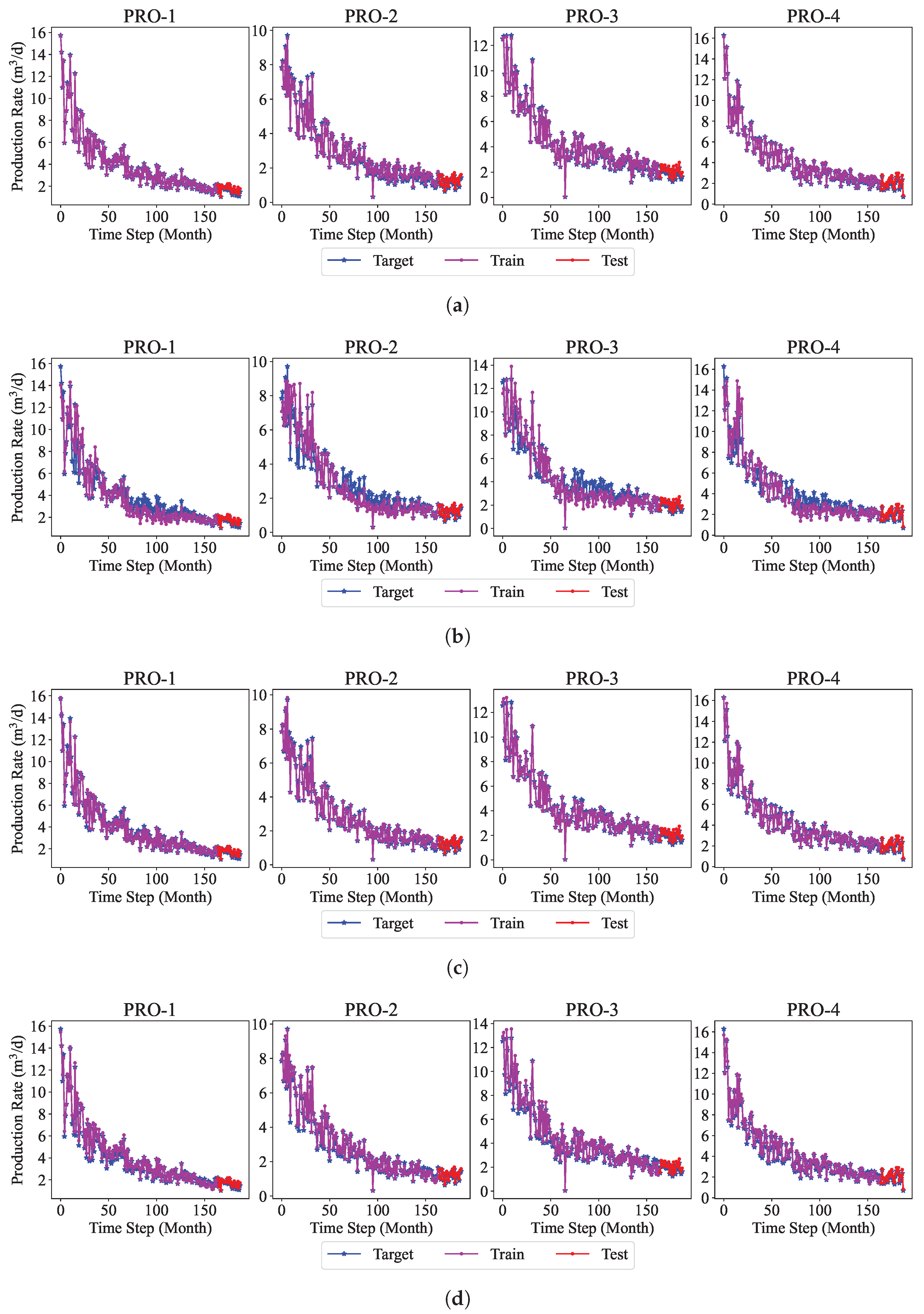
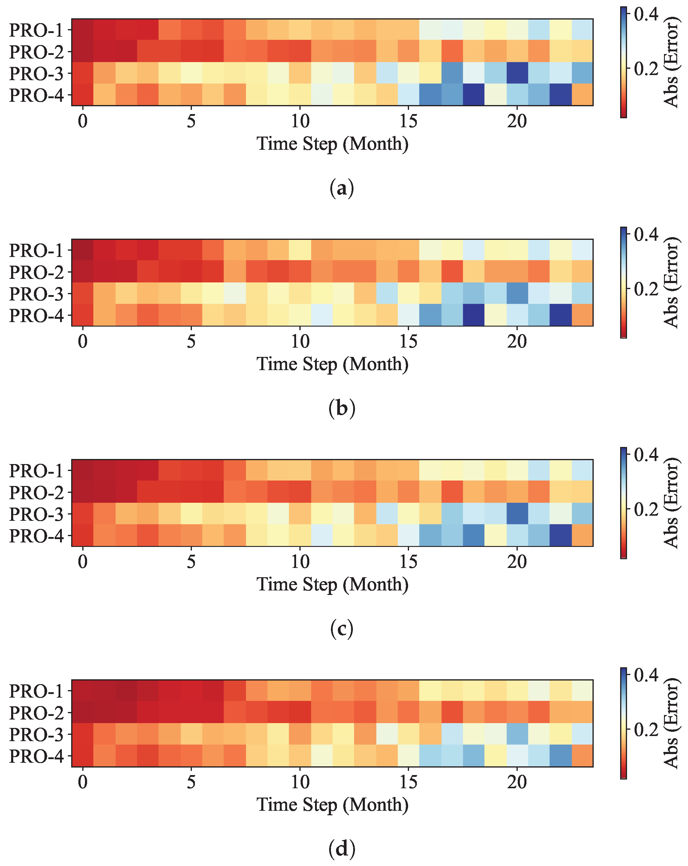
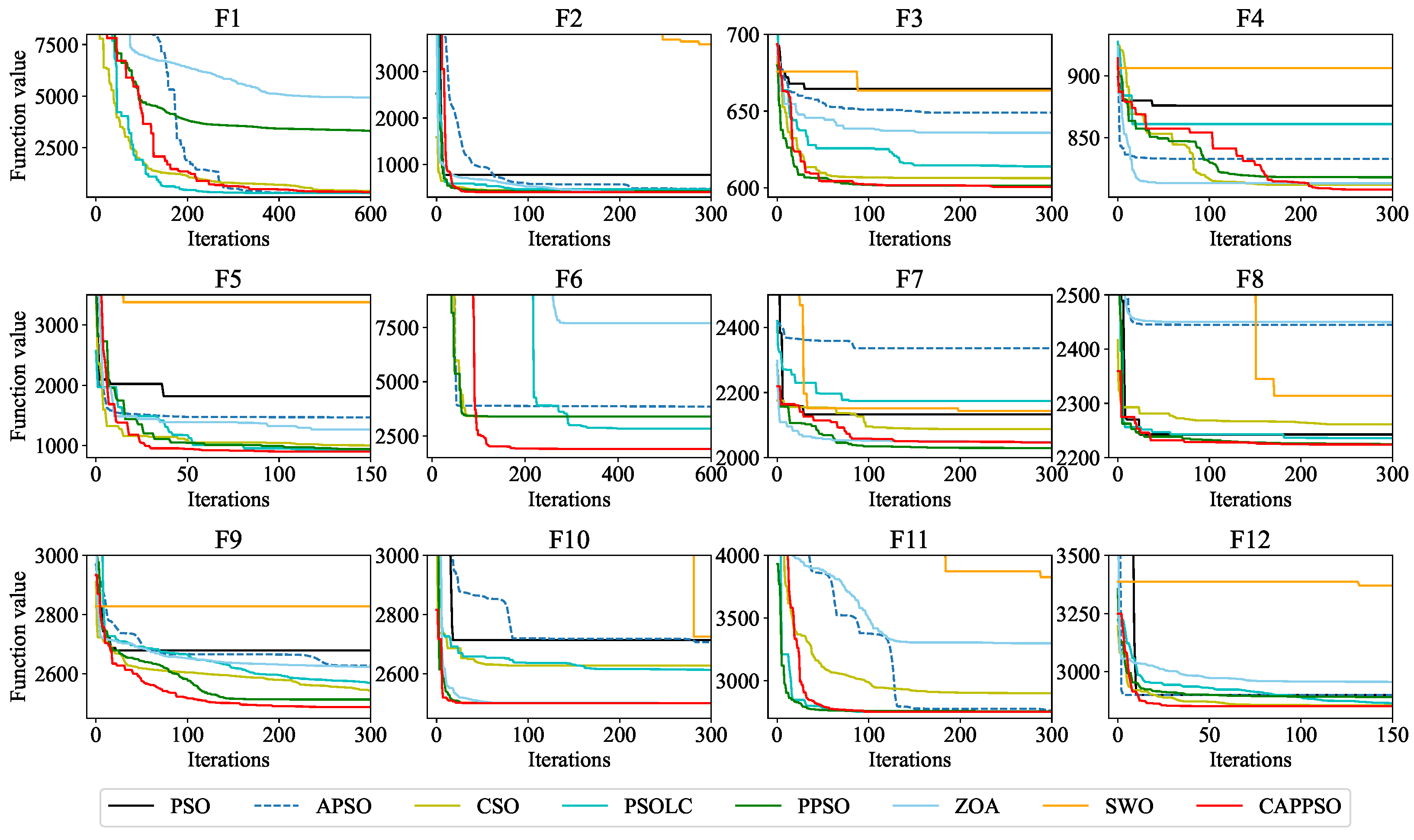
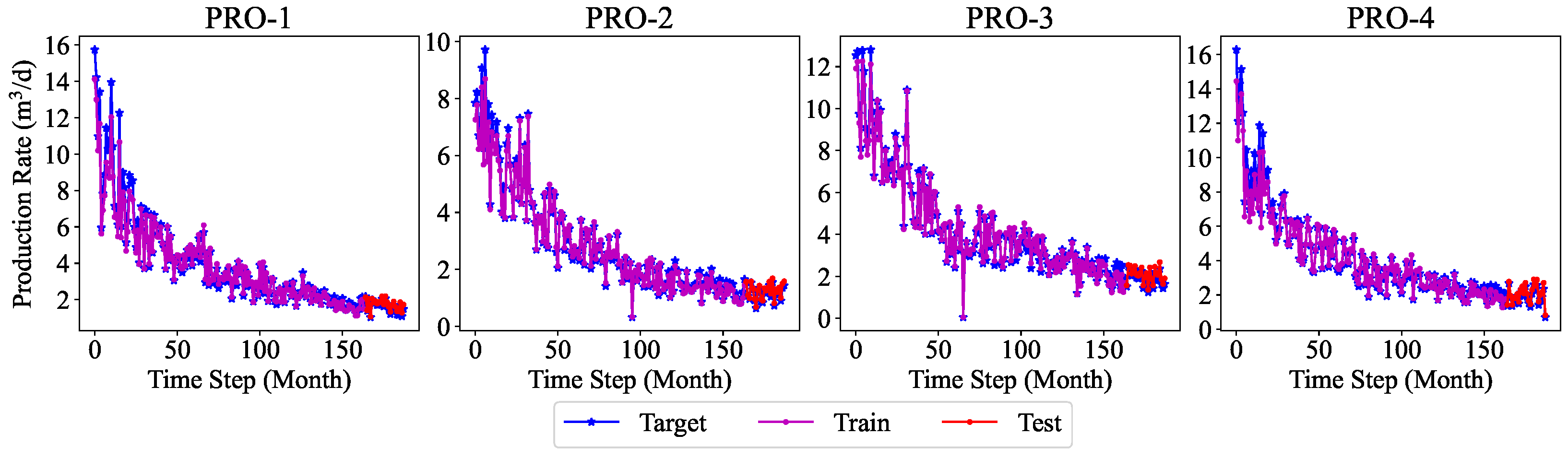
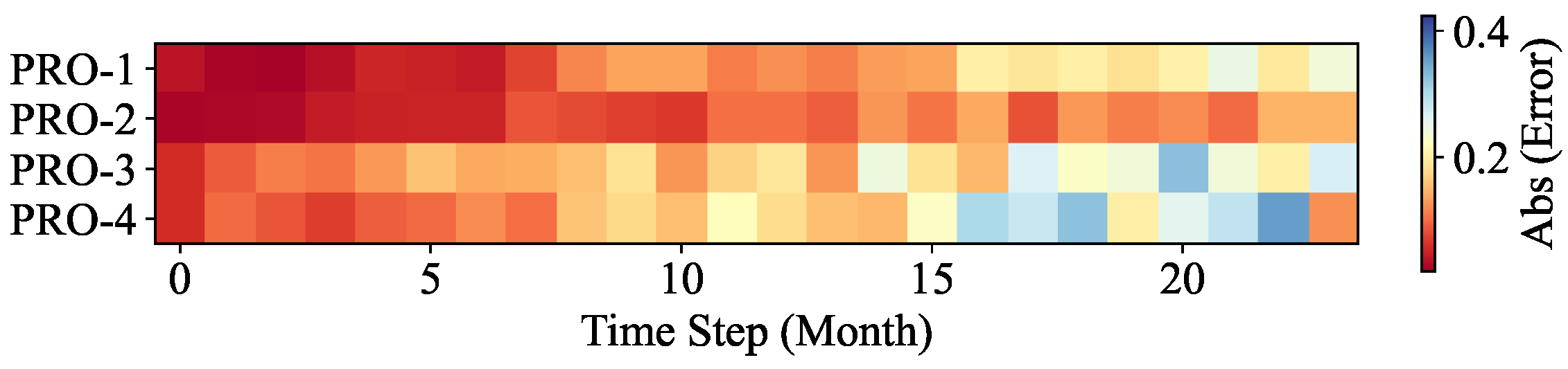
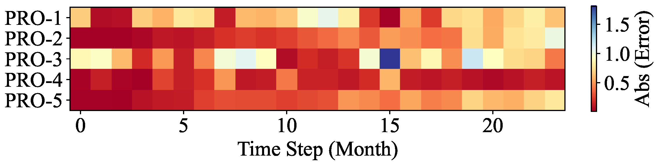
In this work, a machine learning model for multi-well production forecasting is implemented. This model incorporates physical information by introducing DCA, making it closely aligned with production practice. An improved PSO algorithm, CAPPSO, is proposed to adjust the importance proportions of each module derived from DCA within the loss function, thereby further improving the performance of the model. All the data required for model training can be obtained at the development site, making it practical. From the experimental results, the proposed model, i.e., LSTM-DCA and LSTM-DCA-CAPPSO, fits the experimental data better than the traditional BPNN, CNN, and LSTM models, leading the better performance in oil production forecasting. Furthermore, compared with traditional empirical parameters, a better combination of coefficients for DCA is found by CAPPSO, which reflects its engineering application value. The experimental results conducted on different reservoir types to validate the model’s generalization performance further demonstrate its high adaptability.

In the future, we plan to further improve the model so that it will have the same high forecasting capability in more types of oilfields by incorporating more physical mechanisms and dynamic adjustment strategies.

References

1. He, W.; Zhu, R.; Cui, B.; Zhang, S.; Meng, Q.; Bai, B.; Feng, Z.; Lei, Z.; Wu, S.; He, K.; et al. The geoscience frontier of Gulong shale oil: Revealing the role of continental shale from oil generation to production. Engineering 2023, 28, 79–92. [Google Scholar] [CrossRef]
2. Yuan, H.; Wang, Y.; Han, D.h. Evaluation of Pressure and Temperature Sensitivity of Heavy Oil Sands in North Sea through Laboratory Measurement and Rock-Physical Modeling. SPE J. 2023, 28, 1045–1061. [Google Scholar] [CrossRef]
3. Arps, J.J. Analysis of decline curves. Trans. AIME 1945, 160, 228–247. [Google Scholar] [CrossRef]
4. Mohammadmoradi, P.; Moradi, H.M.; Kantzas, A. Data-driven production forecasting of unconventional wells with apache spark. In Proceedings of the SPE Western Regional Meeting, Garden Grove, CA, USA, 2018; p. D041S011R006. [Google Scholar] [CrossRef]
5. Noshi, C.I.; Eissa, M.R.; Abdalla, R.M. An intelligent data driven approach for production prediction. In Proceedings of the Offshore Technology Conference, OTC, Houston, TX, USA, 6–9 May 2019; p. D041S048R007. [Google Scholar] [CrossRef]
6. Xiang, Y.; Zhuang, X.H. Application of ARIMA model in short-term prediction of international crude oil price. Adv. Mater. Res. 2013, 798, 979–982. [Google Scholar] [CrossRef]
7. Choi, T.M.; Yu, Y.; Au, K.F. A hybrid SARIMA wavelet transform method for sales forecasting. Decis. Support Syst. 2011, 51, 130–140. [Google Scholar] [CrossRef]
8. Pearson, K. The problem of the random walk. Nature 1905, 72, 342. [Google Scholar] [CrossRef]
9. Hou, A.; Suardi, S. A nonparametric GARCH model of crude oil price return volatility. Energy Econ. 2012, 34, 618–626. [Google Scholar] [CrossRef]
10. Zhang, J.L.; Zhang, Y.J.; Zhang, L. A novel hybrid method for crude oil price forecasting. Energy Econ. 2015, 49, 649–659. [Google Scholar] [CrossRef]
11. Mirmirani, S.; Cheng Li, H. A comparison of var and neural networks with genetic algorithm in forecasting price of oil. In Applications of Artificial Intelligence in Finance and Economics; Emerald Group Publishing Limited: Leeds, UK, 2004; Volume 19, pp. 203–223. [Google Scholar] [CrossRef]
12. Khashei, M.; Bijari, M. Fuzzy artificial neural network (p, d, q) model for incomplete financial time series forecasting. J. Intell. Fuzzy Syst. 2014, 26, 831–845. [Google Scholar] [CrossRef]
13. Yu, L.; Zhang, X.; Wang, S. Assessing potentiality of support vector machine method in crude oil price forecasting. EURASIA J. Math. Sci. Technol. Educ. 2017, 13, 7893–7904. [Google Scholar] [CrossRef] [PubMed]
14. Abo-Hammour, Z.; Abu Arqub, O.; Momani, S.; Shawagfeh, N. Optimization solution of Troesch’s and Bratu’s problems of ordinary type using novel continuous genetic algorithm. Discret. Dyn. Nat. Soc. 2014, 2014, 401696. [Google Scholar] [CrossRef]
15. Wang, J.; Wang, J. Forecasting energy market indices with recurrent neural networks: Case study of crude oil price fluctuations. Energy 2016, 102, 365–374. [Google Scholar] [CrossRef]
16. Chen, P.A.; Chang, L.C.; Chang, F.J. Reinforced recurrent neural networks for multi-step-ahead flood forecasts. J. Hydrol. 2013, 497, 71–79. [Google Scholar] [CrossRef]
17. Guo, T.; Xu, Z.; Yao, X.; Chen, H.; Aberer, K.; Funaya, K. Robust online time series prediction with recurrent neural networks. In Proceedings of the 2016 IEEE international conference on data science and advanced analytics (DSAA), Montreal, QC, USA, 17–19 October 2016; IEEE: Piscataway, NJ, USA, 2016; pp. 816–825. [Google Scholar] [CrossRef]
18. Hochreiter, S.; Schmidhuber, J. Long Short-Term Memory. Neural Comput. 1997, 9, 1735–1780. [Google Scholar] [CrossRef] [PubMed]
19. Lin, Y.; Yan, Y.; Xu, J.; Liao, Y.; Ma, F. Forecasting stock index price using the CEEMDAN-LSTM model. N. Am. J. Econ. Financ. 2021, 57, 101421. [Google Scholar] [CrossRef]
20. Jin, C.; Shi, Z.; Li, W.; Guo, Y. Bidirectional lstm-crf attention-based model for chinese word segmentation. arXiv 2021, arXiv:2105.09681. [Google Scholar] [CrossRef]
21. Droste, S.; Jansen, T.; Wegener, I. Upper and lower bounds for randomized search heuristics in black-box optimization. Theory Comput. Syst. 2006, 39, 525–544. [Google Scholar] [CrossRef]
22. Lu, W.; Cai, B.; Gu, R. Improved Particle Swarm Optimization Based on Gradient Descent Method. In Proceedings of the 4th International Conference on Computer Science and Application Engineering, Sanya, China, 20–22 October 2020. [Google Scholar] [CrossRef]
23. Salih, O.; Duffy, K.J. Optimization convolutional neural network for automatic skin lesion diagnosis using a genetic algorithm. Appl. Sci. 2023, 13, 3248. [Google Scholar] [CrossRef]
24. Zhang, X.; Jiang, Y.; Zhong, W. Prediction research on irregularly cavitied components volume based on gray correlation and pso-svm. Appl. Sci. 2023, 13, 1354. [Google Scholar] [CrossRef]
25. Kennedy, J.; Eberhart, R. Particle swarm optimization. In Proceedings of the ICNN’95-international conference on neural networks, IEEE, Perth, WA, Australia, 27 November–1 December 1995. [Google Scholar] [CrossRef]
26. Gou, J.; Lei, Y.X.; Guo, W.P.; Wang, C.; Cai, Y.Q.; Luo, W. A novel improved particle swarm optimization algorithm based on individual difference evolution. Appl. Soft Comput. 2017, 57, 468–481. [Google Scholar] [CrossRef]
27. Xia, X.; Gui, L.; Zhan, Z.H. A multi-swarm particle swarm optimization algorithm based on dynamical topology and purposeful detecting. Appl. Soft Comput. 2018, 67, 126–140. [Google Scholar] [CrossRef]
28. Sweilam, N.; Gobashy, M.; Hashem, T. Using particle swarm optimization with function stretching (SPSO) for inverting gravity data: A visibility study. Proc. Math. Phys. Soc. Egypt 2008, 86, 259–281. [Google Scholar]
29. Li, T.; Shi, J.; Deng, W.; Hu, Z. Pyramid particle swarm optimization with novel strategies of competition and cooperation. Appl. Soft Comput. 2022, 121, 108731. [Google Scholar] [CrossRef]
30. Kaur, G.; Arora, S. Chaotic whale optimization algorithm. J. Comput. Des. Eng. 2018, 5, 275–284. [Google Scholar] [CrossRef]
31. Raissi, M.; Perdikaris, P.; Karniadakis, G. Physics-informed neural networks: A deep learning framework for solving forward and inverse problems involving nonlinear partial differential equations. J. Comput. Phys. 2019, 378, 686–707. [Google Scholar] [CrossRef]
32. Misyris, G.S.; Venzke, A.; Chatzivasileiadis, S. Physics-informed neural networks for power systems. In Proceedings of the 2020 IEEE Power & Energy Society General Meeting (PESGM), Montreal, QC, USA, 2–6 August 2020; IEEE: Piscataway, NJ, USA, 2020; pp. 1–5. [Google Scholar] [CrossRef]
33. Kharazmi, E.; Zhang, Z.; Karniadakis, G.E. Variational physics-informed neural networks for solving partial differential equations. arXiv 2019. [Google Scholar] [CrossRef]
34. Yu, J.; Lu, L.; Meng, X.; Karniadakis, G.E. Gradient-enhanced physics-informed neural networks for forward and inverse PDE problems. Comput. Methods Appl. Mech. Eng. 2022, 393, 114823. [Google Scholar] [CrossRef]
35. Sharma, P.; Chung, W.T.; Akoush, B.; Ihme, M. A review of physics-informed machine learning in fluid mechanics. Energies 2023, 16, 2343. [Google Scholar] [CrossRef]
36. Wang, R.; Kashinath, K.; Mustafa, M.; Albert, A.; Yu, R. Towards physics-informed deep learning for turbulent flow prediction. In Proceedings of the 26th ACM SIGKDD International Conference on Knowledge Discovery & Data Mining, Virtual Event, 6–10 July 2020; pp. 1457–1466. [Google Scholar] [CrossRef]
37. Kong, W.; Dong, Z.Y.; Jia, Y.; Hill, D.J.; Xu, Y.; Zhang, Y. Short-Term Residential Load Forecasting Based on LSTM Recurrent Neural Network. IEEE Trans. Smart Grid 2019, 10, 841–851. [Google Scholar] [CrossRef]
38. Wang, N.; Zhang, D.; Chang, H.; Li, H. Deep learning of subsurface flow via theory-guided neural network. J. Hydrol. 2020, 584, 124700. [Google Scholar] [CrossRef]
39. Tang, H.Y.; He, G.; Ni, Y.Y.; Huo, D.; Zhao, Y.L.; Xue, L.; Zhang, L.H. Production decline curve analysis of shale oil wells: A case study of Bakken, Eagle Ford and Permian. Pet. Sci. 2024, 21, 4262–4277. [Google Scholar] [CrossRef]
40. Zang, J.; Wang, J.; Zhang, K.; El-Alfy, E.S.M.; Mańdziuk, J. Expertise-informed Bayesian convolutional neural network for oil production forecasting. Geoenergy Sci. Eng. 2024, 240, 213061. [Google Scholar] [CrossRef]
41. Chen, Z.; Wang, C.; Luo, H.; Wang, H.; Chen, Y.; Wen, C.; Yu, Y.; Cao, L.; Li, J. Vehicle Detection in High-Resolution Aerial Images Based on Fast Sparse Representation Classification and Multiorder Feature. IEEE Trans. Intell. Transp. Syst. 2016, 17, 2296–2309. [Google Scholar] [CrossRef]
42. Li, C. Principles of Reservoir Engineering; Petroleum Industry Press: Beijing, China, 2005. [Google Scholar]
43. Tavazoei, M.S.; Haeri, M. Comparison of different one-dimensional maps as chaotic search pattern in chaos optimization algorithms. Appl. Math. Comput. 2007, 187, 1076–1085. [Google Scholar] [CrossRef]
44. Feng, J.; Zhang, J.; Zhu, X.; Lian, W. A novel chaos optimization algorithm. Multimed. Tools Appl. 2017, 76, 17405–17436. [Google Scholar] [CrossRef]
45. Jansen, J.D.; Fonseca, R.M.; Kahrobaei, S.; Siraj, M.; Van Essen, G.; Van den Hof, P. The egg model–A geological ensemble for reservoir simulation. Geosci. Data J. 2014, 1, 192–195. [Google Scholar] [CrossRef]
46. Wang, N.; Liao, Q.; Chang, H.; Zhang, D. Deep-learning-based upscaling method for geologic models via theory-guided convolutional neural network. Comput. Geosci. 2023, 27, 913–938. [Google Scholar] [CrossRef]
47. Kumar, A.; Price, K.V.; Mohamed, A.W.; Hadi, A.A.; Suganthan, P.N. Problem Definitions and Evaluation Criteria for the Cec 2022 Special Session and Competition on Single Objective Bound Constrained Numerical Optimization; Technical Report; Nanyang Technological University: Singapore, 2021. [Google Scholar]
48. Zhan, Z.H.; Zhang, J.; Li, Y.; Chung, H.S.H. Adaptive particle swarm optimization. IEEE Trans. Syst. Man, Cybern. Part B (Cybern.) 2009, 39, 1362–1381. [Google Scholar] [CrossRef] [PubMed]
49. Van den Bergh, F.; Engelbrecht, A.P. A cooperative approach to particle swarm optimization. IEEE Trans. Evol. Comput. 2004, 8, 225–239. [Google Scholar] [CrossRef]
50. Molaei, S.; Moazen, H.; Najjar-Ghabel, S.; Farzinvash, L. Particle swarm optimization with an enhanced learning strategy and crossover operator. Knowl.-Based Syst. 2021, 215, 106768. [Google Scholar] [CrossRef]
51. Trojovská, E.; Dehghani, M.; Trojovskỳ, P. Zebra optimization algorithm: A new bio-inspired optimization algorithm for solving optimization algorithm. IEEE Access 2022, 10, 49445–49473. [Google Scholar] [CrossRef]
52. Abdel-Basset, M.; Mohamed, R.; Jameel, M.; Abouhawwash, M. Spider wasp optimizer: A novel meta-heuristic optimization algorithm. Artif. Intell. Rev. 2023, 56, 11675–11738. [Google Scholar] [CrossRef]
53. Peters, E.; Arts, R.J.; Brouwer, G.K.; Geel, C.R.; Cullick, S.; Lorentzen, R.J.; Chen, Y.; Dunlop, K.N.B.; Vossepoel, F.C.; Xu, R.; et al. Results of the Brugge Benchmark Study for Flooding Optimization and History Matching. SPE Reserv. Eval. Eng. 2010, 13, 391–405. [Google Scholar] [CrossRef]
54. Hsieh, D.A. A heteroscedasticity-consistent covariance matrix estimator for time series regressions. J. Econom. 1983, 22, 281–290. [Google Scholar] [CrossRef]
55. Kotz, S.; Johnson, N.L. (Eds.) The Probable Error of a Mean. In Breakthroughs in Statistics: Methodology and Distribution; Springer: New York, NY, USA, 1992; pp. 33–57. [Google Scholar] [CrossRef]
Figure 1. Oilfield development mode, where I, II and III represent production increase, production stability and production decline, respectively.
Eng 06 00172 g001
Figure 2. Schematic illustration of the memory cell structure in LSTM and the direction of information flow regulated by gating mechanisms.
Eng 06 00172 g002
Figure 3. In pyramid building, the topmost apex serves as the first layer, with the layer index i increasing in ascending order from the top to the bottom of the pyramid.
Eng 06 00172 g003
Figure 4. The sliding window of length 3 ( s = 3 ) generates samples step by step [40].
Eng 06 00172 g004
Figure 5. Model structure of LSTM-DCA, including the data processing and flow process, as well as the hybrid of the loss function during training.
Eng 06 00172 g005
Figure 6. Reservoir model displaying the position of the injectors (blue) and producers (red).
Eng 06 00172 g006
Figure 7. The oil production forecasting results of (a) BPNN, (b) CNN, (c) LSTM, and (d) LSTM-DCA on the training set (purple) and testing set (red), including target values (blue). The Y-axis label content of each row of figures is the text on the far left.
Eng 06 00172 g007
Figure 8. The forecasting error results of (a) BPNN, (b) CNN, (c) LSTM, and (d) LSTM-DCA on the testing set.
Eng 06 00172 g008
Figure 9. Convergence situation of functions F1-F12 of CEC2022 with d = 10 .
Eng 06 00172 g009
Figure 10. The oil production forecasting results of LSTM-DCA-CAPPSO on the training set (purple) and testing set (red), including target values (blue). The Y-axis label content of figures is the text on the far left.
Eng 06 00172 g010
Figure 11. The forecasting error results of LSTM-DCA-CAPPSO on the testing set.
Eng 06 00172 g011
Figure 12. The geographical location of the Brugge reservoir prototype is roughly circled in red.
Eng 06 00172 g012
Figure 13. Brugge reservoir with 5 injecting wells (I1, …, I5) and 5 producing wells (P1, …, P5).
Eng 06 00172 g013
Figure 14. The oil production forecasting results of LSTM-DCA-CAPPSO on the testing set (red), including target values (blue) for the Brugge reservoir. The Y-axis label content of figures is the text on the far left.
Eng 06 00172 g014
Figure 15. The forecasting error results of LSTM-DCA-CAPPSO on the testing set for the Brugge reservoir.
Eng 06 00172 g015