Reliability Analysis and Parameter Selection for IoT Communication Based on Deep Learning

Abstract

This article first constructs a multi-layer deep learning neural network to help understand the structural characteristics of communication data, thereby learning complex functions and obtaining the predicted network values. At the same time, signal transmission is achieved through the interconnection of neurons, the representation performance of which is enhanced through activation functions; this completes the modeling of IoT communication models. Then, we use the analytic hierarchy process to construct a deep learning autoencoder and extract the feature elements of network communication reliability parameters. Finally, we use the obtained total reliability indicators as features for automatic coding and evaluate the mapping relationship between indicators. The results show that the success rates of handovers in deep leaning-based IoT communication based are all greater than 99.6%. The predicted transmission rate can reach a maximum of 99.5%, achieving error free communication output and improving fidelity.

1. Introduction

With the rapid advancement of technology, the Internet of Things (IoT) continues to expand in both scale and complexity, resulting in increasingly sparse and heterogeneous communication links. As a cornerstone of the overall IoT infrastructure, wireless communication reception plays a critical role in ensuring reliable information exchange [1,2]. As digitalization deepens across society, users’ reliance on internet-based services grows due to their convenience, speed, and quality. However, this increased dependency also raises concerns about data security and privacy. Malicious entities often employ techniques such as packet tracing and traffic analysis to infer sender and receiver identities, thereby compromising sensitive information [3,4]. Thus far, many large and complex devices have been developed by humans. The common feature of these systems is their complex structure and powerful functionality. The predetermined functions require complex hardware and software support for completion and sometimes human participation. System malfunctions cause losses to varying degrees and in various aspects [5,6]. Therefore, research on the reliability of IoT communication has significant theoretical significance and practical value.

This article aims to improve the efficiency and reliability of Internet of Things (IoT) communication networks by leveraging deep learning techniques. The primary objective is to construct a robust IoT communication model that can effectively handle complex network environments and optimize communication performance. The main contribution of this study lies in integrating neural network mechanisms into the communication modeling process, introducing a novel approach that combines feature abstraction, nonlinear enhancement, and dimensional reduction for communication parameters. The novelty of this work lies in the fusion of autoencoder-based feature extraction with AHP-based dimensional reduction within an IoT-specific neural architecture, offering a new perspective on communication modeling under intelligent frameworks. The rest of this paper is organized as follows: Section 2 reviews related work; Section 3 describes the proposed methodology in detail; Section 4 presents experimental validation and results; Section 5 discusses the findings; and Section 6 concludes the paper with insights and future directions.

2. Literature Review

Roseela, J and others used microcontrollers to achieve underwater wireless communication design. By deploying various unmanned motors or units underwater and utilizing the data switching ability, they provided higher bandwidth functions than typical systems, greatly reducing energy consumption and solving the technical problem of short-distance Wi Fi connection [7]. Dong, N designed a malicious intrusion detection model for cloud data center network communication. Firstly, data preprocessing includes three parts: normal sample data modeling, standard data membership calculation, and anomaly determination. Then, the feature value collection phase is completed, before finally, intrusion detection classification and trust value calculation are achieved, and malicious intrusion detection for cloud data center network communication obtained. This method improves the intrusion detection rate, reducing the detection time and false alarm rate [8]. Agrawal, N utilizes the OSI LAYER model to achieve network information transmission, which is a complete framework that provides all the information about its work and the connections between them. This method not only transmits information but also transmits it in a secure manner, which helps us understand network characteristics [9]. Mahler, T proposed a multi-input multi-output wireless channel measurement system that utilizes multiple software-defined radio platforms on both the transmitter and receiver. This method was validated through ray tracing channel simulation. Antenna synthesis methods are applied to mobile single-channel and mobile multi-channel receivers, before the synthetic antenna system, based on the antenna radiation pattern and corresponding channel capacity, is valuated [10].

Deepa, A proposes a new high-speed VLSI architecture for encoding Reed Solomon codes, with pipelining and parallelization enabling high-speed input transmission with minimal latency. By introducing new modifications to the LFSR, they modify to an infinite pulse response filter, which eliminates the speed bottleneck of the basic Reed Solomon encoder based on LFSR and improves the communication application data rate [11]. Samyuel, N. B, and others propose secure network architecture based on recursive networks to address most of the network defects in existing network protocols. successfully prevents network flow attack threats, especially in closed environments such as local area networks [12]. Suma, V adopts a scalable distributed computing framework and analyzes resource allocation requirements and shared parameters through cyclic learning, thereby improving end user communication reliability. With the assistance of UCS and estimated resource requirements, sensor end users of WIoT can achieve higher communication rates [13]. Babu, C discusses a power monitoring and control system composed of inverters, measuring instruments, solar charging controllers, relays, and other main components in a medium voltage smart grid. This indicates that the Internet of Things plays a crucial role in communication between sensors and power systems. Through bidirectional network communication media such as the Internet of Things, power system supply reliability has been improved [14]. Moriyama, M improved the physical layer communication of the downlink using spatial diversity. By combining spatial block coding and cyclic delay diversity, communication stability is effectively improved by appropriately setting the cyclic offset [15].

Liaskos, C et al. utilized software to define the basic principles of metasurfaces, applying them to existing network mask systems. Firstly, they introduced SDM’s integrated architecture and corresponding complex underlying physical characteristics. Then, software abstraction—which can achieve precise, software-defined signal propagation and wireless channel customization [16]—was proposed to enable surfaces to interact in a physically independent manner. Kanno, S et al. used under-sampling to measure radio signals in the high-frequency band using low sampling frequencies, converting them into low-frequency image signals. The instrument for measuring high-frequency radio signals is lower cost with higher communication resolution, and the simulation results of real-time sampling are very consistent with those of under-sampling [17]. Gao, L. et al. constructed an indicator system based on the characteristics and applications of wireless communication systems from three aspects: basic communication capability, communication reliability, and interconnection capability. Then, they used the ADC method to evaluate the effectiveness of wireless communication and provide recommendations for system development [18].

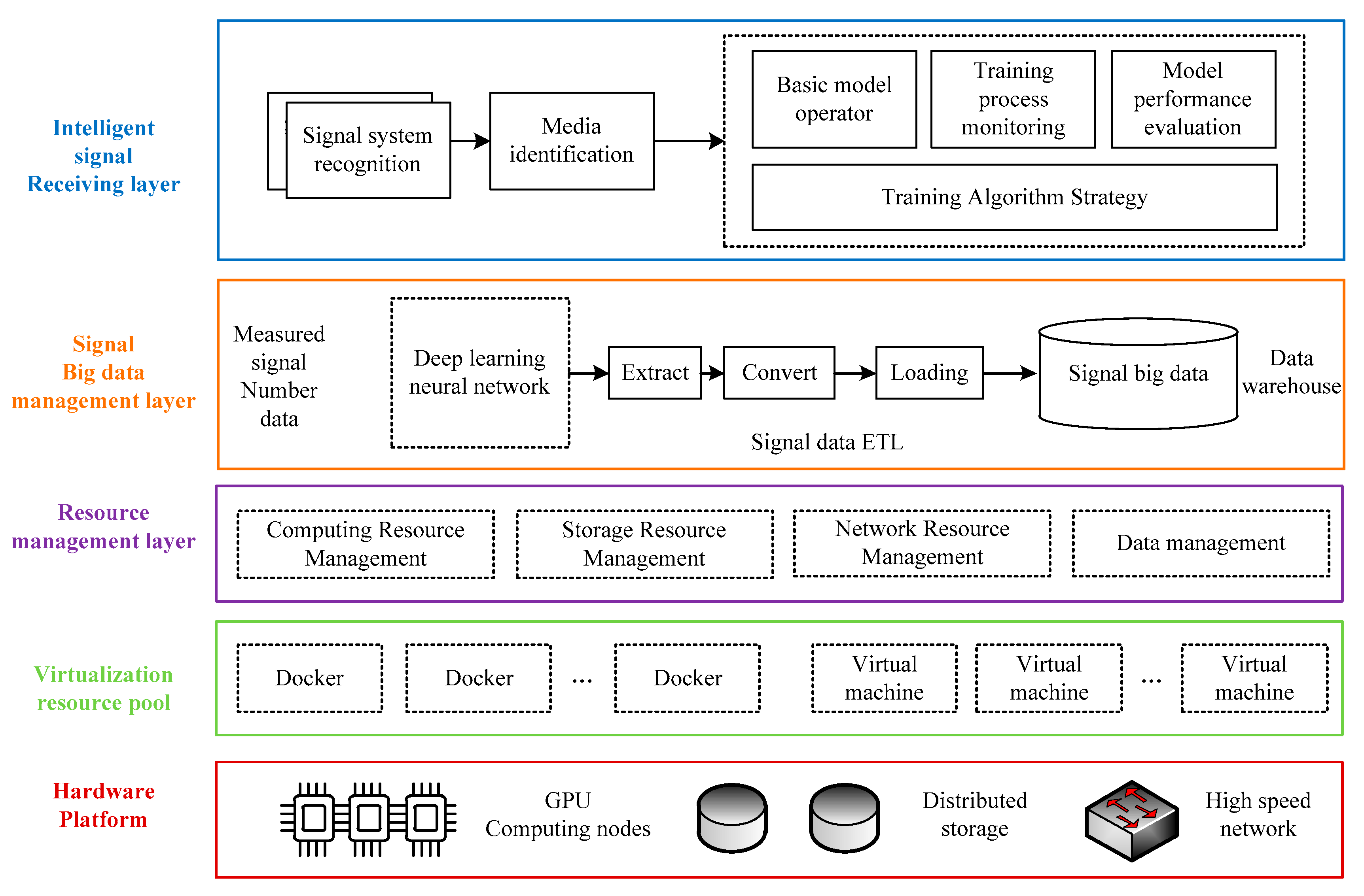
3. Building an Internet Communication Model Based on Deep Learning

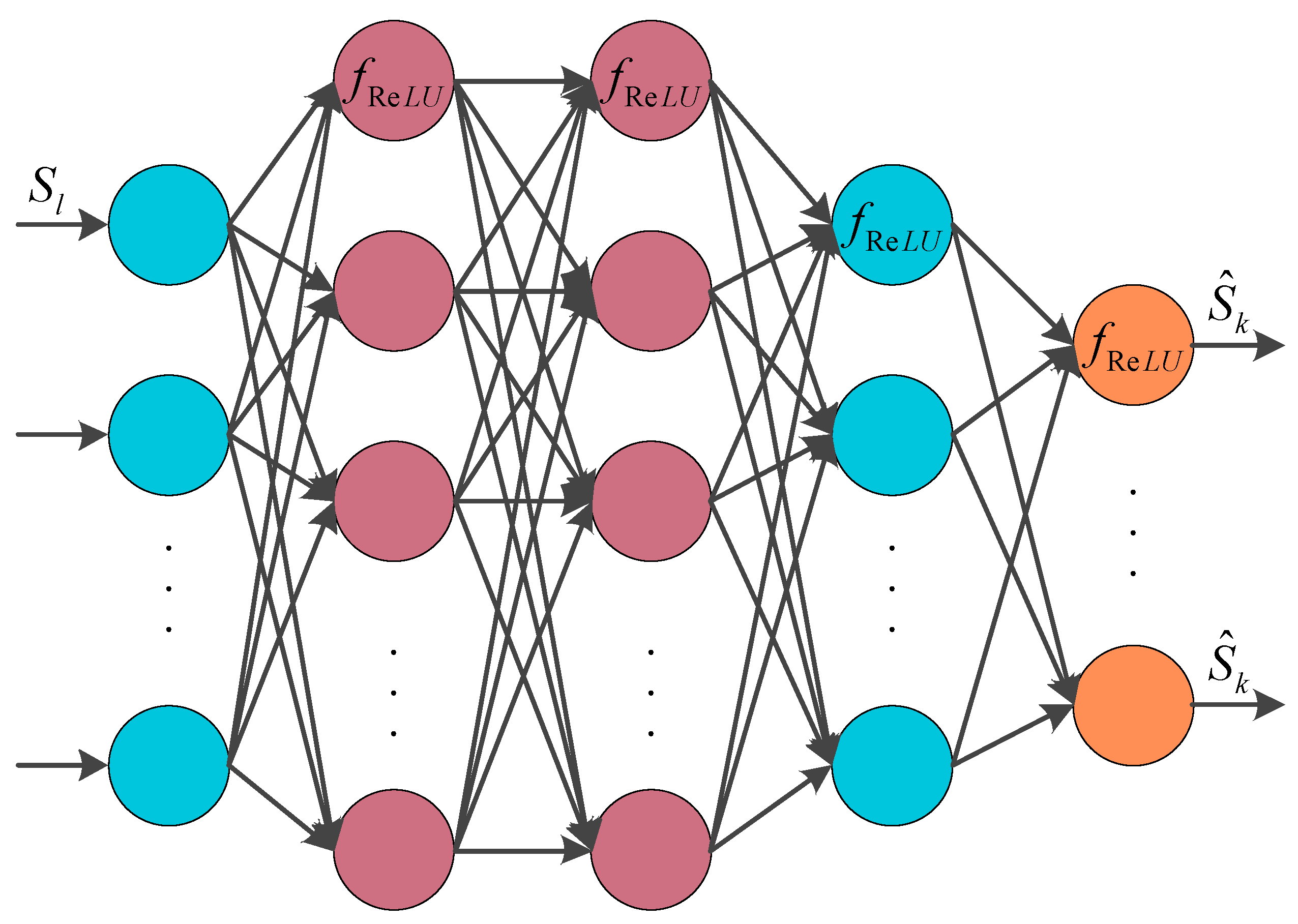
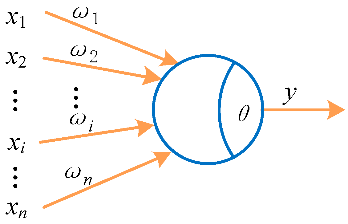
3.1. Deep Learning Network

Originally derived from the study of artificial neural networks, deep technology is a separate discipline from machine learning. It consists of three key structures: neural, deep belief and self-coding networks. Deep learning is used to build multi-layer artificial neural networks to obtain powerful structural features such as extraction, pattern recognition and complex nonlinear functions [19,20,21].

Deep neural networks include at least one hidden layer. In multi-layer output neural networks, initial features are converted into output expressions of high-level features using layer-by-layer processing techniques by means of abstraction and extraction. The communication model is constructed by learning complex functions [22,23]. The structure of the network is shown in Figure 1; the forward propagation process of the neural network is such that the original data are introduced into the input layer and, after passing layer-by-layer, the predicted value of the network is finally obtained in the output layer. This layer-by-layer abstraction and information transfer process enables the deep neural network to capture the complex features of the input data for more effective learning and prediction. This study uses the ReLU (rectified linear unit) activation function in the hidden layer, mainly because of its high computational efficiency, stable gradient propagation, and good performance in processing high-dimensional sparse data. In addition, in order to perform probability output of multi-classification tasks, the output layer of the model still uses the Softmax function to ensure that the results are interpretable and normalized.

Assuming that the input layer of the deep learning network is $v$ and the hidden layer is $h$, the layers are opposite and all connected to each other. The energy function and probability distribution function are, respectively, represented as follows:

$$E(v,h,\theta )=-a^{\mathrm{T}}v-b^{\mathrm{T}}h-v^{\mathrm{T}}Wh=-{\displaystyle \sum _{i\in v}{a}_i}{v}_i-{\displaystyle \sum _{i\in h}{b}_i}{h}_i-{\displaystyle \sum _{i,j}{v}_i}{h}_i{\omega }_{ij},$$

(1)

$$p(v,h,\theta )={\displaystyle \frac{1}{Z}}{e}^{-E(v,h,\theta )}.$$

(2)

Among them, $v_i$ represents the input layer node state, $h_i$ represents the hidden layer node state, and $a_i$  $b_i$ represent the corresponding layer node offset. ${\omega }_{i,j}$ is the connection weight, $\theta =\{W,a,b\}$ is the parameter optimization weight, and $Z$ is the normalization coefficient, namely

$$Z={\displaystyle \sum _{v,h}{e}^{-E(v,h,\theta )}}.$$

(3)

Based on fitting input data, this article utilizes the maximum likelihood learning method for maximization. During the training process, if it is necessary to reconstruct the parameter weights of the deep learning network, the full-time update method is as follows:

$$\left\{\begin{array}{l}\mathrm{\Delta }{\omega }_{ij}=\epsilon *\left({〈v_i{h}_i〉}_{\mathrm{data}}-{〈v_i{h}_i〉}_{\mathrm{recon}}\right)\hfill \\ \mathrm{\Delta }{\alpha }_i=\epsilon *\left({〈v_i〉}_{\mathrm{data}}-{〈v_i〉}_{\mathrm{recon}}\right)\hfill \\ \mathrm{\Delta }{b}_i=\epsilon *\left({〈h_i〉}_{\mathrm{data}}-{〈h_i〉}_{\mathrm{recon}}\right).\hfill \end{array}\right.$$

(4)

After pre-training, the communication model obtains an initial weight value, which requires fine-tuning for optimization. The adjusted objective function is as follows:

$$f(\theta )=-{\displaystyle \sum _i{y}_i^{\mathrm{T}}}\lg y_i^{\prime }.$$

(5)

In the formula, $\theta =\left\{{\omega }_1,{\omega }_2,{\omega }_3,{\omega }_4,{\omega }_5,\omega \right\}$ is the fine-tuning network parameter, $y_i$ is the sample label, and ${y_i}^{\prime }$ is the prediction result.

$$\widehat{s}=f_{\mathrm{Re}LU}^{(out)}\left(f_{\mathrm{Re}LU}^{(3)}\left(f_{\mathrm{Re}LU}^{(2)}\left(f_{\mathrm{Re}LU}^{(1)}\left(s{\omega }^{(1)}+b^{(1)}\right){\omega }^{(2)}+b^{(2)}\right){\omega }^{(3)}+b^{(3)}\right){\omega }^{(out)}+b^{(out)}\right)$$

(6)

In Equation (6), ${\omega }_{ij}^{(l)}$ Represents the connection weight between the $i$-th neuron node in layer $l-1$ and the $j$-th neuron node in layer $l$, and $b_j^{(l)}$ represents the offset of the $j$-th neuron node in layer $l$.

3.2. Extracting Signal Features

Neurons are the basic building blocks of deep learning networks. In biological neural networks, neurons have a complex structure of multiple inputs, single outputs, and interconnections. When the potential of a neuron exceeds a threshold, it is activated and transmits chemicals to other neurons [24,25]. Figure 2 shows the neuron structure, where ${\omega }_i$ represents the corresponding $x_i$ weight. $n$ is the input is signal from other neurons and $x_i$ is the communication data into the $i$th neuron, with ${\omega }_i$ representing the corresponding weights.

The neuron first multiplies each input signal by its corresponding weight and sums the result, which is the weighted total input. Afterwards, the difference between the input value and the neuron threshold $\theta$ is fed into the activation function to obtain the neuron output value of $y$. The entire process can be expressed as follows:

$$y=f\left({\displaystyle \sum _{i=1}^n{\omega }_i}{x}_i-\theta \right).$$

(7)

The activation function is an important component of neural networks. Without it, neurons can only perform linear mapping on the input and output, resulting in the latter being only a linear transformation relative to the former, and the approximation effect is poor for complex objective functions. The activation function enhances the representation performance of neurons through nonlinear mapping, thereby enhancing the network’s complex function fitting ability. The initial activation function used was the step function:

$$f_{\mathrm{sgn}}(x)=\left\{\begin{array}{ll}1,\hfill & x\ge 0\hfill \\ 0,\hfill & x<0.\hfill \end{array}\right.$$

(8)

The step function maps the input values to 0 and 1 to simulate the excitation and inhibition neuron states, so neural networks often use continuous nonlinear activation functions, namely

$$f_{\mathrm{Re}LU}(x)=\max (0,x).$$

(9)

3.3. IoT Communication Model

The communication system is an information system established utilizing the basic laws of nature and human sensory accessibility [26]. Improved communication methods and technologies are the driving force for human exploration. Deep neural networks are applied to IoT communication systems, where intelligent processing and learning technologies are effective methods of enhancing communication technology dissemination [27,28]. Therefore, this article draws on the functions of automatic feature extraction and autonomous learning in deep learning methods to establish a deep learning network [29,30]. Interference noise is perceived through neurons’ recognition of radio frequency signals, and the channel capability is restored at the information receiving end.

Figure 3 shows the basic structure of the internet communication model, which centers on the signal data management layer and utilizes deep learning networks to depict and describe wireless channels from multiple feature dimensions. Data storage can be achieved by extracting, converting, and loading signal data, and resource management tools such as virtual machines are used to achieve fast elastic load balancing for communication signal resources and the ability to perceive global features. Additional tools in this regard are deep learning, autonomously adjusting model-related parameters and performance evaluation, and continuously improving the model’s communication reliability and fault recovery ability.

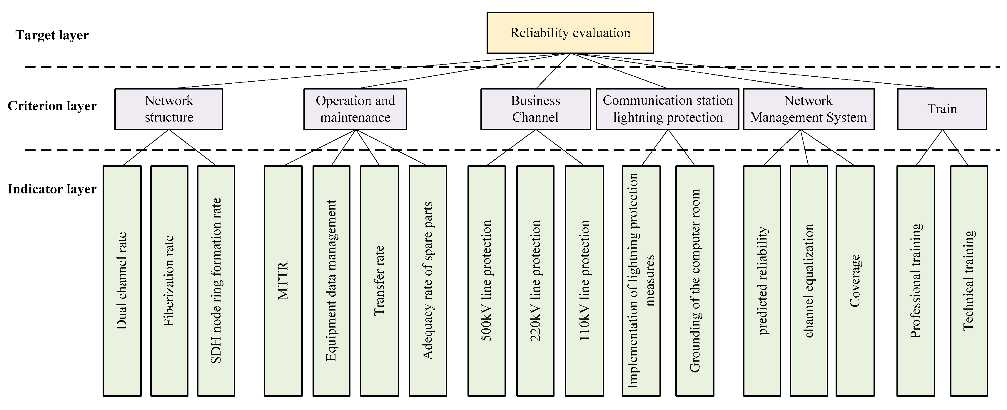
4. Selection of Communication Model Reliability Parameters

4.1. Establishment of Parameter System

Reliability parameters refer to the probability that IoT communication meets its business indicators and can be used as a reliability indicator for evaluating communication. Figure 4 shows the communication reliability parameter architecture.

This article utilizes the analytic hierarchy process (AHP) to construct a deep learning-based autoencoder that extracts network communication parameters from advanced feature data. AHP is chosen due to its clear hierarchical structuring of complex decision problems, ability to incorporate both qualitative and quantitative criteria, and its well-established consistency checking mechanism, which ensures reliable weighting of features. Compared to other multi-criteria decision analysis (MCDA) methods such as TOPSIS or fuzzy AHP, AHP offers more intuitive pairwise comparisons and easier interpretability, making it more suitable for guiding the design and parameter selection in the autoencoder training process. Furthermore, the method facilitates integrating expert judgment with data-driven insights, enhancing the model’s robustness and applicability.

An IoT communication dataset, which can be described as $X=\left\{x_1,x_2,\dots ,x_m\right\}$, is carefully processed to produce accurate outputs and build a complete dataset $Y=\{y_1,y_2,\dots ,y_n\}$. Assuming the set of related transformation parameters is $Q=(q,t)$, $x$ is transformed into $\mathrm{Z}$ through the mapping relationship of hidden layer $y$. The calculation formula can be expressed as follows:

$$A(x)=\alpha *(qx+t).$$

(10)

Among them, $A(x)$ is the mapping relationship of the hidden layer, $a$ is the weighting factor parameter, $q$ is the weight parameter matrix after dimensionality reduction, and $t$ is the offset vector parameter. In the encoder, in order to maintain the error value between the input and output vectors within a controllable range, the discrete structure of the loss function $K$ is used for calculation, namely

$$K(x,z)={\displaystyle \sum _{i=1}^n{x}_i}\log z_i.$$

(11)

In the above equation, examining the number of data samples input by $n$, $z_i$ is the parameter value of the $i$-th sample in hidden layer $z$, and $x_i$ is the parameter value of the $i$-th vector in the input vector set.

Assuming the input training sample is $x$ during the training process, the average parameter $\partial$ is calculated by adding the corresponding penalty weight parameter value $\beta$ and the calculation process is represented as follows:

$$\partial ={\displaystyle \sum _{i=1}^n{\beta }^{*}}{x}_i{\displaystyle \frac{1}{n}}.$$

(12)

Assuming that the communication parameter range of the Internet of Things is $\mu$ and satisfies $0\le \mu \le 1$, the communication data are in a more dangerous state as the $\mu$ value approaches 1. On the contrary, if the value of $\mu$ is closer to 0, it is safer. Therefore, for this parameter $\mu$, its calculation formula is as follows:

$$\mu =\epsilon *d+P*(1-\epsilon ).$$

(13)

In the formula, $\epsilon$ is the empirical factor parameter that satisfies $0\le \epsilon \le 1$, $d$ is the subjective weight parameter for the feature, and $p$ is the objective feature weight parameter.

4.2. Indicator Evaluation

In order to further evaluate the reliability of the IoT communication model, the reliability index is set as $X=\left\{x_1,x_2,\dots ,x_n\right\}$, the reliability evaluation criterion is $Z=\left\{{\tau }_1,{\tau }_2,\dots ,{\tau }_n\right\}$, and the final reliability measure is $y$, $y=f\left(g\left(x_1,x_2,\dots ,x_n\right)\right)$. $g(\cdot )$$f(\cdot )$ represent the mapping relationship from reliability indicators to reliability criteria, and that from reliability criteria to reliability metrics, respectively. The traditional reliability modeling method based on analytic hierarchy process usually the $g(\cdot )$ and $f(\cdot )$ models as linear mappings.

For network structure reliability evaluation criteria, there are three reliability indicators $\left\{x_1,x_2,x_3\right\}$. The traditional analytic hierarchy process uses a pairwise comparison method to establish a comparison matrix and quantify the mapping between $g(\cdot )$ and $f(\cdot )$, namely

$$g(\cdot )\to {\tau }_1=\left(\begin{array}{ccc}{u}_{1,1}& \dots & u_{1,3}\\ ⋮& u_{i,j}& ⋮\\ u_{3,1}& \dots & u_{3,3}\end{array}\right)\left(\begin{array}{c}{x}_1\\ ⋮\\ x_3\end{array}\right)$$

(14)

$$f(\cdot )\to y=\left(\begin{array}{ccc}{v}_{1,1}& \dots & v_{1,6}\\ ⋮& v_{i,j}& ⋮\\ v_{6,1}& \dots & v_{6,6}\end{array}\right)\left(\begin{array}{c}{\tau }_1\\ ⋮\\ {\tau }_6\end{array}\right)$$

(15)

In the formula, $u_{i,j}$ represents the importance of reliability index $i$ to reliability index $j$, and $u_{i,j}=1/u_{j,i},v_{i,j}$ represents the importance of reliability criterion $i$ to reliability criterion $j$.

The input vector of the auto-coded features is the hierarchized indicator $\overrightarrow{x}=\left\{x_1,x_2,\dots ,x_n\right\}$. The parameter $(w,b)$ is obtained by optimization and the input vector $\overrightarrow{y}=\left\{y_1,y_2,\dots ,y_n\right\}$ is reconstructed into $\overrightarrow{y}$. Based on the above, the reliability index is effectively encoded and reconstructed, thereby improving the accuracy of the model’s reliability assessment in complex communication environments.

5. Reliability Analysis of IoT Communication Model

5.1. Parameter System

During the data collection process, the design of the system operating environment is often overlooked, especially when communication power supply parameters may conflict. To avoid parameter conflicts during operation, this study integrates an IoT communication model to identify and monitor key parameters within the system’s operating environment.

The experiment selected the JM-5A communication power supply as the research object. This power supply can generate various vibration signals and allows adjustment of the vibration amplitude through a potentiometer. The experiment was conducted in a local area network environment, using a photo box device to test system performance and meet the requirements for parameter identification.

This is a real-world experiment, where both valid and invalid data were used to execute all functional use cases within the model, evaluating the communication model’s performance and parameter identification accuracy. To compare results clearly, an IoT-based communication model was designed as the experimental group, while a traditional distributed communication system was used as the control group. The parameter identification accuracy of the two methods under different standard voltages was compared, improving the credibility of the data collection.

A comparison of parameter identification accuracy is shown in

Table 1. Comparison results of parameter recognition accuracy.

Standard Voltage	Experimental Group	Relative Error	Control Subjects	Relative Error
3.0	3.026	0.025%	4.028	3.528%
2.0	1.924	0.022%	3.252	1.248%
1.0	0.983	0.016%	4.032	1.625%
−1.0	−1.025	0.034%	3.059	2.318%
−2.0	−2.038	0.041%	3.648	3.058%
−3.0	−2.989	0.023%	5.628	4.629%

. Under different standard voltages, the communication model based on the Internet of Things in this article is closer to the actual values in parameter identification, with an error of only about 0.035%. By integrating IoT technology, the system can fully perceive changes in communication parameters; IoT adopts a safe and reliable wide area network transmission method, thereby improving the security of massive data information transmission in communication parameter recognition, confirming that the collection system designed in this article has more obvious advantages.

5.2. Parameter Index Weights

This article uses the analytic hierarchy process to determine the indicators of IoT communication parameters, selecting a certain power IoT system for practical analysis to determine subjective weights.

Table 2. Determination of parameter index weights.

Criterion Layer	Weight	Target Layer	Weight
Network structure	0.0484	Dual-channel rate	0.0265
		Fiber optic rate	0.0225
		Ring formation rate of SDH nodes	0.0287
Operation and maintenance	0.0672	Breakover time	0.0598
		Device data management	0.0312
		Data transfer rate	0.0569
		Spare parts adequacy rate	0.0321
Business Channel	0.0496	500 KV Line protection	0.0415
		220 KV Line protection	0.0399
		110 KV Line protection	0.0437
Communication lightning protection	0.0258	Lightning protection measures	0.0212
		Grounding situation	0.0244
Network management	0.0512	Predictive reliability	0.0698
		Channel balanced	0.0599
		Coverage	0.0647
Training	0.0241	Professional training	0.0203
		Technical training	0.0149

shows the parameter indicator weights. From the weight distribution of the criterion layer, the operation and maintenance guarantee has the highest weight of 0.0672, indicating that in the actual power Internet of Things communication system, ensuring the availability and stability of the system is the core concern of reliability design. Its subordinate jump time 0.0598 and data transmission rate 0.0569 also have high weights, which directly reflects the demand for fast recovery and high bandwidth guarantee in actual business. Deep learning models also rely significantly on these high-weight features during training to improve accuracy.

5.3. Feature Dimension

In order to visually demonstrate the reliable performance of the IoT communication model based on deep learning, this article selects a certain power IoT system for practical analysis. We evaluated three qualitative indicators, namely the SDH dual channel rate, 500 kV line protection, and network management system performance, and used them as a three-dimensional coordinate system to validate the IoT communication model feature data. Figure 5 shows a comparison of communication reliability data before and after dimensionality reduction.

Figure 5a shows the three-dimensional reliability feature data of the communication mode before downscaling. These data have redundancy and are indivisible in the three-dimensional spatial background, requiring dimensionality reduction. This indicates that ordinary communication networks have a wide range of services and a large amount of data, resulting in insufficient accuracy in predicting single broadband traffic and longer line time consumption. Figure 5b shows the three-dimensional reliability feature data of communication after downscaling. After training the data to obtain a two-dimensional feature plane, the communication model constructed in this article projects the communication network operation data collected from the current network onto this two-dimensional feature plane, which can be distinguished on the reliability feature plane. The results indicate that the original data can be reduced to a new two-dimensional spatial representation through the IoT communication model.

5.4. Network Management Dimensions

5.4.1. Prediction Reliability

This article uses the K-fold cross validation method to train the IoT communication model. It collects 2000 power grid operation sample data from existing power grids and divides them into four data subsets. Each subset has 500 sample data; three subsets are used as their own training sets, and the remaining one is used as the test set. The differences between the two sets are calculated. Figure 6 shows the performance in terms of mean square error. The training mean square error loss value of the IoT communication model is equal to the average value of that of the model’s. This indicates that the deep learning-based IoT communication model can quickly and effectively converge on both training and testing sets, with extremely high flexibility in signal transmission and reception, high-speed signal data streaming, and other aspects.

5.4.2. Balanced Reliability

In order to test the performance of the proposed method in achieving the short-distance equalization of IoT terminals, using Matlab (R2022a) simulation software design as the experimental background, we used the IoT communication and traditional communication models in deep learning neural networks to test short-distance communication. The carrier frequency signal was the short-distance output signal of IoT terminals, with a carrier frequency of 2000 KHz and a spread spectrum response of 0.001. The initial phase distribution of channel transmission is 200 dB, the envelope amplitude is 23 V, and the multi amplitude parameter settings are 1, 0.45, −0.12, 0.15, and −0.16, respectively. Based on the above settings, the reliability balance of the IoT communication model in the short-distance terminal is detected and analyzed.

Table 3. Signal output signal-to-noise ratio analysis results.

Signal-to-Noise Ratio/db	IoT Communication Model	Traditional Communications Model
0	0.035	0.243
30	0.015	0.135
60	0.007	0.109
90	0	0.088
120	0	0.046
150	0	0.014
180	0	0.011

shows the analysis results of the signal output signal-to-noise ratio. The IoT communication model constructed in this paper has good output balance. As the input signal-to-noise ratio increases, the output error rate also decreases. When the signal-to-noise ratio is 90 dB, the output error rate of this method converges to 0, improving communication accuracy and stability and reducing system power consumption.

5.4.3. Coverage Reliability

Considering that IoT communication will cover a wide range of application scenarios, and the coverage range of scatterers, terrain fluctuations, building sparsity, and degree of occlusion in each scenario will vary. All of these variables have an impact on parameters such as IoT communication delay expansion. For this purpose, the communication model established in this article and the traditional model are used to process geographic change data.

Table 4. Switching success rate analysis results in different scenarios.

Scene Type	The Probability of Successful Cross Zone Switching/%
	IoT Communication Model	Traditional Communication Model
Viaduct	99.908	99.335
Mountain	99.642	99.012
Open space	99.796	99.036
City	99.620	99.498
Countryside	99.703	99.374
Tunnel	99.612	99.005

shows the analysis results of switching success rates in different scenarios.

In the scenario of elevated bridges, the Internet of Things communication model has the highest success rate of cross regional switching at 99.908%. Because an elevated bridge has a relatively high installation height and the signal propagation path is not interrupted by roadblocks, the signal path can reach directly, so the success rate of cross zone switching is also the highest. Secondly, in the open field scenario, due to the low altitude of the obstacles around the site, the range of scatterers is more dispersed, and the reception environment of the base station signal transmission tower is good; as such, the success rate can be as high as 99.796%. In hilly areas, the success rate of cross region switching is 99.642%, which is relatively low. Due to the influence of terrain, the number of scatterers is relatively small, and the reflection of gently sloping mountains and remote scatterers results in poor signal tower reception performance. The tunnel scenario has the lowest handover success rate of the six scenarios at 99.612%. Due to the surrounding mountains around the tunnel, there are fewer propagation link paths, resulting in a slower data propagation rate. However, the buildings in the urban area are tall and dense, and the wireless signal propagation path loss is relatively high, so the success rate of cross district switching is relatively low. However, although the coverage of IoT communication models varies across scenarios, they maintain high accuracy while achieving relatively good speed. They can be suitable for various complex application scenarios, perceive new scenes and types of features, and independently adjust model related parameters.

5.5. Communication Operation Dimensions

5.5.1. Fault Repair

In order to achieve data exchange between different devices and control systems, network fault repair is the main feature for maintaining operation in IoT communication systems. Therefore, this article uses traditional communication systems and the IoT communication model constructed in this article for signal transmission under different device numbers, analyzing the recovery time of the two methods in link failures. Figure 7 shows the fault recovery time consumption for two models. Under different network device numbers, IoT communication models based on deep learning can complete fault recovery in a relatively short amount of time (between 10 and 15 ms). However, traditional communication systems require longer fault recovery times as the number of devices increases, which proves that the method proposed in this paper can be applied to various scenarios and larger network topologies.

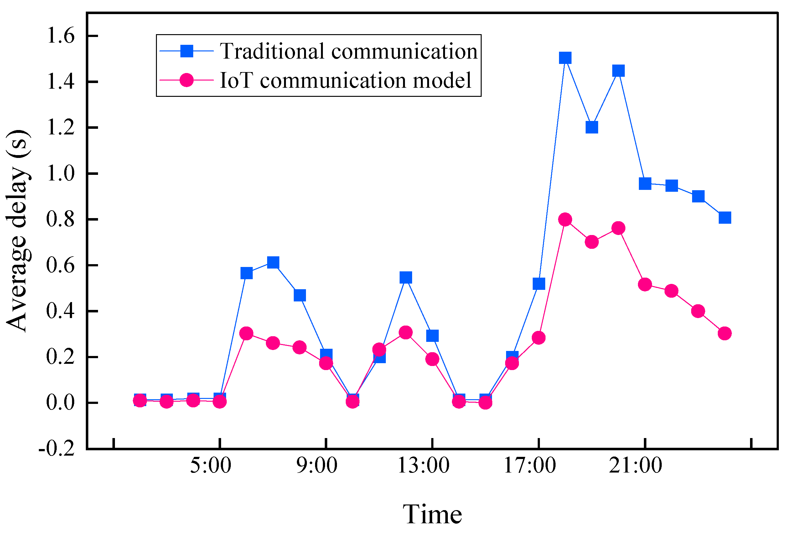
5.5.2. Transmission Reliability

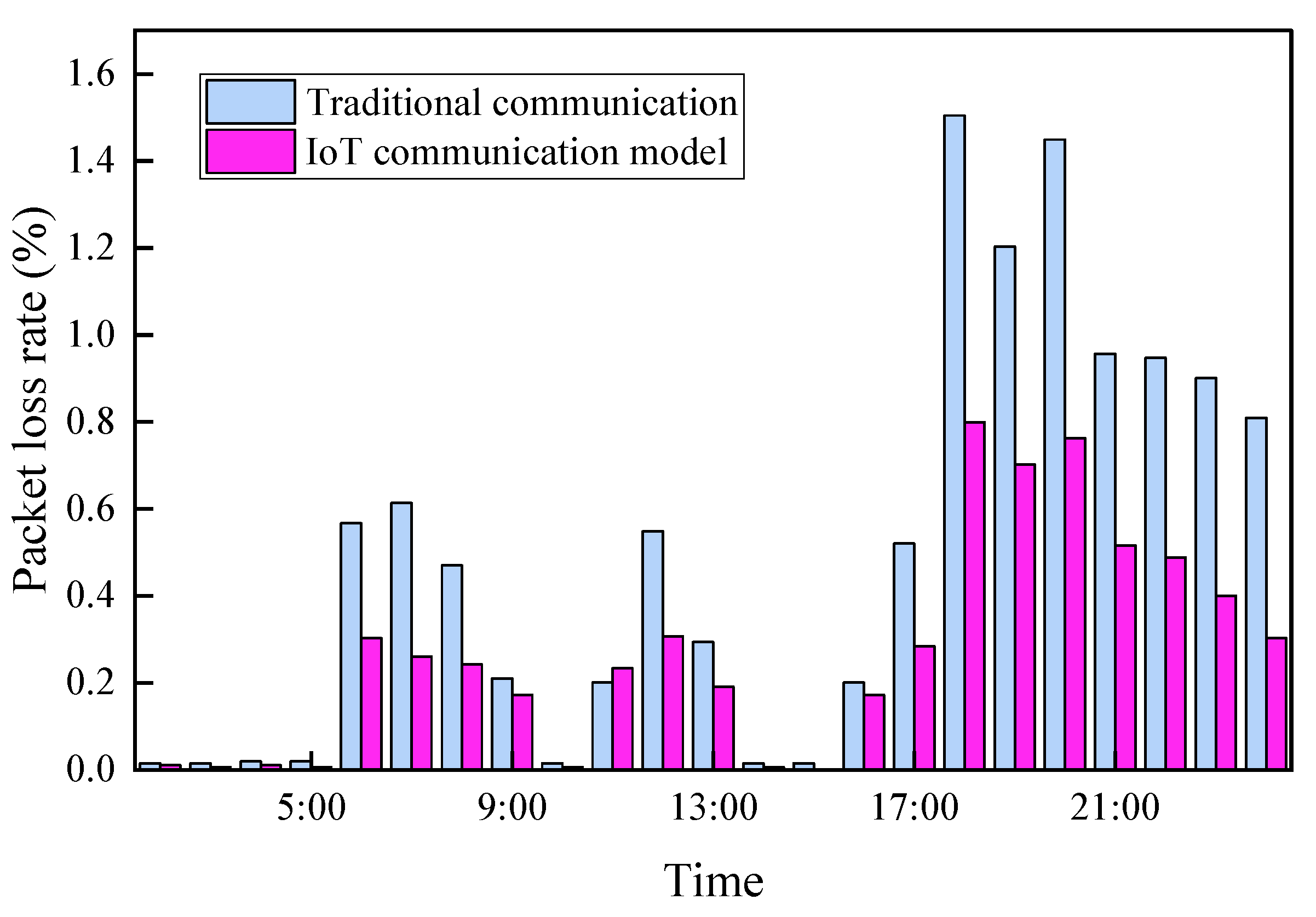
In order to provide a clearer analysis of the transmission capacity of the IoT communication model constructed in this article, the data transmission success rate is used to characterize the communication link reliability. We determined whether the IoT communication model meets the reliability requirements by examining three intervals: greater than 99.5%, between 98.0% and 99.5%, and less than 98.0%. The transceiver-related noise bandwidth to data rate ratio is 1.9. Figure 8 shows the communication transmission reliability interval analysis results. When the predicted noise transmission rate is greater than 7 dBm, the reliability of the communication link is higher than 99.5%, requiring high-reliability communication transmission data. In the reliability range between >98.0% and <99.5%, if the predicted noise transmission rate is greater than 6 dBm and less than 7 dBm, the transmission data should be lower. However, if the predicted transmission noise transmission rate is less than 6 dBm and the reliability is less than 98%, the link cannot meet the data communication requirements. Therefore, the above experimental results indicate that the model constructed in this paper can selectively restore frequency attenuation channels to flat channels, thereby reducing the impact caused by multipath fading effects.

5.5.3. Data Loss

In wireless Internet of Things communication, an effective channel guarantee mechanism is needed when the transmission layer data congestion or packet loss acceleration ratio increases sharply. To address this issue, a community with 1000 intelligent terminal data source nodes was selected. Using the IoT communication model and traditional communication systems as propagation media, the packet loss rates for each hour within a 24 h workday are shown in Figure 9. During periods of light network communication load, data transmission exhibits good performance and a relatively low packet loss rate. However, during periods of heavy load, such as between 18:00 and 24:00, the transmission packet loss rates of both models significantly increase. This system employs an IoT communication model integrated with deep learning neural networks to implement a path-optimized packet transmission mechanism. Specifically, the system dynamically calculates optimal transmission paths based on real-time network conditions. Data packets are then routed hop-by-hop along these optimized paths, effectively bypassing congestion and redundant forwarding inherent in traditional routes. The deep learning model intelligently adjusts path selection, enabling subsequent packets to circumvent network bottleneck nodes and high-loss areas. This approach significantly reduces common packet loss occurrences. During high network load conditions, this mechanism successfully preserved 0.54% of the total data volume on average. This enhancement substantially improved the integrity of communication quality monitoring data and ensured the accuracy of system data entry. By effectively addressing packet loss issues stemming from communication load fluctuations, the mechanism has markedly increased system stability and reliability.

When facing high packet loss rates, the communication transmission layer triggers a packet loss retransmission mechanism, resulting in a large number of retransmitted data packets occupying the network bandwidth and leading to an increase in data transmission latency. Figure 10 shows the transmission delay curve between the IoT communication model and traditional communication systems. These two types of delay curves both change in the same direction as network traffic, especially in heavy loads where packet loss retransmission and a slow start are the main reasons for high transmission delay. However, the IoT communication model performs well in suppressing these two triggers. Not only does it effectively preserve data packets, but it also reduces the retransmission rate. A new deep neural network window has been built to maintain large-scale transmission and avoid slow starts. During the early transmission process of the IoT communication model, the maximum delay is reduced by 35.5% compared to traditional communication systems. The average delay is 0.4 s, indicating that IoT technology provides more stable technical support for communication transmission systems.

6. Findings

As the Internet of Things (IoT) is booming, the need for reliability and efficiency in communication is becoming increasingly urgent. The rise in deep learning techniques offers new possibilities in addressing the complexity and uncertainty of IoT communications. In the future, deep learning-based reliability analyses of IoT communications will help us make significant progress in several areas. Firstly, the continuous evolution of deep learning models will make them more applicable to large-scale and diverse data in IoT communications. Improvements in neural network structure and training methods will improve communication state identification accuracy, so that potential problems can be identified in a timely manner and appropriate measures can be taken to ensure reliability. Secondly, deep learning will be more widely applied to the parameter selection optimization process. Through deep learning algorithms, the system can automatically learn the impact of different parameter configurations on the communication performance and achieve adaptive parameter adjustment. This intelligent parameter selection will make the IoT communication system more adaptive and flexible, achieving optimal performance in different environments and under varying workloads. In addition, deep learning’s powerful feature extraction capability will prompt more research to focus on deep communication data mining. By discovering the patterns and laws hidden behind the data, the system can better understand the dynamic changes in the communication environment and thus more precisely adjust the communication strategy and improve reliability. However, despite the promising prospects of the above methods, their effectiveness still has certain limitations. In extremely dynamic environments, such as when the network topology changes frequently, nodes are highly heterogeneous, or sensor failure rates are high, deep learning models may have difficulty maintaining stable performance. In addition, when the training data is insufficient or biased, the model may not accurately reflect the actual communication status, leading to misjudgment and policy failure.

7. Conclusions

This article focuses on reliability analysis and parameter selection to construct an IoT communication model based on deep learning. We analyzed communication reliability with regard to different parameter dimensions in practical analysis. Our conclusions are as follows:

(1)

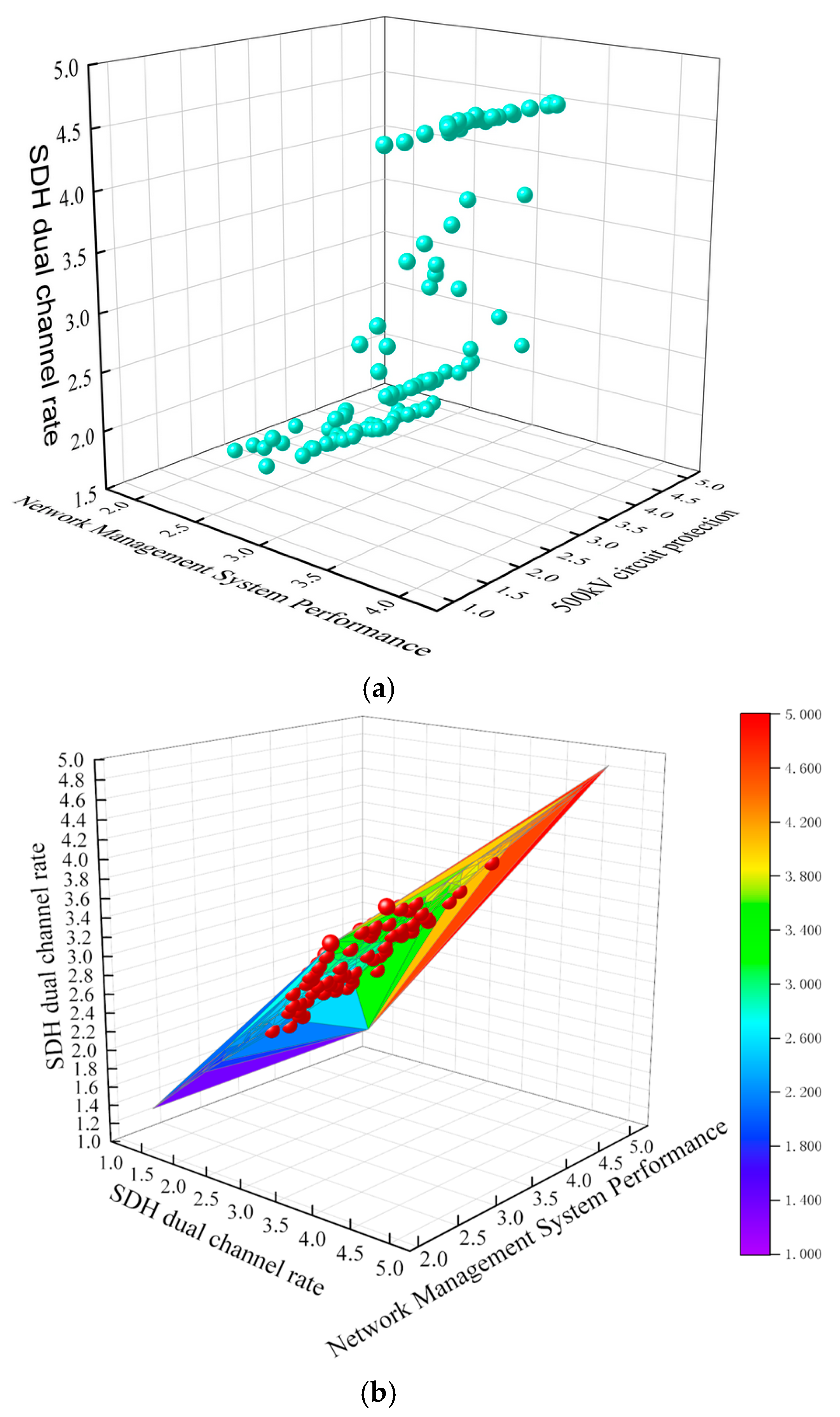
After reducing data dimensionality through the communication model constructed in this article, a two-dimensional feature plane can be obtained and the running data can be distinguished on the reliability feature plane.

(2)

Our IoT communication model, which can quickly and efficiently switch between training and testing sets, converges to 0 when the signal-to-noise ratio is 90 dB. The success rate of cross zone switching is greater than 99.6%, meeting the requirement of current wireless communication system technologies (success rate ≥ 99.5%).

(3)

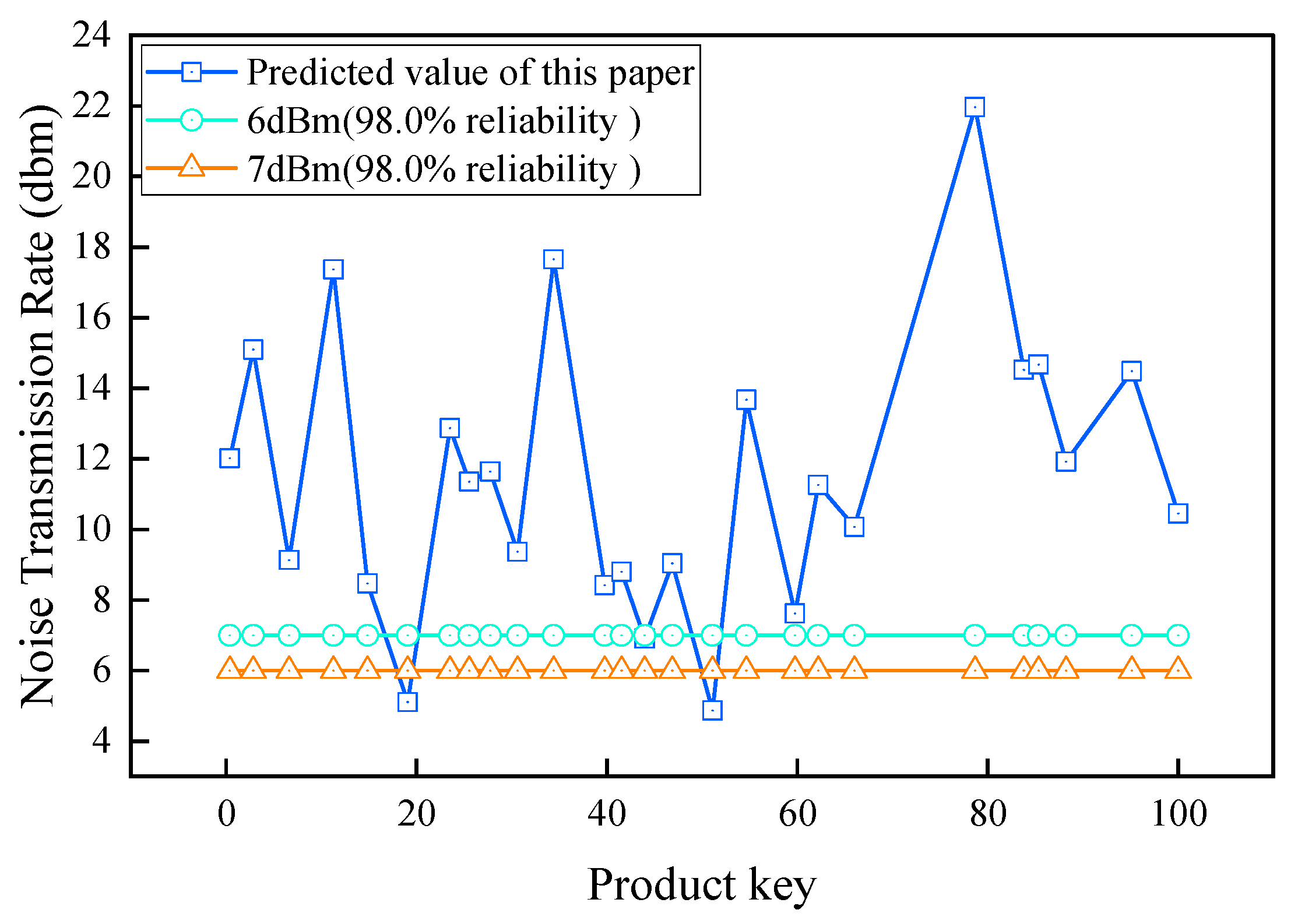
When the predicted noise transmission rate is greater than 6 dBm and greater than 7 dBm, the reliability is greater than 98.0% and less than 99.5%, meeting the communication reliability requirements.

Future research should further investigate the model’s performance in more complex and dynamic IoT environments, particularly its applicability in scenarios with frequent network topology changes, high node heterogeneity, and resource-constrained devices. Additionally, efforts should be enhanced to address data bias and incompleteness issues encountered in practical applications, thereby improving the model’s robustness and generalization capabilities.

References

1. Uzoka, A.; Cadet, E.; Ojukwu, P.U. The role of telecommunications in enabling Internet of Things (IoT) connectivity and applications. Compr. Res. Rev. Sci. Technol. 2024, 2, 055–073. [Google Scholar] [CrossRef]
2. Allioui, H.; Mourdi, Y. Exploring the full potentials of IoT for better financial growth and stability: A comprehensive survey. Sensors 2023, 23, 8015. [Google Scholar] [CrossRef] [PubMed]
3. Shen, M.; Ye, K.; Liu, X.; Zhu, L.; Kang, J.; Yu, S.; Li, Q.; Xu, K. Machine learning-powered encrypted network traffic analysis: A comprehensive survey. IEEE Commun. Surv. Tutor. 2022, 25, 791–824. [Google Scholar] [CrossRef]
4. Illi, E.; Qaraqe, M.; Althunibat, S.; Alhasanat, A.; Alsafasfeh, M.; De Ree, M.; Al-Kuwari, S. Physical layer security for authentication, confidentiality, and malicious node detection: A paradigm shift in securing IoT networks. IEEE Commun. Surv. Tutor. 2023, 26, 347–388. [Google Scholar] [CrossRef]
5. Macriga, G.A.; Fathila, M.F.; Helen, A.; Rijwana, R.; Syed, H.H. Automatic identification and monitoring system for fisherman based on narrowband and internet of things communications systems. SSRN Electron. J. 2019, 6, 303–307. [Google Scholar]
6. Ramadhan, A.J. Smart glasshouse system supported by global system for mobile communications and internet of things: Case study: Tomato plant. J. Eng. Sci. Technol. 2020, 15, 3067–3081. [Google Scholar]
7. Roseela, J.A.; Godhavari, T.; Narayanan, R.M.; Madhuri, P.L. Design and deployment of IoT based underwater wireless communication system using electronic sensors and materials. Mater. Today Proc. 2021, 45, 6229–6233. [Google Scholar] [CrossRef]
8. Dong, N. A malicious intrusion detection model of network communication in cloud data center. J. Interconnect. Netw. 2022, 22, 2141023. [Google Scholar] [CrossRef]
9. Agrawal, N.K.; Alam, S.; Raghav, H. Osi model: The basics structure of network communication. Int. J. Recent Technol. Eng. 2021, 9, 66–69. [Google Scholar] [CrossRef]
10. Mahler, T.; Kowalewski, J.; Nub, B.; Richt, C.; Mayer, J.; Zwick, T. Channel measurement based antenna synthesis for mobile automotive mimo communication systems. Prog. Electromagn. Res. B 2017, 72, 1–16. [Google Scholar] [CrossRef]
11. Deepa, A.; Marimuthu, C.N. A high speed vlsi architecture of a pipelined reed solomon encoder for data storage in communication systems. Asian J. Res. Soc. Sci. Humanit. 2017, 7, 228–238. [Google Scholar] [CrossRef]
12. Samyuel, N.B.; Shimray, B.A. Securing iot device communication against network flow attacks with recursive internetworking architecture (rina)-sciencedirect. ICT Express 2021, 7, 110–114. [Google Scholar] [CrossRef]
13. Suma, V. Wearable iot based distributed framework for ubiquitous computing. J. Ubiquitous Comput. Commun. Technol. 2021, 3, 23–32. [Google Scholar] [CrossRef]
14. Babu, C.; Kumar, D.D.; Kumar, K.; Reddy, K.J.; Sudha, R. Power monitoring and control system for medium voltage smart grid using iot. IOP Conf. Ser.: Mater. Sci. Eng. 2020, 906, 012007. [Google Scholar] [CrossRef]
15. Moriyama, M.; Takizawa, K.; Tezuka, H.; Kojima, F. Experimental evaluation of stbc and cdd for reliable downlink communication. IEICE Commun. Express 2020, 9, 312–317. [Google Scholar] [CrossRef]
16. Liaskos, C.; Pyrialakos, G.G.; Pitilakis, A.; Tsioliaridou, A.; Christodoulou, M.; Kantartzis, N.; Ioannidis, S.; Pitsillides, A.; Akyildiz, I.F. Integrating Software-Defined Metasurfaces into Wireless Communication Systems: Design and Prototype Evaluation. In Proceedings of the 2022 IEEE Symposium on Computers and Communications (ISCC), Rhodes, Greece, 30 June–3 July 2022; pp. 1–6. [Google Scholar]
17. Kanno, S.; Imaike, T.; Otani, A. Study of radio communication evaluation system using under-sampling. IEEJ Trans. Fundam. Mater. 2018, 138, 180–185. [Google Scholar] [CrossRef]
18. Gao, L.; Chen, L.; Yu, F. The research on effectiveness evaluation of mobile broadband wireless communication system. J. Phys. Conf. Ser. 2020, 1634, 012061. [Google Scholar] [CrossRef]
19. Zang, Y.; Zhenming, Y.; Xu, K.; Chen, M.; Yang, S.; Chen, H.W. Data-driven fiber model based on the deep neural network with multi-head attention mechanism. Opt. Express 2022, 30, 46626–46648. [Google Scholar] [CrossRef] [PubMed]
20. Cha, Y.J.; Choi, W.; Büyüköztürk, O. Deep learning-based crack damage detection using convolutional neural networks. Comput. Aided Civ. Infrastruct. Eng. 2017, 32, 361–378. [Google Scholar] [CrossRef]
21. Lee, C.S.; Baughman, D.M.; Lee, A.Y. Deep learning is effective for classifying normal versus age-related macular degeneration oct images. Ophthalmol. Retin. 2017, 1, 322–327. [Google Scholar] [CrossRef] [PubMed]
22. Kuang, C. Research on network traffic anomaly detection method based on deep learning. J. Phys. Conf. Ser. 2021, 1861, 012007. [Google Scholar] [CrossRef]
23. Li, P.; Cai, J. Research on image recognition from wireless sensor data based on deep learning. CE Ca 2017, 42, 2607–2612. [Google Scholar]
24. Zhang, A.; Wang, K.C.; Li, B.; Yang, E.; Dai, X.; Peng, Y.; Fei, Y.; Liu, Y.; Li, J.Q.; Chen, C. Automated pixel-level pavement crack detection on 3d asphalt surfaces using a deep-learning network. Comput.-Aided Civ. Infrastruct. Eng. 2017, 32, 805–819. [Google Scholar] [CrossRef]
25. Zhang, L.; Chen, B.; Li, H.; Liu, Y. Deep neural network-based adaptive zero-velocity detection for pedestrian navigation system. Electron. Lett. 2022, 58, 28–31. [Google Scholar] [CrossRef]
26. Ilbeigi, M.; Morteza, A.; Ehsani, R. Emergency management in smart cities: Infrastructure-less communication systems. Constr. Res. Congr. 2022, 2022, 263–271. [Google Scholar]
27. Kim, W.S.; Kim, J.K.; Park, B.S.; Kwan-Jung Oh Seo, Y.H. Phase-only hologram video compression using a deep neural network for up-scaling and restoration. Appl. Opt. 2022, 61, 10644–10657. [Google Scholar] [CrossRef] [PubMed]
28. Du, R.; Magnusson, S.; Fischione, C. The Internet of Things as a deep neural network. IEEE Commun. Mag. 2020, 58, 20–25. [Google Scholar] [CrossRef]
29. Uryvsky, L.; Gerstacker, W.; Moshynska, A.; Osypchuk, S.; Yatsyshyn, O. Research and implementation of iot projects for environment parameters and energy resource metering. Inf. Telecommun. Sci. 2020, 1, 27–34. [Google Scholar] [CrossRef]
30. Kovtun, V.; Izonin, I.; Gregus, M. Formalization of the metric of parameters for quality evaluation of the subject-system interaction session in the 5g-iot ecosystem. Alex. Eng. J. 2022, 61, 7941–7952. [Google Scholar] [CrossRef]
Figure 1. Deep neural network structure.
Eng 06 00171 g001
Figure 2. Neuronal structure.
Eng 06 00171 g002
Figure 3. Basic structure of the internet communication model.
Eng 06 00171 g003
Figure 4. Communication Reliability Parameter Architecture.
Eng 06 00171 g004
Figure 5. Comparison of communication reliability data before and after downgrading. (a) Communication 3D reliability characterization data before downscaling. (b) Communication 3D reliability characterization data after dimensionality re-duction.
Eng 06 00171 g005
Figure 6. Mean square error performance.
Eng 06 00171 g006
Figure 7. Cost of fault recovery time.
Eng 06 00171 g007
Figure 8. Reliability interval analysis results.
Eng 06 00171 g008
Figure 9. Hourly packet loss rate over a 24 h working day.
Eng 06 00171 g009
Figure 10. Average delay statistics results.
Eng 06 00171 g010