
Enhancing Software Defect Prediction Using Ensemble Techniques and Diverse Machine Learning Paradigms

 , , ,
, , ,  and
and 
Abstract
1. Introduction
- To evaluate the effectiveness of ensemble methods and machine learning algorithms, primarily focusing on semi-supervised and self-supervised learning, in predicting software defects;
- To compare the performance of these methods and recommend the most suitable model for predicting software defects using a specific dataset.
2. Literature Review
3. Methodology
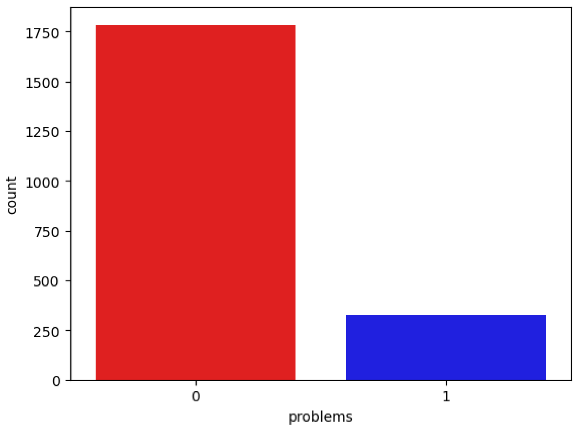
3.1. Dataset
3.2. Data Prepossessing
3.3. ML Algorithms
- Logistic Regression (LR): By using the data to fit a linear equation observed, the LR method establishes the relationship between independent and dependent features [20]. For LR, the activation function is explained as:Here, e = natural logarithm base and value = the number that one wants to change.Logistic Regression (LR)—Sigmoid Function (SF); Here, m denotes the value of input, n is the output that is predicted, is the term of intercept, and is the coefficient of the input value (m).
- Random Forest (RF): Multiple decision trees are built by the machine learning algorithm RF, which then aggregates the predictions by voting or averaging them [21].Here, is the ith decision tree’s prediction, N is the forest’s total tree count, and is the ensemble prediction.
- Decision Tree (DT): The DT algorithm partitions data based on features to predict outcomes. Its equation Z(m) is represented by recursive splitting, optimizing purity measures like Gini impurity or entropy [22]. The Gini impurity measure is given byHere, e represents the total number of classes, and shows the percentage of samples in class i in set m. The entropy measure is given bywith m having e classes, where the percentage of samples in class i is shown by .
- Gradient Boosting (GB): GB is an algorithm of machine learning that iteratively improves weak learners by minimizing a loss function. This algorithm is represented as an iterative process of combining weak learners (m) to minimize the overall loss function, typically through gradient descent. The function at each stage m in the gradient boosting algorithm is represented as m combines weak learners to approximate the true functions [23].
- Support Vector Machines (SVMs): SVM is the powerful supervised learning method for regression and classification in order to choose the best hyperplane for maximizing the class margin. The decision boundary in SVM is represented as, where represents weights, denotes input features, and b is the term of bias [24].
- K-Nearest Neighbors (KNN): The KNN algorithm classifies data items depending on the majority class of the k nearest neighbors. If a new data point m is given, the KNN classifier estimates the class label of k’s nearest neighbors by using the majority vote.Here, the number of features is n, and the ith training instance is . Choose the k locations with the shortest distances to determine the k nearest neighbors [22].
- AdaBoost Classifier (AC): The AC algorithm incorporates weak learners to create a powerful classifier by iterative adjusting weights. Its mathematical equation iswhere are the weights and are weak learners [25].
- Gaussian Classifier (GC): A GC is a common probabilistic model assuming features’ normal distribution, often applied to classification tasks with continuous features presumed to be independent given class labels [26].Let m be the feature of the vector and n be the label of the class. The Gaussian naive Bayes classifier determines the posterior probability using Bayes’ theorem:where = the posterior probability of class n given characteristics m, = the probability of seeing features m for class n, = class n’s prior probability, and = the probability of focusing on features m, also known as the evidence.
- Quadratic Discriminant Analysis (QDA): Assuming that every class has a multivariate normal distribution, the QDA classification algorithm calculates a unique covariance matrix for each class. Unlike Gaussian NB, QDA does not assume equal covariance matrices across classes [27]. In the case of class n and a feature vector m, the probability density function is as follows:where f is the feature number, is the class n mean vector, and is the class n covariance matrix. Assigning an input vector m to the class with the highest posterior probability is the decision rule for classifying it:
- Ridge Classifier: This is commonly used in scenarios where there’s multicollinearity among the features. The ridge classifier intends to minimize the goal function listed below:Here, the feature matrix is represented by M, the target vector by n, the coefficient vector by w, and the regularization parameter by [27].
4. Experimental Result and Analysis
4.1. Evaluation Metrics
- Additional Metrics:
- –
- Accuracy: It evaluates the model’s overall accuracy. In accuracy, the higher value is the better outcome.
- –
- Recall: It calculates the percentage of actual positives among all genuine positive predictions. Higher is better, especially in situations where missing positives costly.
- –
- Precision: Of all positive forecasts, it calculates the percentage of real positive predictions. Higher values are better, especially when false positives are unwanted or expensive.
- –
- F1-score: A balance between precision and recall is provided by the harmonic mean of the two. Since it shows a good balance between recall and precision, higher is preferable.
- Regression and Error Metrics:
- –
- False Positive Rate (F-Positive): This calculates the proportion of incorrectly negatives classified as positives. For F-Positive, lower is preferable.
- –
- False Negative Rate (F-Negative): This measures the proportion of positives incorrectly classified as negatives. Lower is better, as it means fewer actual positives are missed.
- –
- Negative Predictive Value (N-Predictive): This calculates the ratio of true negatives among all predicted negatives. Higher is better, as it indicates the model is accurately identifying negatives.
- –
- False Discovery Rate (F-Discovery Rate): This calculates the ratio of false positives among all predicted positives. Lower is better, as it means fewer incorrect predictions among the positive predictions.
- –
- Mean Absolute Error (MAE): This calculates the average amount of discrepancies between expected and actual values, without taking instructions. Lower is better, as it means the predictions are closer to the actual values.
- –
- R-squared Error (RSE): This calculates the standard deviation of residuals (prediction errors). It reflects the unexplained variance in the data. Lower is better, as it indicates the model fits the data more accurately with fewer errors.
- –
- Root Mean Squared Error (RMSE): It calculates the square root of average squared deviations between actual and expected values. Compared to MAE, it penalizes major mistakes more. Lower is better, as it means fewer prediction errors, particularly penalizing larger deviations.
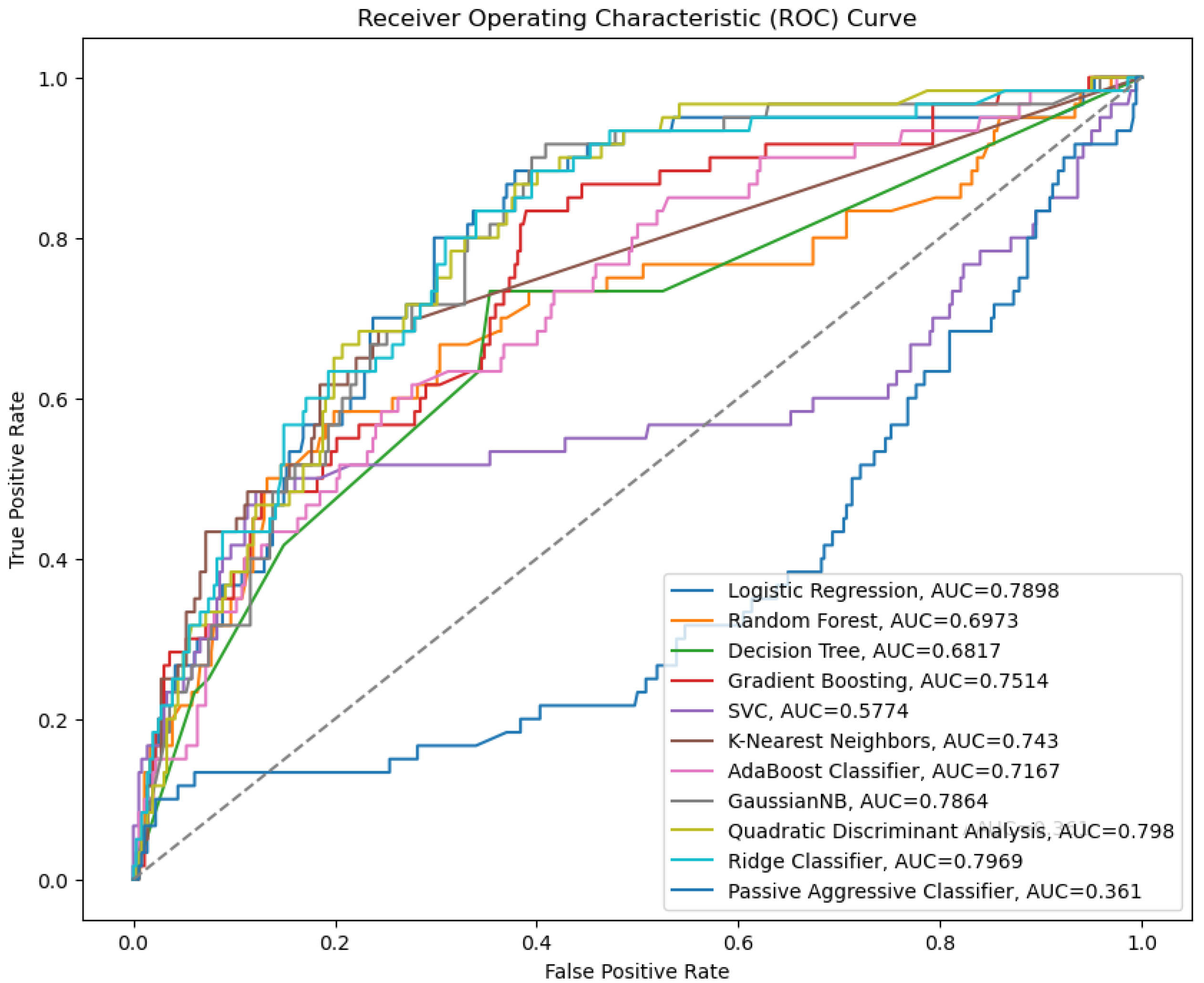
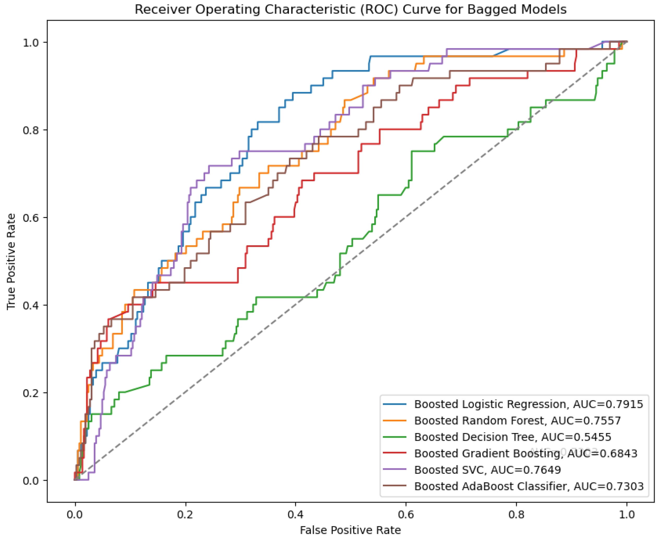
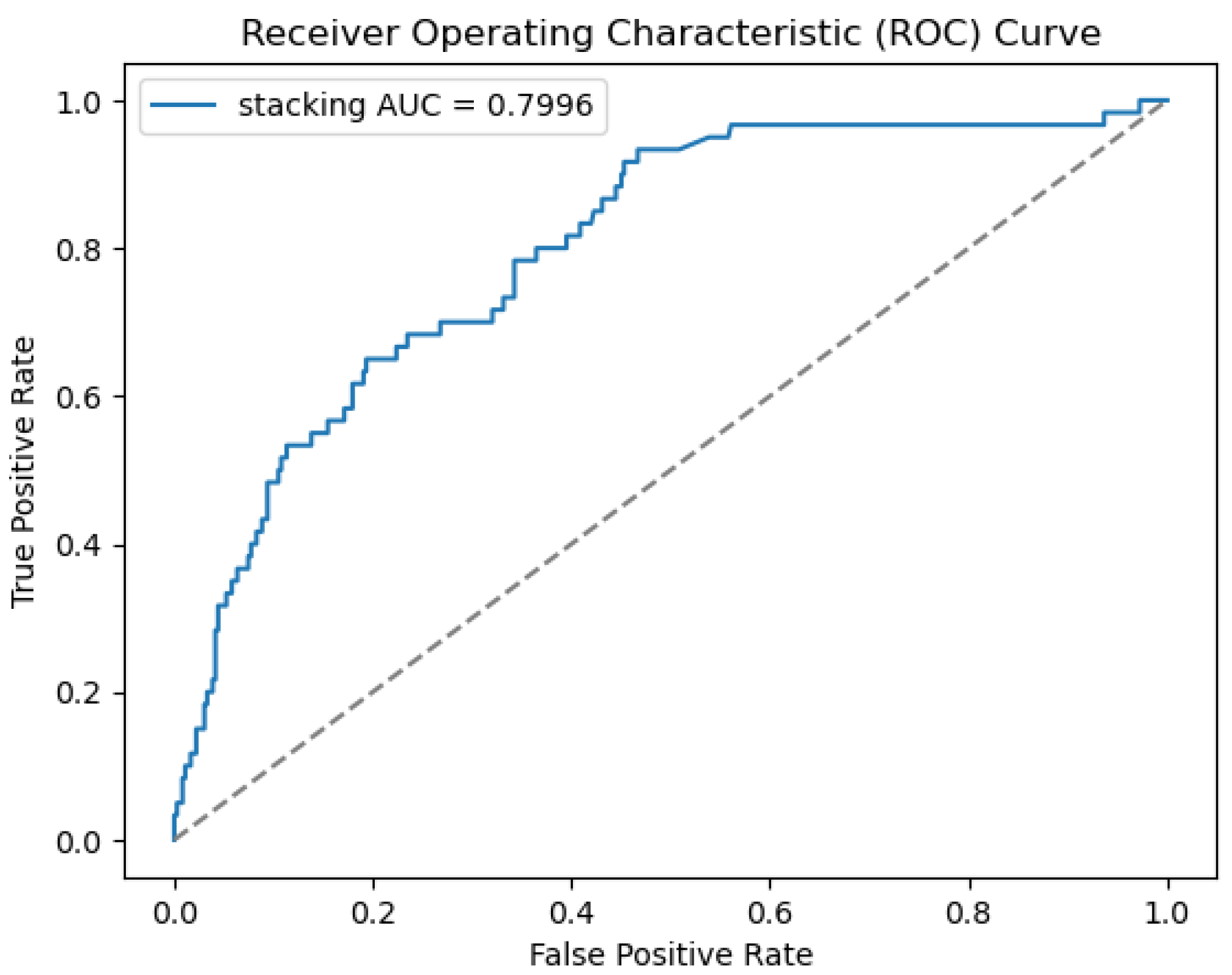
4.2. Performance Analysis
5. Conclusions
Author Contributions
Funding
Institutional Review Board Statement
Informed Consent Statement
Data Availability Statement
Conflicts of Interest
References
- Fan, C.; Lei, Y.; Sun, Y.; Mo, L. Novel transformer-based self-supervised learning methods for improved HVAC fault diagnosis performance with limited labeled data. Energy 2023, 278, 127972. [Google Scholar] [CrossRef]
- Petrovic, A.; Jovanovic, L.; Bacanin, N.; Antonijevic, M.; Savanovic, N.; Zivkovic, M.; Gajic, V. Exploring metaheuristic optimized machine learning for software defect detection on natural language and classical datasets. Mathematics 2024, 12, 2918. [Google Scholar] [CrossRef]
- Ramírez-Sanz, J.M.; Maestro-Prieto, J.A.; Arnaiz-González, Á.; Bustillo, A. Semi-supervised learning for industrial fault detection and diagnosis: A systemic review. ISA Trans. 2023, 143, 255–270. [Google Scholar] [CrossRef] [PubMed]
- Albayati, M.G.; Faraj, J.; Thompson, A.; Patil, P.; Gorthala, R.; Rajasekaran, S. Semi-supervised machine learning for fault detection and diagnosis of a rooftop unit. Big Data Min. Anal. 2023, 6, 170–184. [Google Scholar] [CrossRef]
- De Vries, S.; Thierens, D. A reliable ensemble-based approach to semi-supervised learning. Knowl.-Based Syst. 2021, 215, 106738. [Google Scholar] [CrossRef]
- Askari, B.; Cavone, G.; Carli, R.; Grall, A.; Dotoli, M. A semi-supervised learning approach for fault detection and diagnosis in complex mechanical systems. In Proceedings of the 2023 IEEE 19th International Conference on Automation Science and Engineering (CASE), Auckland, New Zealand, 26–30 August 2023; pp. 1–6. [Google Scholar] [CrossRef]
- Wang, H.; Liu, Z.; Ge, Y.; Peng, D. Self-supervised signal representation learning for machinery fault diagnosis under limited annotation data. Knowl.-Based Syst. 2022, 239, 107978. [Google Scholar] [CrossRef]
- Wang, X.; Kihara, D.; Luo, J.; Qi, G.-J. Enaet: A self-trained framework for semi-supervised and supervised learning with ensemble transformations. IEEE Trans. Image Process. 2021, 30, 1639–1647. [Google Scholar] [CrossRef]
- Mehmood, I.; Shahid, S.; Hussain, H.; Khan, I.; Ahmad, S.; Rahman, S.; Ullah, N.; Huda, S. A novel approach to improve software defect prediction accuracy using machine learning. IEEE Access 2023, 11, 63579–63597. [Google Scholar] [CrossRef]
- Md Rashedul Islam, M.B.; Akhtar, M.N. Recursive approach for multiple step- ahead software fault prediction through long short-term memory (LSTM). J. Discret. Math. Sci. Cryptogr. 2022, 25, 2129–2138. [Google Scholar] [CrossRef]
- Han, T.; Xie, W.; Pei, Z. Semi-supervised adversarial discriminative learning approach for intelligent fault diagnosis of wind turbine. Inf. Sci. 2023, 648, 119496. [Google Scholar] [CrossRef]
- Qi, G.-J.; Luo, J. Small data challenges in big data era: A survey of recent progress on unsupervised and semi-supervised methods. IEEE Trans. Pattern Anal. Mach. Intell. 2022, 44, 2168–2187. [Google Scholar] [CrossRef] [PubMed]
- Šikić, L.; Afrić, P.; Kurdija, A.S.; Šilić, M. Improving software defect prediction by aggregated change metrics. IEEE Access 2021, 9, 19391–19411. [Google Scholar] [CrossRef]
- Meng, A.; Cheng, W.; Wang, J. An integrated semi-supervised software defect prediction model. J. Internet Technol. 2023, 24, 1307–1317. [Google Scholar] [CrossRef]
- Begum, M.; Rony, J.H.; Islam, M.R.; Uddin, J. A long-term software fault prediction model using box-cox and linear regression. J. Inf. Syst. Telecommun. 2023, 11, 222–233. [Google Scholar]
- ul Haq, Q.M.; Arif, F.; Aurangzeb, K.; ul Ain, N.; Khan, J.A.; Rubab, S.; Anwar, M.S. Identification of software bugs by analyzing natural language-based requirements using optimized deep learning features. Comput. Mater. Contin. 2024, 78, 4379–4397. [Google Scholar]
- Villoth, J.P.; Zivkovic, M.; Zivkovic, T.; Abdel-salam, M.; Hammad, M.; Jovanovic, L.; Bacanin, N. Two-tier deep and machine learning approach optimized by adaptive multi-population firefly algorithm for software defects prediction. Neurocomputing 2025, 630, 129695. [Google Scholar] [CrossRef]
- Begum, M.; Shuvo, M.H.; Ashraf, I.; Mamun, A.A.; Uddin, J.; Samad, M.A. Software defects identification: Results using machine learning and explainable artificial intelligence techniques. IEEE Access 2023, 11, 132750–132765. [Google Scholar] [CrossRef]
- Rahman, S. Soft Defect Dataset. Kaggle. 2019. Available online: https://www.kaggle.com/datasets/sazid28/soft-defect/data (accessed on 10 July 2025).
- Tapu Rayhan, M.H.N.S. Ayesha Siddika: Social media emotion detection and analysis system using cutting-edge artificial intelligence techniques. In Proceedings of the 9th International Congress on Information and Communication Technology (ICICT 2024), London, UK, 19–22 February 2024. [Google Scholar]
- Breiman, L. Random forests. Mach. Learn. 2001, 45, 5–32. [Google Scholar] [CrossRef]
- Cover, T.; Hart, P. Nearest neighbor pattern classification. IEEE Trans. Inf. Theory 1967, 13, 21–27. [Google Scholar] [CrossRef]
- Friedman, J.H. Greedy function approximation: A gradient boosting machine. Ann. Stat. 2001, 29, 1189–1232. [Google Scholar] [CrossRef]
- Cortes, C.; Vapnik, V. Support-vector networks. Mach. Learn. 1995, 20, 273–297. [Google Scholar] [CrossRef]
- Freund, Y.; Schapire, R.E. A decision-theoretic generalization of on-line learning and an application to boosting. J. Comput. Syst. Sci. 1997, 55, 119–139. [Google Scholar] [CrossRef]
- Bishop, C.M. Pattern Recognition and Machine Learning; Springer: New York, NY, USA, 2006. [Google Scholar]
- Hastie, T.; Tibshirani, R.; Friedman, J. The Elements of Statistical Learning: Data Mining, Inference, and Prediction; Springer: New York, NY, USA, 2009. [Google Scholar]


| SN | Classification Report | LR | RF | DT | GB | SVM | KNN | AC | GT | QDA | RC | PAC |
|---|---|---|---|---|---|---|---|---|---|---|---|---|
| 0 | Accuracy | 86.50 | 88.31 | 84.37 | 90.10 | 86.30 | 85.10 | 89.60 | 86.00 | 84.20 | 86.50 | 85.80 |
| 1 | Precision | 0.98 | 0.96 | 0.95 | 0.95 | 0.98 | 0.95 | 0.98 | 0.89 | 0.93 | 0.98 | 0.99 |
| 2 | Specificity | 0.57 | 0.47 | 0.42 | 0.46 | 0.56 | 0.46 | 0.47 | 0.32 | 0.43 | 0.58 | 0.50 |
| 3 | F1-score | 0.69 | 0.62 | 0.57 | 0.64 | 0.68 | 0.61 | 0.64 | 0.45 | 0.70 | 0.64 | 0.64 |
| 4 | Recall | 0.89 | 0.89 | 0.88 | 0.89 | 0.88 | 0.89 | 0.87 | 0.89 | 0.90 | 0.89 | 0.87 |
| 5 | F-Positive | 0.44 | 0.54 | 0.59 | 0.55 | 0.45 | 0.55 | 0.54 | 0.42 | 0.58 | 0.43 | 0.05 |
| 6 | F-Negative | 0.12 | 0.12 | 0.10 | 0.12 | 0.10 | 0.12 | 0.10 | 0.12 | 0.08 | 0.10 | 0.05 |
| 7 | N-Predictive | 0.22 | 0.24 | 0.25 | 0.27 | 0.17 | 0.27 | 0.12 | 0.32 | 0.34 | 0.22 | 0.11 |
| 8 | F-Discovery Rate | 0.03 | 0.05 | 0.06 | 0.05 | 0.02 | 0.05 | 0.01 | 0.06 | 0.05 | 0.03 | 0.01 |
| 9 | MAE | 0.14 | 0.15 | 0.16 | 0.15 | 0.13 | 0.12 | 0.13 | 0.16 | 0.15 | 0.14 | 0.15 |
| 10 | RSE | 0.11 | 0.21 | 0.29 | 0.23 | 0.13 | 0.23 | 0.19 | 0.46 | 0.31 | 0.14 | 0.17 |
| 11 | RMSE | 0.37 | 0.39 | 0.40 | 0.39 | 0.38 | 0.39 | 0.39 | 0.45 | 0.40 | 0.37 | 0.38 |
| Model | Accuracy (%) | 95% CI+/− | F1-Score | 95% CI+/− | Significant vs. GB (p-Value) |
|---|---|---|---|---|---|
| GB | 90.10 | 1.12 | 0.64 | 0.03 | - |
| RF | 88.31 | 1.45 | 0.62 | 0.04 | 0.027 |
| QDA | 84.20 | 1.89 | 0.70 | 0.02 | 0.039 |
| SVM | 86.30 | 1.22 | 0.68 | 0.03 | 0.068 |
| LR | 86.50 | 1.30 | 0.69 | 0.02 | 0.073 |
| SN | Classification Report | Autoencoder | S3VM | GAN |
|---|---|---|---|---|
| 0 | Accuracy | 0.84 | 0.85 | 0.87 |
| 1 | Precision | 0.58 | 0.60 | 0.62 |
| 2 | Specificity | 1.00 | 0.98 | 0.97 |
| 3 | F1-score | 0.52 | 0.60 | 0.86 |
| 4 | Recall | 0.56 | 0.82 | 0.96 |
| 5 | F-Positive | 0.03 | 0.02 | 0.03 |
| 6 | F-Negative | 1.00 | 0.82 | 0.80 |
| 7 | N-Predictive | 0.84 | 0.87 | 0.87 |
| 8 | F-Discovery Rate | 0.41 | 0.41 | 0.40 |
| 9 | MAE | 0.16 | 0.16 | 0.15 |
| 10 | RSE | 0.31 | −0.20 | 0.35 |
| 11 | RMSE | 0.29 | 0.38 | 0.00 |
| SN | Classification Report | Autoencoder | SimCLR | BYOL |
|---|---|---|---|---|
| 0 | Accuracy | 83.65 | 85.86 | 85.07 |
| 1 | Precision | 0.58 | 0.68 | 0.62 |
| 2 | Specificity | 1.00 | 0.97 | 0.96 |
| 3 | F1-score | 0.54 | 0.67 | 0.61 |
| 4 | Recall | 0.78 | 0.82 | 0.80 |
| 5 | F-Positive | 0.02 | 0.03 | 0.01 |
| 6 | F-Negative | 0.22 | 0.14 | 0.38 |
| 7 | N-Predictive | 0.80 | 0.87 | 0.85 |
| 8 | F-Discovery Rate | 0.41 | 0.42 | 0.38 |
| 9 | MAE | 0.16 | 0.14 | 0.14 |
| 10 | RSE | 0.19 | 0.11 | 0.13 |
| 11 | RMSE | 0.40 | 0.39 | 0.38 |
Disclaimer/Publisher’s Note: The statements, opinions and data contained in all publications are solely those of the individual author(s) and contributor(s) and not of MDPI and/or the editor(s). MDPI and/or the editor(s) disclaim responsibility for any injury to people or property resulting from any ideas, methods, instructions or products referred to in the content. |
© 2025 by the authors. Licensee MDPI, Basel, Switzerland. This article is an open access article distributed under the terms and conditions of the Creative Commons Attribution (CC BY) license (https://creativecommons.org/licenses/by/4.0/).
Share and Cite
Siddika, A.; Begum, M.; Al Farid, F.; Uddin, J.; Karim, H.A. Enhancing Software Defect Prediction Using Ensemble Techniques and Diverse Machine Learning Paradigms. Eng 2025, 6, 161. https://doi.org/10.3390/eng6070161
Siddika A, Begum M, Al Farid F, Uddin J, Karim HA. Enhancing Software Defect Prediction Using Ensemble Techniques and Diverse Machine Learning Paradigms. Eng. 2025; 6(7):161. https://doi.org/10.3390/eng6070161
Chicago/Turabian StyleSiddika, Ayesha, Momotaz Begum, Fahmid Al Farid, Jia Uddin, and Hezerul Abdul Karim. 2025. "Enhancing Software Defect Prediction Using Ensemble Techniques and Diverse Machine Learning Paradigms" Eng 6, no. 7: 161. https://doi.org/10.3390/eng6070161
APA StyleSiddika, A., Begum, M., Al Farid, F., Uddin, J., & Karim, H. A. (2025). Enhancing Software Defect Prediction Using Ensemble Techniques and Diverse Machine Learning Paradigms. Eng, 6(7), 161. https://doi.org/10.3390/eng6070161