Abstract
In today’s fast-paced world of software development, it is essential to ensure that programs run smoothly without any issues. When dealing with complex applications, the objective is to predict and resolve problems before they escalate. The prediction of software defects is a crucial element in maintaining the stability and reliability of software systems. This research addresses this need by combining advanced techniques (ensemble techniques) with seventeen machine learning algorithms for predicting software defects, categorised into three types: semi-supervised, self-supervised, and supervised. In supervised learning, we mainly experimented with several algorithms, including random forest, k-nearest neighbors, support vector machines, logistic regression, gradient boosting, AdaBoost classifier, quadratic discriminant analysis, Gaussian training, decision tree, passive aggressive, and ridge classifier. In semi-supervised learning, we tested are autoencoders, semi-supervised support vector machines, and generative adversarial networks. For self-supervised learning, we utilized are autoencoder, simple framework for contrastive learning of representations, and bootstrap your own latent. After comparing the performance of each machine learning algorithm, we identified the most effective one. Among these, the gradient boosting AdaBoost classifier demonstrated superior performance based on an accuracy of 90%, closely followed by the AdaBoost classifier at 89%. Finally, we applied ensemble methods to predict software defects, leveraging the collective strengths of these diverse approaches. This enables software developers to significantly enhance defect prediction accuracy, thereby improving overall system robustness and reliability.
1. Introduction
In modern software development, the quest for reliability and robustness is the cornerstone of success. As the complexity of software systems increases, identifying and rectifying faults has become a paramount concern for developers and stakeholders alike. The ability to detect defects efficiently and effectively not only ensures other user experiences but also mitigates potential risks and liabilities associated with system failures [1]. In this pursuit, the use of various methodologies and techniques has emerged as a key strategy. Supervised learning, long hailed as a stalwart in predictive analytics, has found its application in software defect prediction by leveraging labeled data to train algorithms to recognize patterns indicative of defects. However, supervised learning has limitations, specifically in situations where labeled data is not available or expensive to obtain, which has prompted the exploration of alternative approaches [2]. Enter semi-supervised learning, which capitalizes on a blend of labeled and unlabeled data to improve prediction accuracy, making it particularly well-suited for domains where labeled data is limited [3]. Additionally, the paradigm of self-supervised learning has garnered interest because of its power to obtain meaningful representations from unlabeled data, thus circumventing the need for extensive labeling efforts altogether [4]. Moreover, recognizing the inherent variability and unpredictability of software systems, ensemble methods have emerged as a robust strategy for defect prediction. By combining the outputs of multiple base detectors, ensemble methods offer improved performance and resilience against noise and outliers, thereby enhancing the reliability of defect prediction systems. This study makes several significant contributions to the prediction of software defects. These contributions collectively enhance the most advanced in harnessing machine learning and ensemble methods’ power, as follows:
- To evaluate the effectiveness of ensemble methods and machine learning algorithms, primarily focusing on semi-supervised and self-supervised learning, in predicting software defects;
- To compare the performance of these methods and recommend the most suitable model for predicting software defects using a specific dataset.
In the world of creating computer programs, it is very important to make sure they work well. This research investigates whether combining advanced ensemble techniques with machine learning can effectively predict and prevent software problems, particularly in complex applications. The contribution is to evaluate and compare the efficacy of semi-supervised, self-supervised, supervised, and ensemble methods for software defect prediction. This study describes the strengths, weaknesses, and potential synergies of these diverse methodologies, with the ultimate goal of forming best practices and advancing the cutting edge in predicting software defects. Even though the study used existing models and ensemble techniques, its main contribution is the new way these methods were applied and combined specifically to predict software defects. It differs from previous studies in the following ways: it fine-tuned multiple established models to work effectively on the dataset, which has not been explored in this exact configuration before; it adopted ensemble techniques (bagging, boosting, and stacking) that led to measurable performance improvement over individual models, particularly MAE, RSE, RMSE, etc., which demonstrates practical value even in the absence of novel architecture. The study emphasizes reproducibility and applicability in real-world scenarios.
2. Literature Review
The literature review summarizes various studies and demonstrates how techniques such as machine learning and ensemble methods can improve software reliability. It also addresses challenges, including the issue of unbalanced data, and proposes strategies to mitigate these problems.
An innovative self-supervised learning algorithm based on the transformer approach was developed to diagnose HVAC faults. This algorithm aims to tackle the challenge of insufficient labeled data. Using unlabeled operational data, the methodology improves predictive modeling while reducing the reliance on labor-intensive data labeling processes. Three self-supervised learning techniques are introduced, including self-prediction and contrastive learning tasks to extract meaningful insights. The experimental results of multiple HVAC datasets indicate significant improvements in fault classification accuracy, achieving increases of up to 8.44% compared to traditional supervised learning methods [1].
One study compares classical and emerging error detection methods for source code analysis, utilizing natural language processing (NLP) and machine learning techniques. The proposed two-tier framework employs a convolutional neural network (CNN) in the first layer to manage large feature spaces, while the second layer incorporates AdaBoost and XGBoost classifiers to enhance error identification. Furthermore, additional tests that utilize TF-IDF encoding in the second layer highlight the framework’s adaptability. The accuracy of the CNN was recorded at 0.768799 across five public dataset experiments. The application of AdaBoost and XGBoost in the second layer resulted in improved accuracy scores of 0.772166 and 0.771044, respectively. Additionally, the AdaBoost and XGBoost optimizers achieved impressive performance levels of 0.979781 and 0.983893 when using NLP [2].
Another study organizes the literature on semi-supervised approaches for diagnosing and detecting faults within a structured taxonomy. It emphasizes the effectiveness of semi-supervised learning (SSL) in improving accuracy, particularly in industrial settings with limited labeled data. By addressing a significant research gap, this systematic review offers valuable insights on implementing SSL approaches in industrial fault detection and diagnosis (FDD) applications [3].
By applying both semi-supervised and supervised machine learning methods to field data, research develops innovative FDD techniques aimed at promoting proactive maintenance among building owners. Conducted on a packaged rooftop unit (RTU) HVAC system in an industrial environment, the study evaluates three fault classification methods utilizing semi-supervised learning. The results reveal an accuracy of 95.7% with minimal labeled data, highlighting the considerable potential of proactive maintenance strategies [4].
The input text presents a comprehensive overview of the semi-supervised ensemble learning method known as RESSEL, which enhances classification accuracy by leveraging unlabeled data to develop various classifiers that are then combined into an ensemble for prediction. Unlike many other semi-supervised learning methods, RESSEL does not impose additional problem-dependent assumptions and operates as a wrapper around a supervised base classifier. Experimental evaluations conducted across multiple datasets demonstrate RESSEL’s superiority over traditional supervised approaches, especially when the base classifier provides strong probability-based rankings. This method broadens the range of optimal parameter values and surpasses existing self-labeled wrapper methods, highlighting its reliability and effectiveness in semi-supervised learning applications [5].
Additionally, the method employs graph-based semi-supervised learning (SSL) with label propagation to identify complex and rare errors by integrating labeled and unlabeled data, which enhances fault detection and diagnosis (FDD) performance. When compared to baseline procedures, experimental results involving pneumatic and hydraulic systems indicate that this approach can accurately identify a range of non-nominal conditions and expand labeled datasets. These findings emphasize the method’s potential for contributing to advancements in Industry 4.0 applications [6].
One paper examines the use of self-supervised models in diagnosing mechanical problems and introduces a novel self-supervised learning-based framework. The proposed method improves how well diagnostic models work, particularly when there is not much labeled data, by pulling out important features directly from unlabeled signals. The study analyzes the system of the SS-Learning model and demonstrates the superior effectiveness of it. Experimental validation on real-world fault diagnosis datasets reveals significant accuracy improvements; the proposed method achieves 85% accuracy on a motor dataset using only 50 labeled samples, outperforming traditional CNNs by 17.86% [7].
In another paper, authors present the EnAET framework, which enhances semi-supervised learning methods by incorporating self-supervised information to reduce dependency on large labeled datasets. Unlike traditional approaches, EnAET integrates self-supervised representations as a regularization term, significantly improving the effectiveness of existing semi-supervised techniques across diverse datasets. Experimental comparisons with the cutting-edge MixMatch approach show that EnAET achieves significant performance improvements, especially when labeled data is limited. The framework also shows promise for both semi-supervised and supervised learning tasks [8].
Another study enhances the accuracy of predicting software defects by integrating the techniques of feature selection with machine learning classifiers, focusing on five datasets from NASA: JM1, CM1, PC1, KC2, and KC1. The research employs methods like random forest, neural networks, and logistic regression in combination with feature selection to outperform methods without feature selection in terms of prediction accuracy. The study uses MiniTab for statistical analysis and the WEKA tool for preparing and classifying data to see how feature selection improves the ability to predict software defects [9].
Another study focuses on the critical need for sustainable software systems by predicting faults prior to implementation. Using long short-term memory with a recursive approach, the research forecasts faults across multiple timestamps. Normalization techniques, such as Min–Max scaling and Box-Cox power transformation, are applied to faulty data in software. Traditional software reliability growth models (SRGMs) are compared with the LSTM models, demonstrating that the LSTM models exhibit significantly lower prediction errors than SRGMs [10].
In order to address the issue of limited labeled data, one study presents S3Net, a self-supervised self-ensembling network intended for salient object recognition of semi-supervised RGB-D. S3Net integrates three-layer cross-model feature fusion (TCF) modules with a self-supervised image rotation angle prediction task, starting from a self-guided convolutional neural network (SG-CNN) as a beginning point. By using student and teacher networks to keep the self-supervised rotation predictions and saliency predictions consistent on unlabeled data, S3Net performs better than existing methods on seven benchmark datasets, showing improvements in both numerical results and visual quality [11].
Another paper presents a semi-supervised method for diagnosing wind turbine problems, leveraging deep learning techniques to overcome the challenge of limited annotated samples. Using adversarial learning, this method merges labeled and unlabeled samples to build a deep neural network that effectively understands the overall health features. Through extensive experiments on a dataset of wind turbine faults, the proposed methodology demonstrates superior fault diagnosis accuracy, highlighting its potential for practical applications [12].
One review discusses recent advancements in representation learning with limited labeled data, focusing on unsupervised and semi-supervised methods. It categorizes a wide range of models, exploring their interactions to inspire new ideas and developments. The paper talks about important ideas like transformation equivariance, disentanglement, self-supervision, and semi-supervised learning, which have helped improve generative models and deep networks. Furthermore, the study highlights connections between semi-supervised and unsupervised learning to minimize the gap between algorithmic and theoretical gaps and unify various equivariances for representation learning [13].
By combining quantifiable project parameters with aggregated change data, the goal is to enhance software fault prediction. The recommended method aims to enhance the efficiency and stability of the classification models by considering the order in which the versions’ changes occurred. The research tests how well this improved set of features works in finding faulty software parts by running experiments on Java-based open-source projects, which helps make software testing and quality checks more effective [14].
An additional paper focuses on software fault prediction to ensure software reliability, emphasizing predictions made before actual testing begins. Several data transformation methods, including the Box–Cox, Yeo–Johnson, and Anscombe transformations, are applied to Poisson fault count data for preprocessing. A comparative analysis is performed using exponential smoothing for time series forecasting, conventional software reliability growth models, and naive Gauss in three real datasets of software fault counts. The outcome demonstrates that the Box–Cox power transformation combined with linear regression outperforms other methods, considering the average relative error in both the short and long terms [15].
Another paper presents a hybrid approach to testing various bug identification methods. The features were selected to reduce dimensionality and redundancy, focusing only on the relevant ones. Transfer learning was used to train and test the model in different datasets to assess how much learning was retained. In addition, an ensemble method was utilized to examine performance improvements achieved by combining multiple classifiers. This study demonstrates that feature selection, transfer learning, and ensemble methods enhance software bug prediction models, resulting in practical and high-performing end models [16].
In another study, a two-tier framework is suggested, consisting of the convolutional neural network (CNN) that achieved an accuracy of 80.6% in defect prediction, which improved to approximately 81.5% when enhanced with XGBoost, AdaBoost, and CatBoost. In comparison, the natural language processing (NLP) approach produced even more impressive results, with XGBoost, AdaBoost, and CatBoost achieving accuracies of 99.6%, 99.7%, and 99.8%, respectively. This underscores the significant potential of the NLP approach in the field of software testing [17].
A final paper explores software defect diagnosis using machine learning techniques, preprocessing real datasets from NASA, and employing various ML techniques. Thirteen models are tested, with XGBR showing the best performance. The techniques of explainable artificial intelligence (XAI), such as SHAP and LIME, were also used here to determine the key features influencing software faults. These methods emphasize the significance of attributes like the depth of coupling between objects, inheritance tree, and number of static invocations on software flaws [18].
3. Methodology
After identifying the underlying cause, developers implement a solution to resolve the flaw. This process may involve modifying system behavior, adjusting configurations, or rewriting code. In this study, we have pinpointed various factors within the machine learning architecture that can result in software errors when employing the ensemble approach.
Figure 1 illustrates the process of software defect diagnosis. First, datasets were selected from Kaggle. Next, the process involved addressing scaling, numerical features, missing values, and encoding categorical variables using Min–Max scaling to standardize the features. The dataset consists of two distinct groups of data. In this study, seventeen machine learning algorithms—categorized into three types: supervised, self-supervised, and semi-supervised learning—were applied to analyze the dataset. For this research, 80% of the training data was utilized to train the model. Subsequently, the model was tested with 20% of the testing data from the datasets for both supervised and self-supervised learning. Additionally, for semi-supervised learning, a randomization process was implemented for the labeled (50%) and unlabeled (50%) data within the dataset. The analysis considered various metrics to assess the models, including mean absolute error (MAE), R-squared error (RSE), root mean squared error (RMSE), and the ROC curve. After thoroughly comparing all available options, the best-performing model was exported. Finally, ensemble techniques were applied to analyze software defects.
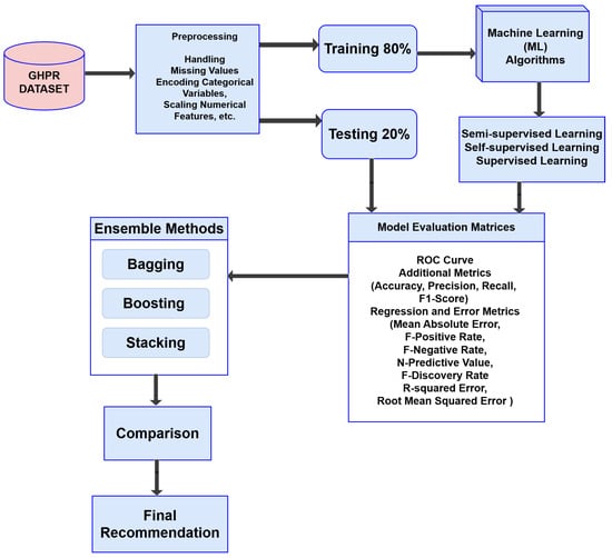
Figure 1.
Proposed methodology for finding software defects.
3.1. Dataset
This study utilized the GHPR imbalanced dataset from Kaggle [19]. The dataset comprises twenty-two features for analyzing software defects. Of these, twenty-one are independent features, while one is a dependent feature indicating the presence of software defects. The GHPR dataset contains a total of 2109 instances, with a class distribution of 326 instances featuring faults and 1783 instances without faults. In the dataset, a value of 1 represents a fault, while a value of 0 indicates no fault. Figure 2 illustrates the distribution of faults along with the corresponding values for the fault-free dataset.
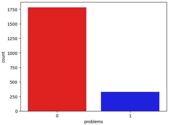
Figure 2.
Faulty and non-faulty data count.
3.2. Data Prepossessing
Data preparation and cleaning involve converting raw data into a format that is ready for analysis. This process includes addressing missing values, scaling numerical features, and encoding categorical variables. Here, we utilized Min–Max scaling to ensure that all variables are brought to a similar scale.
3.3. ML Algorithms
- Logistic Regression (LR): By using the data to fit a linear equation observed, the LR method establishes the relationship between independent and dependent features [20]. For LR, the activation function is explained as:Here, e = natural logarithm base and value = the number that one wants to change.Logistic Regression (LR)—Sigmoid Function (SF); Here, m denotes the value of input, n is the output that is predicted, is the term of intercept, and is the coefficient of the input value (m).
- Random Forest (RF): Multiple decision trees are built by the machine learning algorithm RF, which then aggregates the predictions by voting or averaging them [21].Here, is the ith decision tree’s prediction, N is the forest’s total tree count, and is the ensemble prediction.
- Decision Tree (DT): The DT algorithm partitions data based on features to predict outcomes. Its equation Z(m) is represented by recursive splitting, optimizing purity measures like Gini impurity or entropy [22]. The Gini impurity measure is given byHere, e represents the total number of classes, and shows the percentage of samples in class i in set m. The entropy measure is given bywith m having e classes, where the percentage of samples in class i is shown by .
- Gradient Boosting (GB): GB is an algorithm of machine learning that iteratively improves weak learners by minimizing a loss function. This algorithm is represented as an iterative process of combining weak learners (m) to minimize the overall loss function, typically through gradient descent. The function at each stage m in the gradient boosting algorithm is represented as m combines weak learners to approximate the true functions [23].
- Support Vector Machines (SVMs): SVM is the powerful supervised learning method for regression and classification in order to choose the best hyperplane for maximizing the class margin. The decision boundary in SVM is represented as, where represents weights, denotes input features, and b is the term of bias [24].
- K-Nearest Neighbors (KNN): The KNN algorithm classifies data items depending on the majority class of the k nearest neighbors. If a new data point m is given, the KNN classifier estimates the class label of k’s nearest neighbors by using the majority vote.Here, the number of features is n, and the ith training instance is . Choose the k locations with the shortest distances to determine the k nearest neighbors [22].
- AdaBoost Classifier (AC): The AC algorithm incorporates weak learners to create a powerful classifier by iterative adjusting weights. Its mathematical equation iswhere are the weights and are weak learners [25].
- Gaussian Classifier (GC): A GC is a common probabilistic model assuming features’ normal distribution, often applied to classification tasks with continuous features presumed to be independent given class labels [26].Let m be the feature of the vector and n be the label of the class. The Gaussian naive Bayes classifier determines the posterior probability using Bayes’ theorem:where = the posterior probability of class n given characteristics m, = the probability of seeing features m for class n, = class n’s prior probability, and = the probability of focusing on features m, also known as the evidence.
- Quadratic Discriminant Analysis (QDA): Assuming that every class has a multivariate normal distribution, the QDA classification algorithm calculates a unique covariance matrix for each class. Unlike Gaussian NB, QDA does not assume equal covariance matrices across classes [27]. In the case of class n and a feature vector m, the probability density function is as follows:where f is the feature number, is the class n mean vector, and is the class n covariance matrix. Assigning an input vector m to the class with the highest posterior probability is the decision rule for classifying it:
- Ridge Classifier: This is commonly used in scenarios where there’s multicollinearity among the features. The ridge classifier intends to minimize the goal function listed below:Here, the feature matrix is represented by M, the target vector by n, the coefficient vector by w, and the regularization parameter by [27].
4. Experimental Result and Analysis
During the analysis of the experimental results, we applied a number evaluation methods, including mean absolute error (MAE), R-squared error (RSE), root mean squared error (RMSE), false positive rate (F-Positive), false negative rate (F-Negative), negative predictive value (N-Predictive), false discovery rate (F Discovery Rate), recall, F1-score, precision, and accuracy.
4.1. Evaluation Metrics
This section explains the assessment metrics applied to evaluate the effectiveness of the machine learning algorithms created for the study. The chosen metrics offer an entire understanding of the predictive power of the model, its power to extrapolate the unknown data, and its overall performance.
ROC Curve and AUC: The ROC curve’s x-axis displays the FPR. FPR is misclassifying negative events as positive. The ROC curve’s y-axis shows the true positive rate (TPR), also known as recall or sensitivity. TPR is the number of correctly classified positives. An ideal classifier has a TPR of 1 and an FPR of 0. This value implies that the classifier would have identified all positive events but not any negative ones. The ROC curve places this point in the upper left corner. The classifier performs better as its ROC curve approaches the upper left corner. The ROC curve area measures classifier performance. Higher AUCs indicate better performance.
The ROC curve (Figure 3) lists the AUCs for several different machine learning models. The best-performing models according to this metric are quadratic discriminant analysis and GaussianNB, which both have an AUC of around 0.8.

Figure 3.
ROC curve for supervised learning.
In Figure 4, the bagged ensemble model with the highest AUC is the bagged ridge classifier, with an AUC of 0.8. The model also has the greatest TPR of all false-positive rates. The bagged decision tree, bagged AdaBoost classifier, bagged passive-aggressive classifier, bagged Gaussian naive Bayes (GaussianNB) algorithm, and bagged logistic regression models all exhibit similar AUCs, ranging from 0.74 to 0.79. In contrast, the bagged support vector classifier (SVC) and bagged K-nearest neighbors (KNN) models show lower AUCs at 0.65 and 0.72, respectively.
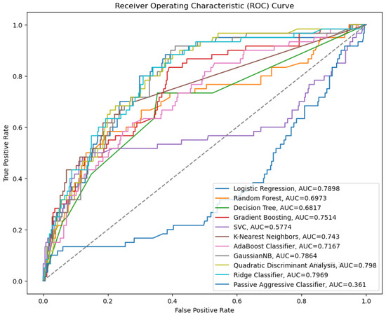
Figure 4.
ROC curves for bagged models.
Figure 5 demonstrates that the boosted logistic regression model achieves the highest AUC (area under the curve) of 0.79, indicating that, among all the models analyzed, it performs the best overall. Below is a summary of the models’ performance based on the AUC values: The boosted SVC, boosted AdaBoost classifier, and boosted random forest models all have comparable AUCs, ranging from 0.73 to 0.76. Boosted gradient boosting has an AUC of 0.68, while the boosted decision tree has the lowest AUC at 0.56.
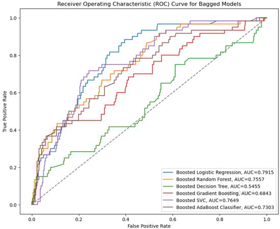
Figure 5.
ROC curves for boosted models.
Therefore, based on the AUC, the boosted logistic regression model performs best. The boosted decision tree model has the lowest AUC, indicating undesirable performance in the distinction between positive and negative cases. On the other hand, Figure 6 shows that the stacking AUC is 0.7996. The dashed line in the plot of the ROC curve indicates the performance of a random classifier. In this case, the stacking model achieved an AUC of 0.7996, which is notably higher than the random line. This suggests that the stacking model is performing effectively.
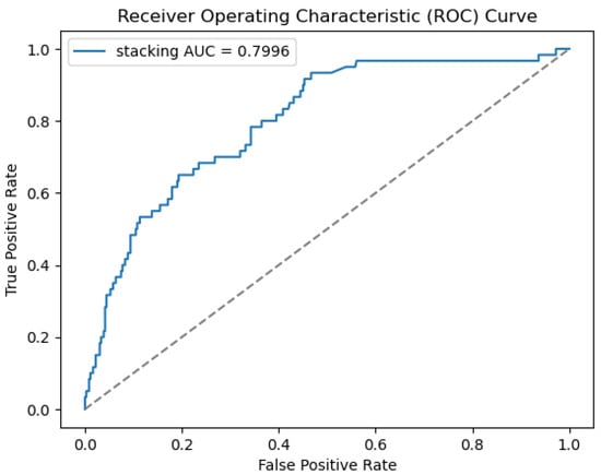
Figure 6.
ROC curves for stacking models.
- Additional Metrics:
- –
- Accuracy: It evaluates the model’s overall accuracy. In accuracy, the higher value is the better outcome.
- –
- Recall: It calculates the percentage of actual positives among all genuine positive predictions. Higher is better, especially in situations where missing positives costly.
- –
- Precision: Of all positive forecasts, it calculates the percentage of real positive predictions. Higher values are better, especially when false positives are unwanted or expensive.
- –
- F1-score: A balance between precision and recall is provided by the harmonic mean of the two. Since it shows a good balance between recall and precision, higher is preferable.
- Regression and Error Metrics:
- –
- False Positive Rate (F-Positive): This calculates the proportion of incorrectly negatives classified as positives. For F-Positive, lower is preferable.
- –
- False Negative Rate (F-Negative): This measures the proportion of positives incorrectly classified as negatives. Lower is better, as it means fewer actual positives are missed.
- –
- Negative Predictive Value (N-Predictive): This calculates the ratio of true negatives among all predicted negatives. Higher is better, as it indicates the model is accurately identifying negatives.
- –
- False Discovery Rate (F-Discovery Rate): This calculates the ratio of false positives among all predicted positives. Lower is better, as it means fewer incorrect predictions among the positive predictions.
- –
- Mean Absolute Error (MAE): This calculates the average amount of discrepancies between expected and actual values, without taking instructions. Lower is better, as it means the predictions are closer to the actual values.
- –
- R-squared Error (RSE): This calculates the standard deviation of residuals (prediction errors). It reflects the unexplained variance in the data. Lower is better, as it indicates the model fits the data more accurately with fewer errors.
- –
- Root Mean Squared Error (RMSE): It calculates the square root of average squared deviations between actual and expected values. Compared to MAE, it penalizes major mistakes more. Lower is better, as it means fewer prediction errors, particularly penalizing larger deviations.
4.2. Performance Analysis
This study used Python 3.13.1 code for performance investigation of datasets and implemented all ML algorithms.
The results are shown in Table 1; gradient boosting achieved the highest accuracy of 90.10%, closely followed by the AdaBoost classifier at 89.60%. These models also performed better in different evaluation metrics, showing that they are good at accurately identifying the target variable and distinguishing between different classes, especially since GB works well with imbalanced datasets. The result suggests that it is a reliable model for the GHPR dataset. Gaussian naive Bayes and quadratic discriminant analysis demonstrated lower performance compared to other models, suggesting they may not be the most suitable choices for this dataset.

Table 1.
Supervised learning classification report.
To validate the observed performance differences among classifiers, statistical significance testing was conducted. A 10-fold cross-validation was employed for each classifier to ensure stable evaluation. For key performance metrics—accuracy and F1-score—the mean values and their corresponding 95% confidence intervals (CI) were calculated. Additionally, a paired t-test was applied to compare each classifier’s performance with the best-performing model (gradient boosting). The null hypothesis assumed no significant performance difference between the compared models. A significance level of = 0.05 was used.
The results in Table 2 indicate that gradient boosting’s improvements in accuracy and F1-score are statistically significant compared to most other classifiers, with p-values < 0.05 in these comparisons. This confirms that the performance differences are not due to random variation but reflect genuine improvements.
Table 2.
Statistical significance testing and confidence intervals.
Table 3 presents an overview of the performance of each semi-supervised algorithm in terms of accuracy, recall, precision, F1-score, and other metrics. GAN stands out as the top performer across most metrics, including accuracy, F1-score, recall, MAE, RSE, and RMSE. It excels at balancing precision and recall, making it particularly effective for semi-supervised learning. S3VM also performs well across all metrics but falls slightly short of GAN, especially regarding F1-score, recall, and RSE. The autoencoder shows strong performance in specificity, achieving a perfect score in that metric; however, it underperforms in most other areas, particularly in F1-score and recall. In summary, GAN is the best-performing model in this comparison, with S3VM as a solid alternative, and the autoencoder lagging behind in overall performance.
Table 3.
Semi-supervised classification report.
Table 4 offers insights into the efficiency of each self-supervised algorithm, assessing metrics such as accuracy, recall, precision, and F1 score. Overall, SimCLR outperforms the other algorithms in terms of these metrics. BYOL shows slightly lower performance than SimCLR in most categories, yet it remains comparable regarding predictive ability, F1 score, and recall. Ultimately, SimCLR is the leading performer, with BYOL closely following, while the autoencoder ranks last based on these evaluation criteria.
Table 4.
Self-supervised classification report.
Using the confusion matrix (GB) study, we analyzed the result based on the number of true positive values (1186) true negative values (714), false positive values (63), and false negative values (146) (Figure 7). Based on the findings, the study determines the level of accuracy based on the mathematical formula (TP + TN)/(TP + TN + FP + FN). The study provides the overall accuracy of the model, which is the percentage of total samples correctly classified by the classifier.
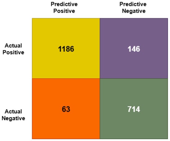
Figure 7.
Confusion metrics of GB model.
5. Conclusions
This study analyzes machine learning (ML) algorithms and finds the best software features for defect resolution that stakeholders, analysts, and software engineers can use. Identifying software defects’ root causes ensures quality, reliable, and maintainable software. We fixed missing values, standardized numerical data to a similar range, and Min–Max scaled categorical data before training and testing the model. We used a generic randomization process to balance labeled (50%) and unlabeled (50%) data for semi-supervised learning models. The study used twenty-two characteristics to make predictions.
Gradient boosting and AdaBoost classifier performed best for the GHPR dataset after a thorough evaluation using multiple performance metrics. This process encoded categorical variables, corrected missing values, and uniformly scaled numerical features using Min–Max scaling. Ensemble methods improved prediction accuracy over individual models. One limitation of this study is the exclusive use of the GHPR dataset for model training and evaluation. Although the GHPR dataset is useful and contains extensive information about defects relevant to achieving study goals, it may not adequately represent the diversity of software engineering projects across various fields. As a result, the generalizability of our findings to other datasets or industrial settings may be limited.
The plan is to extend future evaluation to include additional benchmark datasets such as those from the PROMISE repository, particularly the NASA MDP dataset. This will allow the assessment of the robustness and adaptability of the proposed models across different types of software projects and development environments. Moreover, future studies may explore domain adaptation techniques to enhance model transferability between heterogeneous datasets.
Author Contributions
Conceptualization, A.S.; Validation, M.B.; Formal analysis, A.S. and F.A.F.; Investigation, A.S. and M.B.; Resources, A.S.; Data curation, A.S.; Writing—original draft, A.S. and F.A.F.; Writing—review and editing, M.B., J.U., and H.A.K.; Visualization, A.S.; Supervision, M.B.; Project administration, H.A.K.; Funding acquisition, H.A.K. All authors have read and agreed to the published version of the manuscript.
Funding
This research was funded by Multimedia University, Cyberjaya, Selangor, Malaysia (Grant Number: PostDoc (MMUI/240029)).
Institutional Review Board Statement
Not applicable.
Informed Consent Statement
Not applicable.
Data Availability Statement
https://github.com/JiaUddinPhD/Seminar-on-Tabular-data-and-XAI/blob/main/dataset.csv (accessed on 10 July 2025).
Conflicts of Interest
The authors declare no conflicts of interest.
References
- Fan, C.; Lei, Y.; Sun, Y.; Mo, L. Novel transformer-based self-supervised learning methods for improved HVAC fault diagnosis performance with limited labeled data. Energy 2023, 278, 127972. [Google Scholar] [CrossRef]
- Petrovic, A.; Jovanovic, L.; Bacanin, N.; Antonijevic, M.; Savanovic, N.; Zivkovic, M.; Gajic, V. Exploring metaheuristic optimized machine learning for software defect detection on natural language and classical datasets. Mathematics 2024, 12, 2918. [Google Scholar] [CrossRef]
- Ramírez-Sanz, J.M.; Maestro-Prieto, J.A.; Arnaiz-González, Á.; Bustillo, A. Semi-supervised learning for industrial fault detection and diagnosis: A systemic review. ISA Trans. 2023, 143, 255–270. [Google Scholar] [CrossRef] [PubMed]
- Albayati, M.G.; Faraj, J.; Thompson, A.; Patil, P.; Gorthala, R.; Rajasekaran, S. Semi-supervised machine learning for fault detection and diagnosis of a rooftop unit. Big Data Min. Anal. 2023, 6, 170–184. [Google Scholar] [CrossRef]
- De Vries, S.; Thierens, D. A reliable ensemble-based approach to semi-supervised learning. Knowl.-Based Syst. 2021, 215, 106738. [Google Scholar] [CrossRef]
- Askari, B.; Cavone, G.; Carli, R.; Grall, A.; Dotoli, M. A semi-supervised learning approach for fault detection and diagnosis in complex mechanical systems. In Proceedings of the 2023 IEEE 19th International Conference on Automation Science and Engineering (CASE), Auckland, New Zealand, 26–30 August 2023; pp. 1–6. [Google Scholar] [CrossRef]
- Wang, H.; Liu, Z.; Ge, Y.; Peng, D. Self-supervised signal representation learning for machinery fault diagnosis under limited annotation data. Knowl.-Based Syst. 2022, 239, 107978. [Google Scholar] [CrossRef]
- Wang, X.; Kihara, D.; Luo, J.; Qi, G.-J. Enaet: A self-trained framework for semi-supervised and supervised learning with ensemble transformations. IEEE Trans. Image Process. 2021, 30, 1639–1647. [Google Scholar] [CrossRef]
- Mehmood, I.; Shahid, S.; Hussain, H.; Khan, I.; Ahmad, S.; Rahman, S.; Ullah, N.; Huda, S. A novel approach to improve software defect prediction accuracy using machine learning. IEEE Access 2023, 11, 63579–63597. [Google Scholar] [CrossRef]
- Md Rashedul Islam, M.B.; Akhtar, M.N. Recursive approach for multiple step- ahead software fault prediction through long short-term memory (LSTM). J. Discret. Math. Sci. Cryptogr. 2022, 25, 2129–2138. [Google Scholar] [CrossRef]
- Han, T.; Xie, W.; Pei, Z. Semi-supervised adversarial discriminative learning approach for intelligent fault diagnosis of wind turbine. Inf. Sci. 2023, 648, 119496. [Google Scholar] [CrossRef]
- Qi, G.-J.; Luo, J. Small data challenges in big data era: A survey of recent progress on unsupervised and semi-supervised methods. IEEE Trans. Pattern Anal. Mach. Intell. 2022, 44, 2168–2187. [Google Scholar] [CrossRef] [PubMed]
- Šikić, L.; Afrić, P.; Kurdija, A.S.; Šilić, M. Improving software defect prediction by aggregated change metrics. IEEE Access 2021, 9, 19391–19411. [Google Scholar] [CrossRef]
- Meng, A.; Cheng, W.; Wang, J. An integrated semi-supervised software defect prediction model. J. Internet Technol. 2023, 24, 1307–1317. [Google Scholar] [CrossRef]
- Begum, M.; Rony, J.H.; Islam, M.R.; Uddin, J. A long-term software fault prediction model using box-cox and linear regression. J. Inf. Syst. Telecommun. 2023, 11, 222–233. [Google Scholar]
- ul Haq, Q.M.; Arif, F.; Aurangzeb, K.; ul Ain, N.; Khan, J.A.; Rubab, S.; Anwar, M.S. Identification of software bugs by analyzing natural language-based requirements using optimized deep learning features. Comput. Mater. Contin. 2024, 78, 4379–4397. [Google Scholar]
- Villoth, J.P.; Zivkovic, M.; Zivkovic, T.; Abdel-salam, M.; Hammad, M.; Jovanovic, L.; Bacanin, N. Two-tier deep and machine learning approach optimized by adaptive multi-population firefly algorithm for software defects prediction. Neurocomputing 2025, 630, 129695. [Google Scholar] [CrossRef]
- Begum, M.; Shuvo, M.H.; Ashraf, I.; Mamun, A.A.; Uddin, J.; Samad, M.A. Software defects identification: Results using machine learning and explainable artificial intelligence techniques. IEEE Access 2023, 11, 132750–132765. [Google Scholar] [CrossRef]
- Rahman, S. Soft Defect Dataset. Kaggle. 2019. Available online: https://www.kaggle.com/datasets/sazid28/soft-defect/data (accessed on 10 July 2025).
- Tapu Rayhan, M.H.N.S. Ayesha Siddika: Social media emotion detection and analysis system using cutting-edge artificial intelligence techniques. In Proceedings of the 9th International Congress on Information and Communication Technology (ICICT 2024), London, UK, 19–22 February 2024. [Google Scholar]
- Breiman, L. Random forests. Mach. Learn. 2001, 45, 5–32. [Google Scholar] [CrossRef]
- Cover, T.; Hart, P. Nearest neighbor pattern classification. IEEE Trans. Inf. Theory 1967, 13, 21–27. [Google Scholar] [CrossRef]
- Friedman, J.H. Greedy function approximation: A gradient boosting machine. Ann. Stat. 2001, 29, 1189–1232. [Google Scholar] [CrossRef]
- Cortes, C.; Vapnik, V. Support-vector networks. Mach. Learn. 1995, 20, 273–297. [Google Scholar] [CrossRef]
- Freund, Y.; Schapire, R.E. A decision-theoretic generalization of on-line learning and an application to boosting. J. Comput. Syst. Sci. 1997, 55, 119–139. [Google Scholar] [CrossRef]
- Bishop, C.M. Pattern Recognition and Machine Learning; Springer: New York, NY, USA, 2006. [Google Scholar]
- Hastie, T.; Tibshirani, R.; Friedman, J. The Elements of Statistical Learning: Data Mining, Inference, and Prediction; Springer: New York, NY, USA, 2009. [Google Scholar]
Disclaimer/Publisher’s Note: The statements, opinions and data contained in all publications are solely those of the individual author(s) and contributor(s) and not of MDPI and/or the editor(s). MDPI and/or the editor(s) disclaim responsibility for any injury to people or property resulting from any ideas, methods, instructions or products referred to in the content. |
© 2025 by the authors. Licensee MDPI, Basel, Switzerland. This article is an open access article distributed under the terms and conditions of the Creative Commons Attribution (CC BY) license (https://creativecommons.org/licenses/by/4.0/).