Raman Spectra Classification of Pharmaceutical Compounds: A Benchmark of Machine Learning Models with SHAP-Based Explainability

Abstract

Raman spectroscopy has become an indispensable analytical technique in pharmaceutical research, offering non-invasive, rapid, and chemically specific insights into pharmaceutical compounds. In this study, we present a comprehensive benchmark of machine learning models for classifying 32 pharmaceutical compounds based on their Raman spectral signatures. A diverse array of algorithms—including Support Vector Machines (SVMs), Random Forests, k-Nearest Neighbors (k-NN), Gradient Boosting (XGBoost, LightGBM), and 1D Convolutional Neural Networks (CNNs)—were evaluated on a publicly available dataset. The results demonstrate outstanding classification performance across models, with linear SVM achieving the highest accuracy of 99.88%, followed closely by CNN (99.26%). Ensemble methods such as Random Forest and XGBoost also yielded high accuracies above 98.3%. In addition to strong predictive performance, SHAP (SHapley Additive exPlanations) analysis was employed to interpret model decisions. CNN models, in particular, revealed well-localized and chemically meaningful spectral regions critical to classification. This combination of high accuracy and interpretability highlights the promise of explainable AI in pharmaceutical analysis and quality control, offering robust, transparent, and scalable solutions for real-world applications.

1. Introduction

Raman spectroscopy is extensively utilized in pharmaceutical analysis, enabling precise identification of chemical compounds, quality control, and the development of Active Pharmaceutical Ingredients (APIs). Recent advances in Raman-based analytics have significantly expanded their role in pharmaceutical applications.

Recent advances and emerging trends in Raman spectroscopy are significantly reshaping pharmaceutical analysis and quality control, particularly through their impact on real-time and on-site applications. Raman spectroscopy is being increasingly recognized by regulatory bodies such as the European and US Pharmacopoeias as a valid analytical process. However, it still lacks specific inclusion in individual substance monographs, which has limited its broader clinical adoption [1]. Raman spectroscopy offers several advantages, including non-destructive and label-free analysis, compatibility with various physical states (solids, liquids, gases), and minimal sample preparation. These features make it a powerful tool for detecting counterfeit drugs, supporting the development of personalized medicines, and enabling continuous pharmaceutical manufacturing processes.

Spontaneous Raman spectroscopy is effective for the identification of raw material and the monitoring of physical forms such as polymorphs [2]. UV and deep-UV Raman techniques enhance sensitivity to specific molecular vibrations, making them suitable for biological macromolecule analysis [3]. Surface-enhanced Raman spectroscopy (SERS) increases signal intensity by using metallic nanostructures, thus enabling the detection of trace analytes [4]. Coherent Raman methods like CARS and SRS allow for rapid, label-free molecular imaging, useful for in vivo studies and understanding drug distribution [5].

Technological innovations have significantly expanded the capabilities of Raman spectroscopy. Raman microscopes now facilitate hyperspectral 3D imaging. Immersion fiber optic probes facilitate in-line monitoring during manufacturing. Handheld devices are increasingly being used for field analysis and verification of raw materials. Spatial Offset Raman Spectroscopy (SORS) enables analysis through opaque packaging, while Fiber-Enhanced Raman Spectroscopy (FERS) allows for sensitive detection of compounds in gases and liquids [6]. Machine learning and chemometric techniques enable classification and quantitative analysis of complex datasets. User-friendly software tools such as RAMANMETRIX help non-expert users perform sophisticated spectral analyses. However, the standardization and reproducibility of data processing workflows remain challenges for broader industrial and clinical adoption [7]. Also, Raman spectroscopy has been used for the quality control of 3D-printed medications, virus detection via SERS-based microdevices, and monitoring of drug resistance in pathogens [8].

Raman spectroscopy has become a versatile analytical tool in pharmaceutical science, with techniques such as dispersive Raman, FT-Raman, SERS, and resonance Raman being widely applied for quality control, counterfeit detection, and drug formulation analysis [9,10]. Recent advances have demonstrated the integration of Raman data with machine learning (ML) and deep learning (DL) methods to enhance classification, quantification, and process monitoring tasks. For example, deep learning-based SERS strategies have been used for identifying protein binding sites [11], while CNNs have been employed for real-time quality control in tablet manufacturing [12].

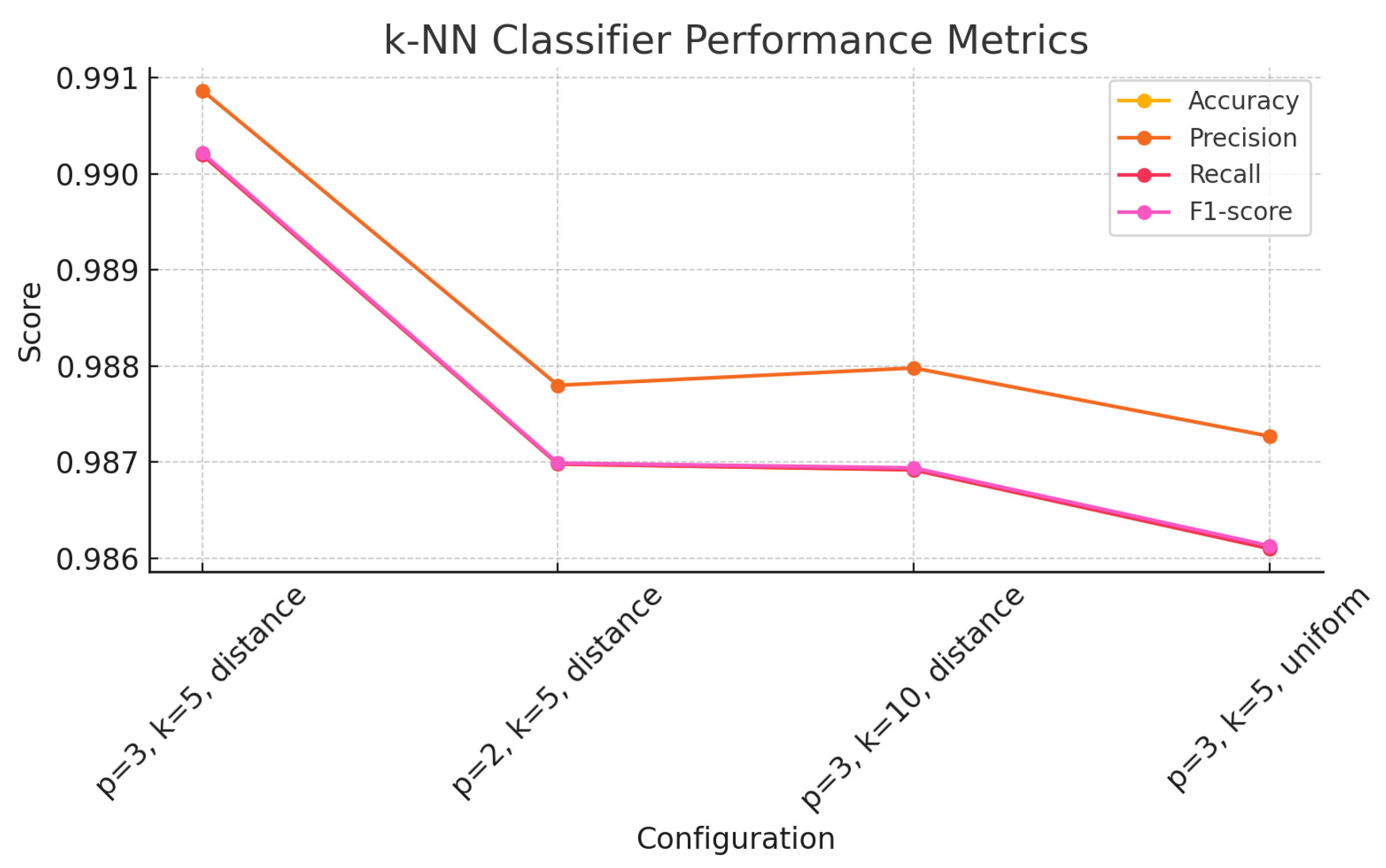
Several studies have demonstrated the efficacy of ML algorithms—including SVMs, Random Forest, XGBoost, and artificial neural networks—for spectral classification and drug dissolution prediction [13,14,15]. Additionally, applications range from particle identification in injectable drug production [16] to the detection of drug residues on latent fingermarks [17]. ML-enhanced Raman spectroscopy has also proven effective for colonic drug delivery optimization [18], falsified medicine detection [19], and CHO cell culture monitoring [20]. Furthermore, collaborative platforms have enabled large-scale model development for monoclonal antibody quantification [21]. These works collectively underscore the increasing synergy between Raman spectroscopy and ML in advancing pharmaceutical research and quality assurance.

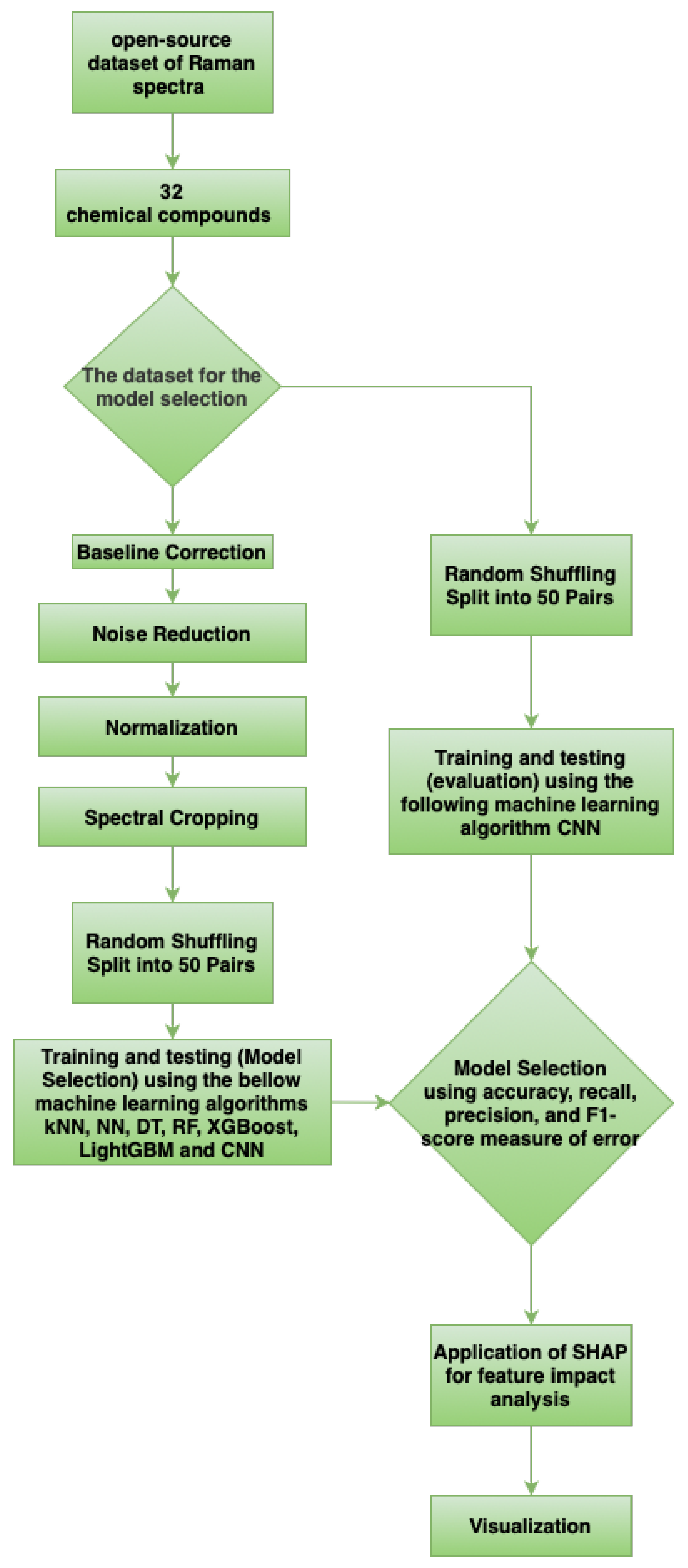
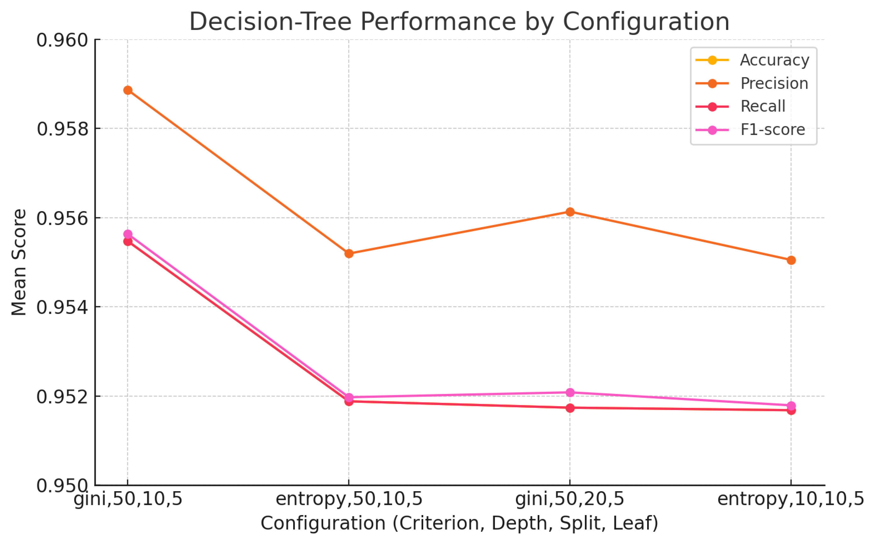
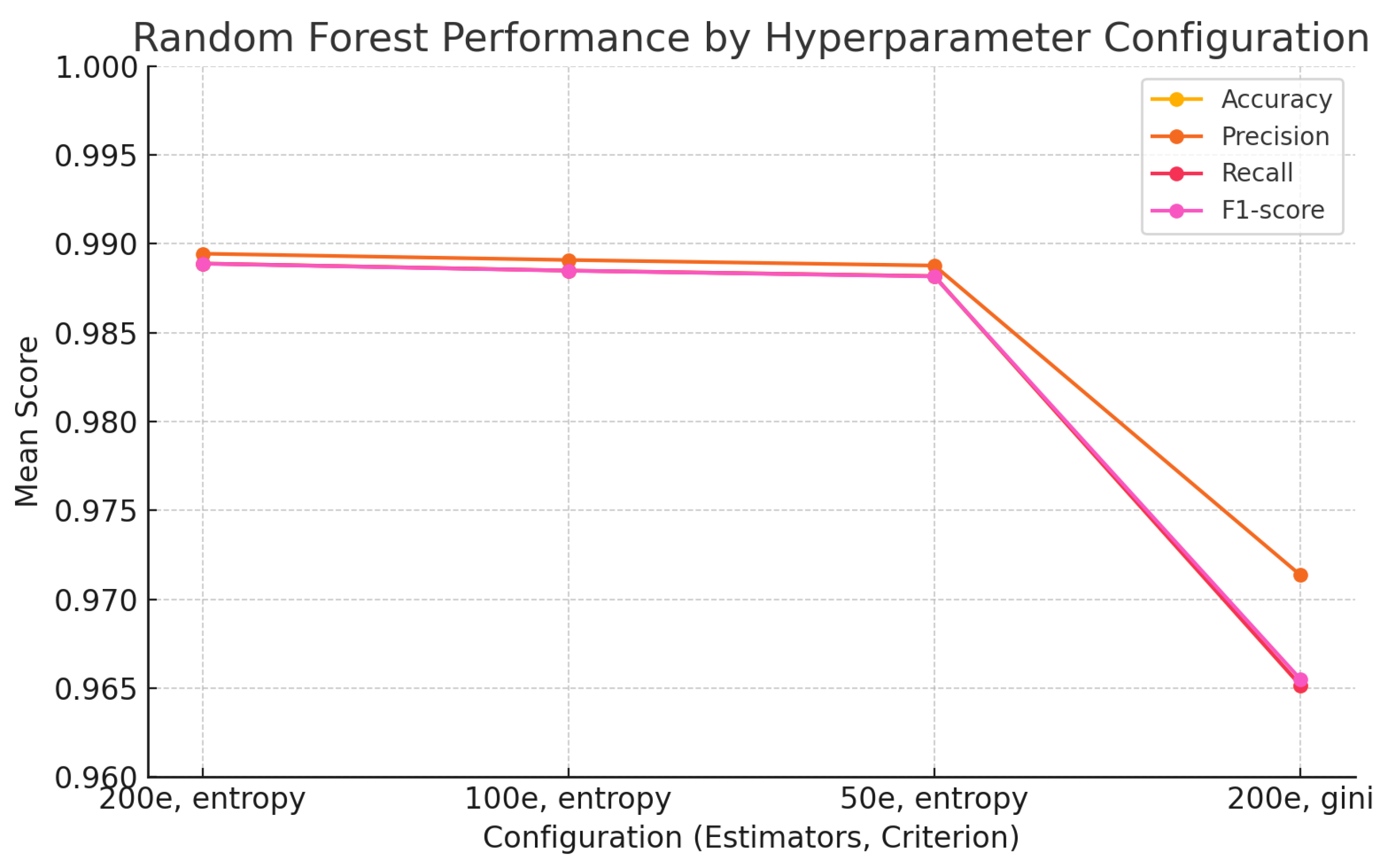
In this study, we present a systematic comparison of multiple machine learning algorithms for the classification of pharmaceutical compounds based on Raman spectral data. The evaluated models include both traditional approaches—such as Support Vector Machines (SVMs), Random Forests, and k-Nearest Neighbors (k-NN)—as well as a deep learning architecture in the form of a one-dimensional Convolutional Neural Network (1D CNN). In addition to assessing classification performance, we incorporate SHAP-based explainability techniques to interpret the decision-making process of the models. This integration not only enhances transparency but also offers deeper chemical insight into the spectral regions that are most influential for compound differentiation.

2. Methods and Materials

2.1. Dataset and Data Acquisition

The study published by Flanagan et al. [22] introduces an open-source dataset of Raman spectra for 32 chemical compounds frequently used in API manufacturing. This dataset includes a total of 3510 samples with spectral data spanning the range of 150 to 3425 cm⁻¹, capturing key vibrational modes essential for chemical identification and analysis (

Table 1. List of 32 pharmaceutical compounds with assay, exposure time, pixel fill, and sample count.

Name	Assay	Exposure	Pixel Fill	Samples
1,3-Dimethyl-2-imidazolidinone	≥99.0	3	50	109
2-Propanol	≥99.8	5	50	109
2,2-Dimethoxypropane	≥98.0	5	60	107
4-Methyl-2-pentanone	≥99.5	15	50	100
Acetic acid glacial	≥99.8	7.5	60	113
Acetone	≥99.8	7	73	120
Acetonitrile	≥99.9	10	50	104
Benzaldehyde	≥99.0	2	68	121
Benzyl bromide	≥98.0	2	73	112
Butyl acetate	≥99.7	20	51	106
Chloroform	≥99.8	2	70	122
Cyclohexane	≥99.8	2	70	145
Dichloromethane	≥99.5	5	55	111
Diethyl malonate	≥99.0	30	63	100
Diethylamine	≥99.0	15	60	107
Diethylene glycol	≥99.0	30	50	105
Dimethyl sulfoxide	≥99.8	2	60	105
Ethanol	≥99.9	10	56	109
Ethyl acetate	≥99.8	10	50	110
Ethylene glycol	≥99.0	15	70	101
Formic acid	≥98.0	20	55	110
Isobutylamine	≥99.0	20	60	104
Methanol	≥99.8	15	50	101
Methyl isobutyl ketone	≥99.5	20	55	105
N,N-Dimethylformamide	≥99.8	10	40	105
n-Heptane	≥95.0	45	68	103
n-Hexane	≥98.0	30	55	102
Propyl acetate	≥99.0	20	63	107
tert-Butanol	≥99.7	3	51	113
tert-Butyl methyl ether	≥99.8	3	60	117
Tetrahydrofuran	≥99.9	5	70	100
Toluene	≥99.9	2	67	127

). The experimental setup described in the study involves an Endress+Hauser Raman Rxn2 analyzer, operating with a 785 nm laser for excitation and a spectral resolution of 1 cm⁻¹. The spectra were collected using an Rxn-10 probe and stored as CSV files for reproducibility and open access. The dataset covers solvents and reagents with purities exceeding 98%, ensuring high-quality reference data for machine learning applications. Also, Flanagan et al. [22] included detailed quality control protocols to ensure spectral integrity, reproducibility, and chemical validity. The data acquisition process involved the following:

• Wavelength calibration was performed daily following a 120-min system warm-up and automatic calibration routine, in accordance with the manufacturer’s guidelines. Intensity calibration was carried out using a certified cyclohexane standard.
• Signal optimization through 50–70% pixel fill targeting to prevent detector saturation.
• Automated preprocessing, including dark noise subtraction, cosmic ray filtering, and intensity correction, was performed via the iC Raman software version 4.1 during acquisition.
• Validation of reproducibility, where the most intense fingerprint-region peaks were monitored across multiple replicates per compound. Reported standard deviations of peak maxima were consistently below 1 cm⁻¹ for most substances, confirming high spectral stability (see [22]; Figure 2).

Furthermore, the dataset includes curated Raman band assignments for each compound (Tables 2 and 3 in [22]), ensuring accurate chemical identification. These quality control measures provide a robust foundation for machine learning analysis without the need for additional spectral validation.

2.2. Methodology Workflow

The proposed workflow ensures a comprehensive approach, combining robust preprocessing, diverse model comparison, and explainability analysis to yield reliable and interpretable results in Raman spectra classification.

The diagram in Figure 1 illustrates the experimental workflow used for the classification of pharmaceutical compounds based on Raman spectral data. The methodology is structured into clearly defined stages, from dataset preparation to model evaluation and explainability analysis. Below is a step-by-step breakdown:

• Data Acquisition: The process begins with an open-source Raman spectral dataset comprising 32 distinct chemical compounds.
• Preprocessing: A series of preprocessing steps are applied to the spectral data to enhance model performance:
• Spectral Cropping: In our analysis, the only additional preprocessing step we applied was spectral cropping, restricting the input range to 150–1150 cm⁻¹ (see Figure 2). This region corresponds to the fingerprint range of the Raman spectrum, where most structurally and chemically informative vibrational modes of small organic molecules are located. Cropping to this range achieves the following:

  (a)

  It excludes high-wavenumber regions (>1150 cm⁻¹) that often contain redundant or low-signal information for this classification task;

  (b)

  It reduces data dimensionality and training time;

  (c)

  It focuses model learning on discriminative spectral features such as C–C stretching, C–O bending, and aromatic ring deformations.

  This focused preprocessing strategy was chosen to enhance both model performance and chemical interpretability.
• Data Splitting: The cleaned dataset is randomly shuffled and split into 50 pairs for training and evaluation purposes.
• Model Evaluation (CNN): A 1D Convolutional Neural Network (CNN) is trained and tested directly on the preprocessed dataset to establish baseline performance.
• Model Selection: Multiple machine learning algorithms—including k-Nearest Neighbors (kNN), Neural Networks (NNs), Decision Trees (DTs), Random Forests (RFs), XGBoost, LightGBM, and CNN—are trained and evaluated. Models are assessed based on accuracy, precision, recall, and F1-score.
• Explainability (SHAP): SHAP (SHapley Additive exPlanations) values are calculated to interpret the model’s predictions and identify which spectral features contributed most significantly to classification decisions.
• Visualization: The final step involves visualizing the SHAP results and performance metrics to communicate findings effectively.

All code used for data preprocessing, model training, and SHAP-based interpretation is available in a public GitHub repository: https://github.com/Lorvec/Raman-Spectra-Classification-of-Pharmaceutical-Compounds, accessed on 20 June 2025. The repository includes a Jupyter Notebook with step-by-step documentation, allowing for full reproduction of the results presented in this study.

2.3. Machine Learning Models

To ensure a systematic and meaningful comparison, we organized the candidate models into methodological families, including distance-based algorithms (e.g., k-NN), ensemble tree-based models (e.g., Random Forest, XGBoost, LightGBM), and deep learning architectures (e.g., CNN). Within each family, we initially tested multiple algorithms and selected the top-performing models based on preliminary cross-validation results. This allowed us to identify the best representative from each group. In the final evaluation phase, we compared these selected models across families to assess their relative performance in classifying Raman spectral data. This hierarchical approach enabled us to capture the strengths of diverse algorithmic strategies while maintaining clarity and reproducibility in the comparison framework.

2.3.1. Decision Trees

Decision Trees are hierarchical models that split the data based on feature values, creating branches that represent decisions and outcomes. In the context of Raman spectra, Decision Trees can effectively identify key spectral features and create clear decision boundaries that represent chemical classes. Their interpretability makes them an ideal baseline for understanding the impact of different Raman shifts on classification accuracy. However, they are prone to overfitting, especially with high-dimensional spectral data, if not properly pruned [23].

2.3.2. Random Forests

Random Forests are an ensemble learning method that constructs multiple decision trees during training and aggregates their outputs for more robust predictions. Each tree is trained on a random subset of the data, which reduces variance and enhances generalization. This method is particularly effective for handling the multi-modal distributions typical of Raman spectra from complex chemical mixtures. Random Forests also provide insights into feature importance, enabling better understanding of influential Raman shifts [24].

2.3.3. k-Nearest Neighbors (k-NN)

The k-NN algorithm is a non-parametric method that classifies samples based on the proximity to their neighbors in the spectral space. For Raman spectra, k-NN excels in detecting local patterns and similarities between chemical signatures. Its simplicity and lack of assumption about the data distribution make it a flexible choice for spectral analysis, though its performance can degrade with high-dimensional data if not well normalized [24].

2.3.4. LightGBM

LightGBM is a gradient boosting framework that optimizes decision trees for fast training and low memory usage. It constructs trees leaf-wise, leading to more efficient utilization of high-dimensional Raman spectral data. LightGBM is particularly effective in modeling intricate spectral variations and identifying subtle differences in chemical signatures. It also supports automated handling of missing values, making it robust for real-world datasets.

2.3.5. XGBoost

XGBoost is an advanced gradient boosting method known for its scalability and high predictive performance. It employs second-order optimization techniques and regularization to minimize overfitting, which is crucial for the complexity of Raman spectra. XGBoost’s parallel processing capabilities allow it to be trained rapidly, making it ideal for large spectral datasets where speed and accuracy are critical [25].

2.3.6. Convolutional Neural Networks (CNNs)

A 1D Convolutional Neural Network (CNN) was implemented to automatically extract spatially coherent patterns from the Raman spectra. The architecture consisted of three convolutional layers: the first applied 10 filters of size 10, followed by two layers with 25 filters each. All layers used ReLU activations, batch normalization ($ϵ$ = $2\times {10}^{-5}$, momentum = 0.9), and dropout (rate = 0.25). An average pooling layer with a pool size of 8 reduced dimensionality before a fully connected softmax layer performed classification [26]. The network was trained using the Adam optimizer with a learning rate of 0.001 for 30 epochs and a batch size of 32. L2 regularization ($\lambda$ = $1\times {10}^{-4}$) was applied to all learnable layers. Raw, high-dimensional spectra were provided directly to the network, allowing it to learn complex local patterns without the need for explicit feature engineering. This design proved effective in modeling subtle shifts and peak patterns characteristic of Raman data.

2.4. Explainability of Machine Learning Models

To enhance model interpretability, Shapley Additive Explanations (SHAP) were applied across all models to identify the most influential spectral regions contributing to the classification outcomes [27]. Among all the models, the Convolutional Neural Network (CNN) demonstrated the highest predictive performance, effectively capturing complex spectral patterns directly from raw Raman data. A focused SHAP analysis on the CNN model revealed distinct high-intensity peaks that correspond to characteristic vibrational modes of key chemical compounds, as described in the reference dataset. These vibrational modes represent critical Raman bands that the CNN prioritized for accurate classification. The SHAP visualizations provided insight into how the CNN weighted these spectral features during decision-making. This interpretability analysis emphasizes the model’s capacity to automatically detect meaningful chemical signatures from raw spectra, supporting both identification and quality assessment of Active Pharmaceutical Ingredients (APIs).

3. Results

3.1. XGBoost Hyperparameter Comparison

Table 2. XGBoost performance for different, (n_ estimators, max_depth) settings.

Configuration	Accuracy	Precision	Recall	F1-Score
500e, 5d	0.98319	0.98440	0.98319	0.98327
500e, 10d	0.98319	0.98439	0.98319	0.98326
300e, 10d	0.98279	0.98402	0.98279	0.98286
300e, 5d	0.98265	0.98388	0.98265	0.98273

and Figure 3 summarize the performance of four XGBoost configurations, all with $\lambda =5$ and learning rate $=0.1$, varying only the number of estimators and maximum tree depth. Both the 500-estimator models ($\lambda =5$ and 10) achieve the highest accuracy and recall (0.98319), as well as the top F1-scores, while precision remains essentially unchanged between them. Reducing the ensemble to 300 trees yields a slight decline across all metrics, and further decreasing depth to 5 causes a marginal additional drop. Notably, increasing depth from 5 to 10 at 500 estimators produces no measurable improvement, indicating that a 500-tree forest of depth 5 is sufficient to capture the underlying structure of this dataset.

3.2. LightGBM Hyperparameter Comparison

Table 3. LightGBM performance for different (n_estimators, learning_rate, max _depth) settings.

Configuration	Accuracy	Precision	Recall	F1-Score
300e, lr = 0.1, 5d	0.98396	0.98497	0.98396	0.983998
300e, lr = 0.05, 5d	0.98376	0.98496	0.98376	0.983845
100e, lr = 0.1, 10d	0.98348	0.98445	0.98348	0.983505
300e, lr = 0.05, 10d	0.98333	0.98439	0.98333	0.983377

and Figure 4 report the performance of four LightGBM configurations, each using 50 leaves and varying the number of estimators, learning rate, and maximum tree depth. The best overall accuracy (0.98396) and recall (0.98396) are achieved by the model with 300 estimators, a learning rate of 0.1, and a max depth of 5, and this model also attains the highest F1-score. Reducing the learning rate to 0.05 at the same tree settings yields a marginal decrease in all metrics. A shallow forest with only 100 estimators and deeper trees (depth 10) results in slightly lower performance, and maintaining 300 estimators with depth 10 but with a low learning rate further diminishes the scores. These results indicate that, for this dataset, a forest of 300 trees at depth 5 and a learning rate of 0.1 offers the optimal trade-off between model complexity and predictive accuracy.

3.3. SVM Hyperparameter Comparison

Table 4. SVM performance for different (kernel, C) settings.

Configuration	Accuracy	Precision	Recall	F1-Score
linear, $C=0.1$	0.99880	0.99888	0.99880	0.99880
linear, $C=1.0$	0.99880	0.99888	0.99880	0.99880
rbf, $C=10.0$	0.94692	0.96856	0.94692	0.94881
rbf, $C=1.0$	0.90618	0.95134	0.90618	0.91432

and Figure 5 illustrate the mean accuracy, precision, recall and F1-score for four SVM configurations, varying the kernel (linear vs. RBF) and the regularization parameter C. When using a linear kernel ($C=0.1$ or $C=1.0$), the classifier achieves nearly perfect performance across all metrics (accuracy 0.9988). Switching to the RBF kernel results in a notable drop: with $C=10$, accuracy and recall fall to 0.9469, while precision remains relatively high at 0.9686; reducing C further to 1.0 under RBF yields an accuracy of 0.9062 and recall of 0.9062, with a corresponding F1-score of 0.9143. These trends highlight that the linear kernel robustly separates our two classes, whereas the RBF kernel’s performance heavily depends on C, trading off recall for precision as C increases.

3.4. k-NN Hyperparameter Comparison

The comparison in Figure 6 and

Table 5. k-Nearest Neighbors performance for different $(p,k,\mathrm{weights})$ settings.

Configuration	Accuracy	Precision	Recall	F1-Score
$p=3,k=5,$ distance	0.99020	0.99087	0.99020	0.99022
$p=2,k=5,$ distance	0.98698	0.98780	0.98698	0.98699
$p=3,k=10,$ distance	0.98692	0.98798	0.98692	0.98694
$p=3,k=5,$ uniform	0.98610	0.98727	0.98610	0.98613

shows that all four k-NN configurations deliver excellent classification performance, with accuracy, precision, recall and F1-score exceeding 98.6 %. The distance-weighted model with $p=3$ and $k=5$ attains the highest overall accuracy (99.02 %), and its precision and recall are essentially identical, yielding an F1-score of 99.02 %. When the neighborhood size is increased to $k=10$ (keeping $p=3$ and distance weighting), all metrics drop slightly but remain above 98.6 %. Reducing the Minkowski norm to $p=2$ (with $k=5$ and distance weighting) also causes a modest decline across the board. Finally, switching to uniform weighting (with $p=3$ and $k=5$) yields the lowest—but still very strong—performance, demonstrating that k-NN is robust to these parameter changes. Overall, the results underscore that small, distance-weighted neighborhoods best capture local spectral similarity for this classification task.

In Table 5, the K-Nearest Neighbors models are compared across four configurations differing in the distance norm p, number of neighbors k, and weighting scheme. The highest overall accuracy and recall (0.99020) are achieved by the model with $p=3$, $k=5$, and distance weights, which also attains the top F1-score (0.99022). Reducing the norm to $p=2$ or increasing k to 10 slightly decreases performance, while switching to uniform weights under the same p and k yields the lowest accuracy (0.98610) but maintains a strong F1-score (0.98613). This demonstrates that both the choice of distance metric and weighting method play significant roles in balancing precision and recall in K-NN classification.

3.5. Decision-Tree Hyperparameter Comparison

A comparative evaluation of four Decision Tree configurations (Figure 7 and

Table 6. Decision Tree performance for different configurations of splitting criterion, tree depth, and sample thresholds.

Configuration	Accuracy	Precision	Recall	F1-Score
gini, depth = 50, split = 10, leaf = 5	0.95547	0.95886	0.95547	0.95563
entropy, depth = 50, split = 10, leaf = 5	0.95188	0.95519	0.95188	0.95197
gini, depth = 50, split = 20, leaf = 5	0.95174	0.95613	0.95174	0.95208
entropy, depth = 10, split = 10, leaf = 5	0.95168	0.95505	0.95168	0.95179

) reveals that splitting criterion, tree depth, and sample thresholds all influence classification performance. The configuration using the Gini impurity criterion with a maximum depth of 50, minimum sample split of 10, and minimum samples per leaf of 5 achieved the highest overall accuracy (0.9555), precision (0.9589), recall (0.9555), and F1-score (0.9556). Switching to entropy under the same structural parameters reduces all metrics slightly (accuracy = 0.9519, precision = 0.9552, recall = 0.9519, and F1-score = 0.9520). Increasing the minimum sample split to 20 (Gini, depth = 50, leaf = 5) yields similar but marginally lower performance (accuracy = 0.9517, precision = 0.9561, recall = 0.9517, F1 = 0.9521), while reducing the maximum depth to 10 under entropy (split = 10, leaf = 5) also yields underperformance relative to the best Gini model (accuracy = 0.9517, precision = 0.9551, recall = 0.9517, F1 = 0.9518). Overall, the results demonstrate that deeper trees with moderate splitting thresholds and the Gini criterion strike the best balance between bias and variance in this setting.

3.6. Random Forest Performance

The Random Forest classifier was evaluated under four hyperparameter configurations (

Table 7. Random Forest performance for different configurations at max_depth = 10.

Configuration	Accuracy	Precision	Recall	F1-Score
200 trees, entropy	0.98889	0.98944	0.98889	0.98888
100 trees, entropy	0.98849	0.98909	0.98849	0.98848
50 trees, entropy	0.98818	0.98877	0.98818	0.98816
200 trees, Gini	0.96516	0.97136	0.96516	0.96550

and Figure 8), varying the number of trees and splitting criterion at a fixed maximum depth of 10. When using entropy as the splitting criterion, ensembles of 200, 100, and 50 trees yielded mean accuracies of 0.9889, 0.9885, and 0.9882, respectively, with corresponding F1-scores all exceeding 0.9881. Switching to the Gini criterion with 200 trees caused a more pronounced drop in performance, with accuracy decreasing to 0.9652 and F1-score to 0.9655. This comparison clearly shows that entropy-based splitting offers superior predictive power for this task.

3.7. Comparison with a 1D CNN

We also evaluated a one-dimensional Convolutional Neural Network (CNN) on the same task. The CNN achieved a mean accuracy of 0.99262, precision of 0.99368, recall of 0.99262, and F1-score of 0.99254, outperforming all of the Random Forest configurations tested previously (

Table 8. Performance comparison of Random Forest and 1D CNN.

Model/Configuration	Accuracy	Precision	Recall	F1-Score
RF, 200 trees, entropy	0.98889	0.98944	0.98889	0.98888
RF, 100 trees, entropy	0.98849	0.98909	0.98849	0.98848
RF, 50 trees, entropy	0.98818	0.98877	0.98818	0.98816
RF, 200 trees, Gini	0.96516	0.97136	0.96516	0.96550
1D CNN	0.99262	0.99368	0.99262	0.99254

and Figure 9).

3.8. Summary of the ML Algorithms

This study evaluates several machine learning models for classifying pharmaceutical compounds using Raman spectral data (see

Table 9. Best-performing configuration per algorithm.

Algorithm	Best Configuration	Accuracy	Precision	Recall	F1-Score
XGBoost	500 estimators, depth = 5	0.98319	0.98440	0.98319	0.98327
LightGBM	300e, lr = 0.1, depth = 5	0.98396	0.98497	0.98396	0.983998
SVM	Linear kernel, C = 0.1/1.0	0.99880	0.99888	0.99880	0.99880
k-NN	p = 3, k = 5, weighted distance	0.99020	0.99087	0.99020	0.99022
Decision Tree	Gini, depth = 50, split = 10, leaf = 5	0.95547	0.95886	0.95547	0.95563
Random Forest	200 trees, entropy	0.98889	0.98944	0.98889	0.98888
1D CNN	–	0.99262	0.99368	0.99262	0.99254

and Figure 10). Among traditional models, Support Vector Machines (SVMs) with a linear kernel yielded the highest performance with an accuracy of 0.99880, followed by the 1D Convolutional Neural Network (CNN) at 0.99262. Ensemble methods like Random Forest and XGBoost also performed strongly, with accuracies of 0.98889 and 0.98319, respectively. The best k-NN configuration achieved an accuracy of 0.99020, while LightGBM closely matched that of XGBoost at 0.98396. Decision Trees, while interpretable, lagged slightly behind in performance at 0.95547.The CNN and SVM models emerged as the most accurate classifiers on this dataset.

3.9. Explainability of the Results: SHAP

The SHAP heatmap in Figure 11, corresponding to the CNN model, reveals structured and interpretable patterns of feature importance across the 32 classes and Raman wavenumbers. Notably, distinct regions within the spectral range—particularly between 150–180 cm⁻¹, 300–350 cm⁻¹, 600–650 cm⁻¹, 790–920 cm⁻¹ and near 1050 cm⁻¹—exhibit elevated SHAP values, indicating their critical role in class differentiation. This localization of importance suggests that the CNN model successfully identifies and utilizes specific, chemically meaningful Raman bands to drive its predictions. Such behavior aligns with the model’s reliance on well-defined decision boundaries and emphasizes its suitability for interpretable spectroscopic analysis. In contrast, the SHAP heatmap for the SVM displays a more diffuse and sparsely activated attribution landscape. The absence of concentrated SHAP intensity across wavenumbers and classes implies that the SVM model distributes relevance more broadly, without assigning pronounced importance to specific spectral regions. This dispersion may reflect the model’s abstraction of higher-order features or its integration of non-linear interactions across the spectral input. However, from an interpretability standpoint, the SVM’s lack of focused attribution limits the transparency of its decision-making process in the context of Raman-based classification.

4. Discussion

Raman spectroscopy is evolving into a robust analytical tool that spans pharmaceutical research, manufacturing, and clinical diagnostics. With ongoing advancements in instrumentation and interdisciplinary collaboration, it is poised to become an integral part of pharmaceutical quality control. Regulatory integration and user-friendly technology will be critical for its widespread acceptance in hospitals and pharmacies.

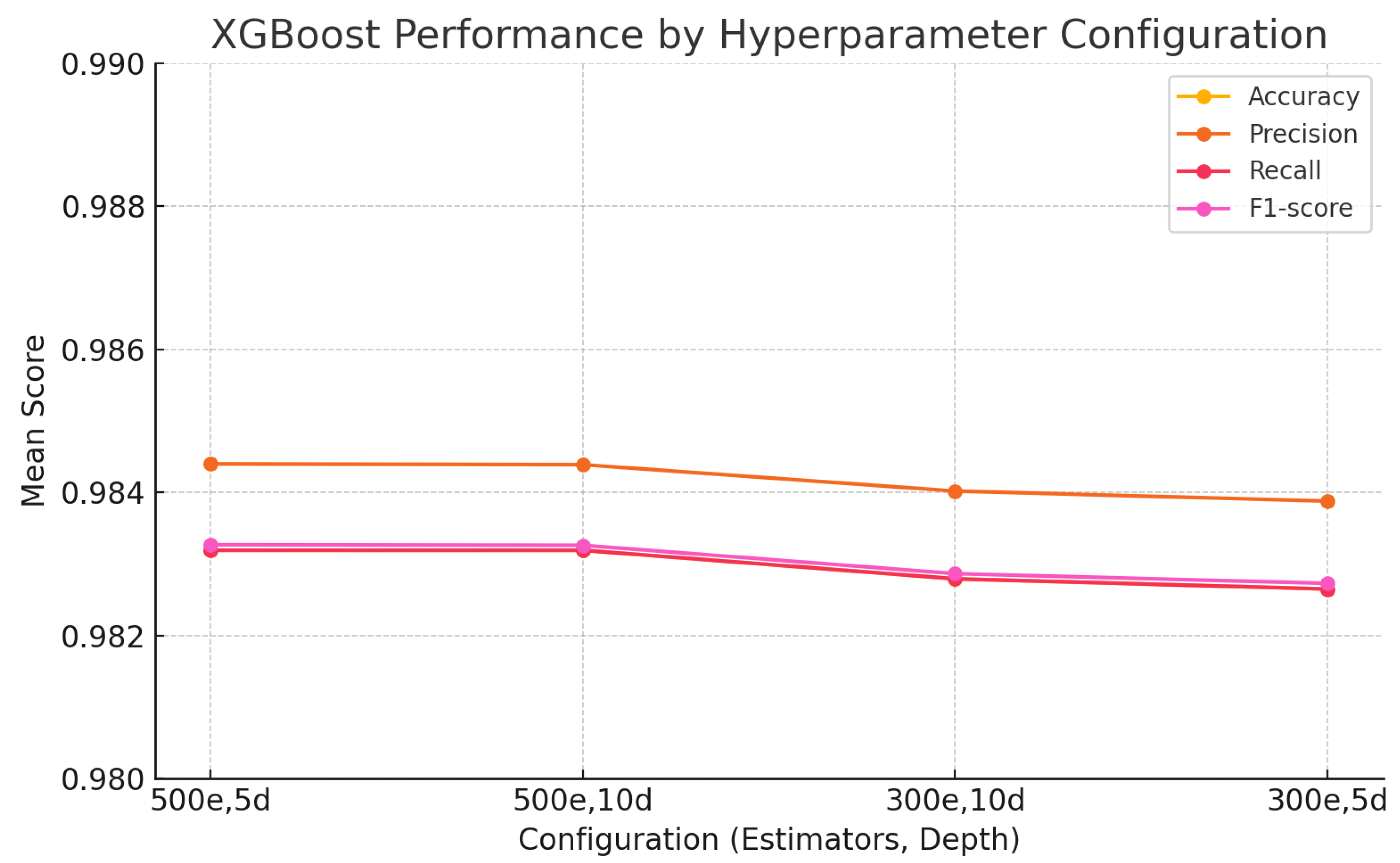
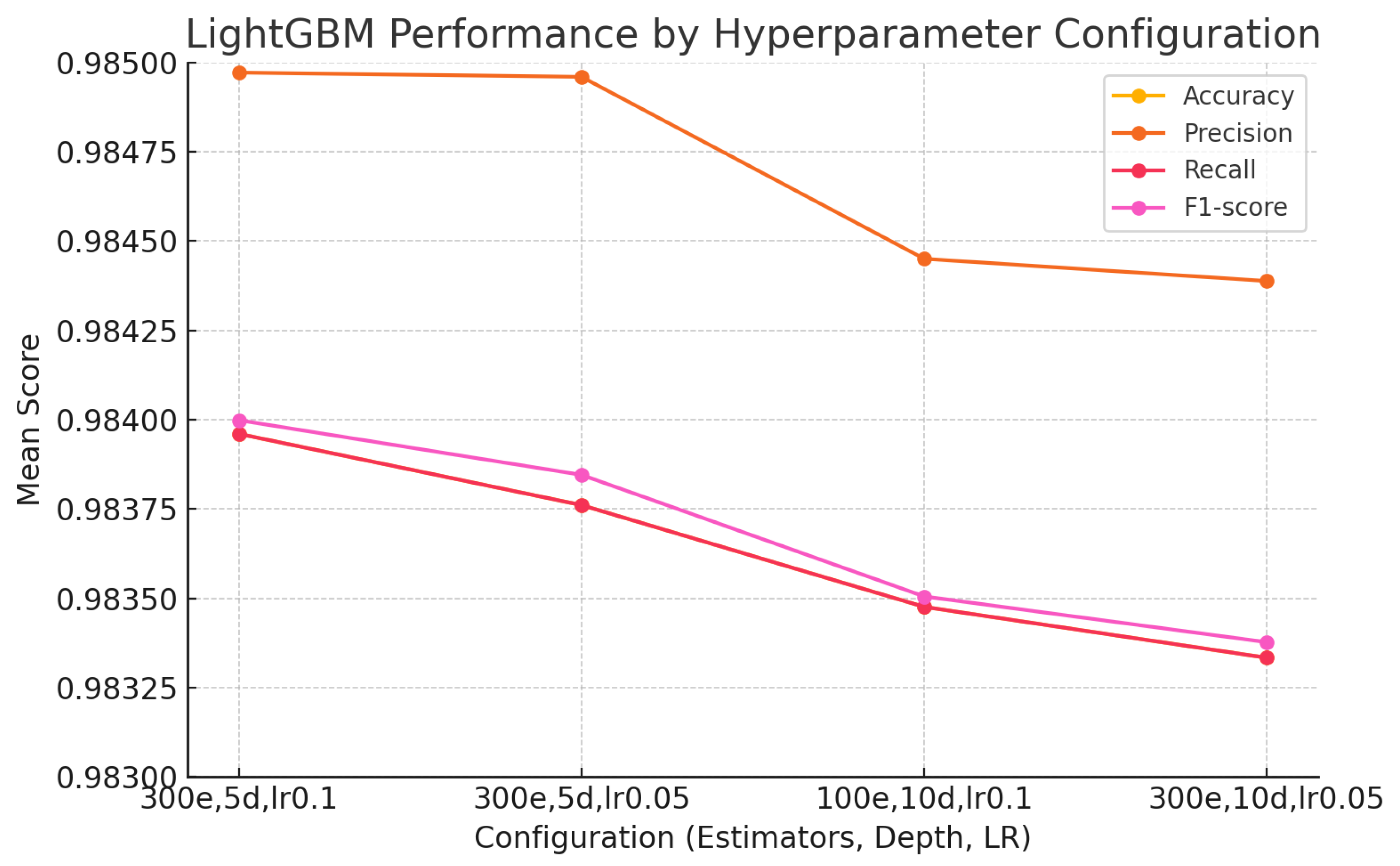
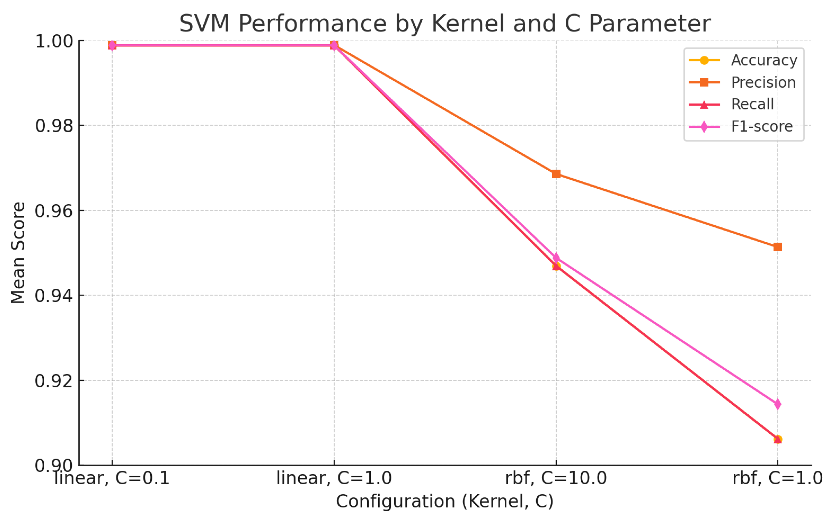
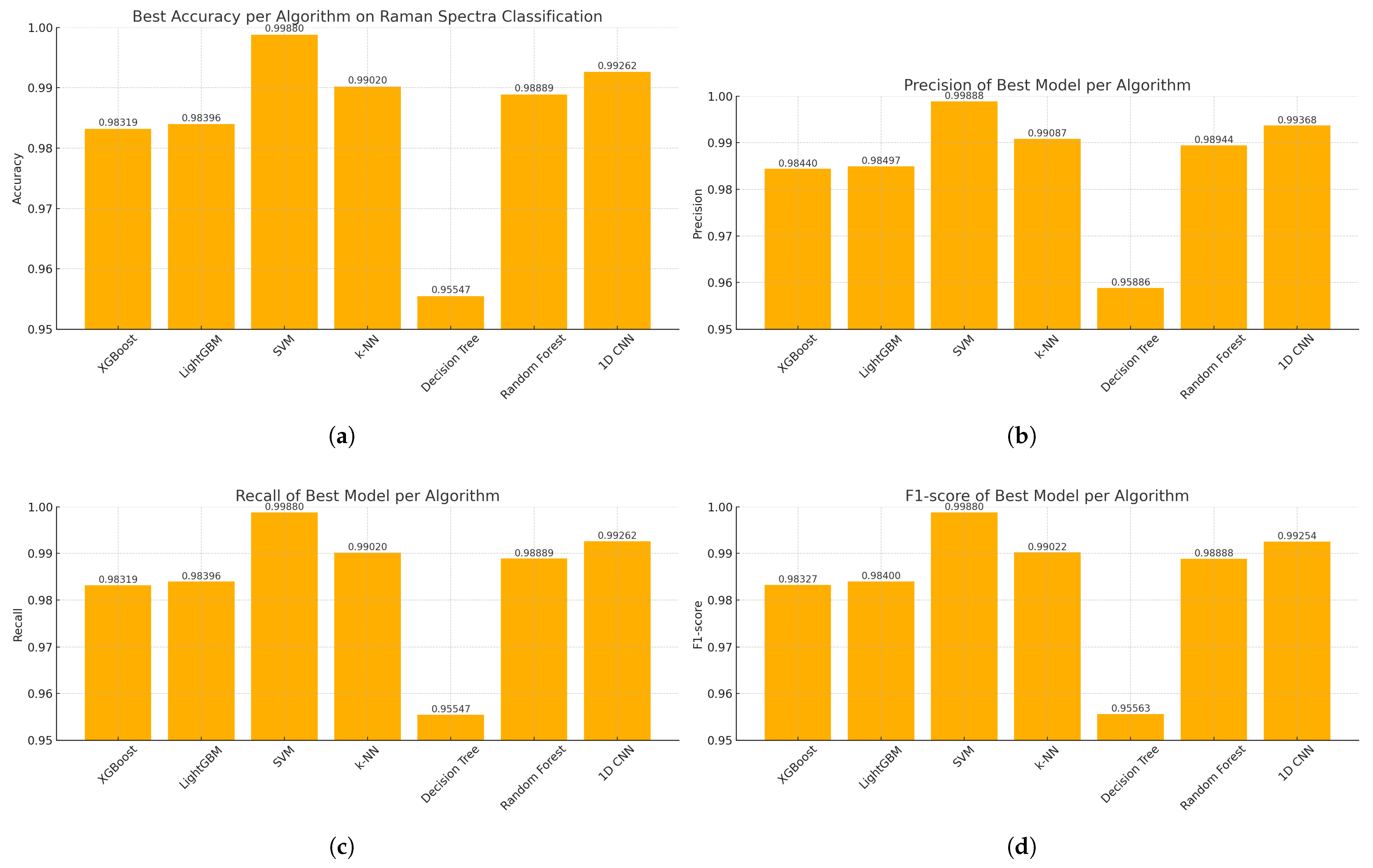
The findings of this study underscore the growing relevance of explainable machine learning techniques in the context of pharmaceutical spectroscopy. Among the evaluated models, the Support Vector Machine (SVM) with a linear kernel achieved the highest classification accuracy (99.88%), highlighting its effectiveness in handling high-dimensional spectral data when class boundaries are well defined. Meanwhile, the 1D Convolutional Neural Network (CNN) also demonstrated strong performance (accuracy of 99.26%) and offered unique advantages in terms of interpretability through SHAP-based explanations.

Notably, the SHAP heatmap generated for the CNN revealed localized spectral regions—particularly in the 300–350 cm⁻¹, 600–920 cm⁻¹ and 1050 cm⁻¹ ranges—that were consistently influential across multiple classes. These regions correspond to known Raman-active vibrational modes, indicating that the CNN model was able to autonomously learn chemically meaningful features directly from raw spectral inputs. In contrast, the SVM’s SHAP visualization exhibited a more diffuse pattern of feature importance, suggesting that while the model performed well, it distributed decision relevance more broadly across the spectrum without clear localization.

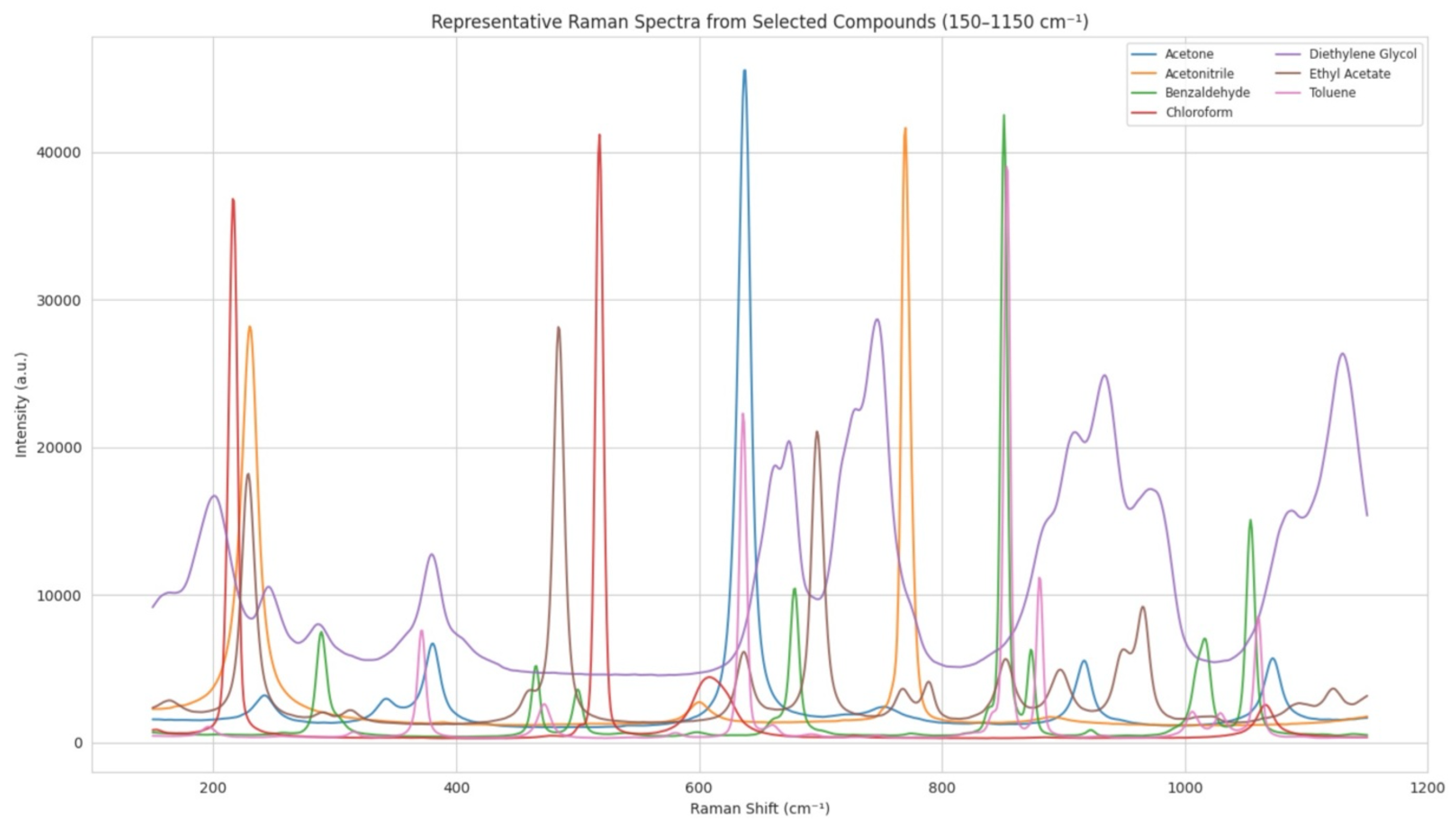
The SHAP analysis revealed that the machine learning model places significant importance on Raman shift regions that correspond to chemically meaningful vibrational modes. As detailed in

Table 10. Key Raman shift regions identified via SHAP and their corresponding chemical features.

Raman Shift (cm−1)	Associated Vibrations	Functional Structures	Example Compounds in Dataset
150–200	Ring breathing, skeletal modes	Aromatic rings, substituted benzenes	Toluene, Benzaldehyde
300–350	C–C skeletal stretch, CH2 wag	Alkanes, branched hydrocarbons	n-Hexane, n-Heptane
600–800	C–Cl, C–Br stretches; ring modes	Halogenated compounds, aromatic rings	Chloroform, Benzyl bromide
790–920	C–H out-of-plane bending	Mono- and disubstituted aromatic rings	Toluene, Benzaldehyde
1050–1150	C–O, C–N, C–C stretching	Ethers, esters, amines	Ethyl acetate, DMSO, Acetonitrile

, many of the most influential spectral regions align with characteristic functional group vibrations well documented in the Raman spectroscopy literature. For instance, the 790–920 cm⁻¹ region, which showed high SHAP values, corresponds to out-of-plane C–H bending in mono- and disubstituted aromatic rings—functional motifs frequently found in pharmacologically active compounds such as toluene derivatives. Similarly, the 1050–1150 cm⁻¹ region, associated with C–O and C–N stretching vibrations, is indicative of ether, ester, and amine functionalities, which are prevalent in a wide range of bioactive molecules and excipients. These findings not only affirm that the model is capturing structurally and pharmacologically relevant spectral features but also enhance the interpretability and mechanistic plausibility of the classification results [28,29].

This analysis revealed important spectral regions used by the model to distinguish compounds. While some of these regions correspond to well-known vibrational modes (e.g., C–O or ring deformation bands), others do not coincide with visually dominant peaks. This suggests that the model may exploit subtle, low-amplitude patterns, such as weak shoulders or overlapping bands, highlighting the potential of explainable AI to uncover latent spectral information beyond conventional inspection.

This distinction in interpretability has practical implications. In pharmaceutical quality control scenarios, where understanding which spectral regions contribute to a prediction is critical, CNN-based models may provide not only high accuracy but also actionable insights. Such transparency supports regulatory compliance, enhances trust in automated systems, and facilitates the identification of anomalies or adulterations in real-world settings.

This study demonstrates that integrating explainability tools such as SHAP with high-performing machine learning models enhances both the transparency and utility of Raman spectroscopy in pharmaceutical analysis. Future work may explore extending this framework to other spectroscopic modalities, implementing real-time classification pipelines, and expanding the chemical space to include complex formulations and biological matrices.

In future work, we plan to extend our benchmarking to include classical chemometric techniques such as Principal Component Analysis (PCA) and Linear Discriminant Analysis (LDA), which are standard tools in spectroscopy. This would allow for a direct comparison between traditional statistical approaches and machine learning models in terms of both classification performance and interpretability.

Also, we plan to extend the SHAP-based interpretation of our models by systematically analyzing whether the most influential spectral regions correspond to known vibrational modes associated with specific chemical structures. While this was not feasible in the present study due to the large number of classes (32 compounds), such analysis could be performed in focused studies with fewer, well-characterized compounds. This would enhance the interpretability of ML-based spectral classification and potentially provide new insights into structure–spectrum relationships in Raman spectroscopy.

References

1. Silge, A.; Weber, K.; Cialla-May, D.; Müller-Bötticher, L.; Fischer, D.; Popp, J. Trends in pharmaceutical analysis and quality control by modern Raman spectroscopic techniques. TrAC Trends Anal. Chem. 2022, 153, 116623. [Google Scholar] [CrossRef]
2. Inoue, M.; Hisada, H.; Koide, T.; Fukami, T.; Roy, A.; Carriere, J.; Heyler, R. Transmission Low-Frequency Raman Spectroscopy for Quantification of Crystalline Polymorphs in Pharmaceutical Tablets. Anal. Chem. 2019, 91, 1997–2003. [Google Scholar] [CrossRef] [PubMed]
3. Hess, C. New advances in using Raman spectroscopy for the characterization of catalysts and catalytic reactions. Chem. Soc. Rev. 2021, 50, 3519–3564. [Google Scholar] [CrossRef] [PubMed]
4. Han, X.X.; Rodriguez, R.S.; Haynes, C.L.; Ozaki, Y.; Zhao, B. Surface-enhanced Raman spectroscopy. Nat. Rev. Methods Prim. 2022, 1, 87. [Google Scholar] [CrossRef]
5. Sherman, A.M.; Takanti, N.; Rong, J.; Simpson, G.J. Nonlinear optical characterization of pharmaceutical formulations. TrAC Trends Anal. Chem. 2021, 140, 116241. [Google Scholar] [CrossRef]
6. Mosca, S.; Conti, C.; Stone, N.; Matousek, P. Spatially offset Raman spectroscopy. Nat. Rev. Methods Prim. 2021, 1, 21. [Google Scholar] [CrossRef]
7. Storozhuk, D.; Ryabchykov, O.; Popp, J.; Bocklitz, T. RAMANMETRIX: A delightful way to analyze Raman spectra. arXiv 2022, arXiv:2201.07586. [Google Scholar] [CrossRef]
8. Trenfield, S.J.; Januskaite, P.; Goyanes, A.; Wilsdon, D.; Rowland, M.; Gaisford, S.; Basit, A.W. Prediction of Solid-State Form of SLS 3D Printed Medicines Using NIR and Raman Spectroscopy. Pharmaceutics 2022, 14, 589. [Google Scholar] [CrossRef]
9. Cîntǎ Pînzaru, S.; Pavel, I.; Leopold, N.; Kiefer, W. Identification and characterization of pharmaceuticals using Raman and surface-enhanced Raman scattering. J. Raman Spectrosc. 2004, 35, 338–346. [Google Scholar] [CrossRef]
10. Kandpal, L.M.; Cho, B.K.; Tewari, J.; Gopinathan, N. Raman spectral imaging technique for API detection in pharmaceutical microtablets. Sens. Actuators B Chem. 2018, 260, 213–222. [Google Scholar] [CrossRef]
11. Peng, M.; Wang, Z.; Sun, X.; Guo, X.; Wang, H.; Li, R.; Liu, Q.; Chen, M.; Chen, X. Deep Learning-Based Label-Free Surface-Enhanced Raman Scattering Screening and Recognition of Small-Molecule Binding Sites in Proteins. Anal. Chem. 2022, 94, 11483–11491. [Google Scholar] [CrossRef] [PubMed]
12. Tao, Y.; Bao, J.; Liu, Q.; Liu, L.; Zhu, J. Application of Deep-Learning Algorithm Driven Intelligent Raman Spectroscopy Methodology to Quality Control in the Manufacturing Process of Guanxinning Tablets. Molecules 2022, 27, 6969. [Google Scholar] [CrossRef] [PubMed]
13. Roggo, Y.; Degardin, K.; Margot, P. Identification of pharmaceutical tablets by Raman spectroscopy and chemometrics. Talanta 2010, 81, 988–995. [Google Scholar] [CrossRef] [PubMed]
14. Galata, D.L.; Zsiros, B.; Knyihár, G.; Péterfi, O.; Mészáros, L.A.; Ronkay, F.; Nagy, B.; Szabó, E.; Nagy, Z.K.; Farkas, A. Convolutional neural network-based evaluation of chemical maps obtained by fast Raman imaging for prediction of tablet dissolution profiles. Int. J. Pharm. 2023, 640, 123001. [Google Scholar] [CrossRef] [PubMed]
15. Péterfi, O.; Nagy, Z.K.; Sipos, E.; Galata, D.L. Artificial Intelligence-based Prediction of In Vitro Dissolution Profile of Immediate Release Tablets with Near-infrared and Raman Spectroscopy. Period. Polytech. Chem. Eng. 2023, 67, 18–30. [Google Scholar] [CrossRef]
16. Sheng, H.; Zhao, Y.; Long, X.; Chen, L.; Li, B.; Fei, Y.; Mi, L.; Ma, J. Visible Particle Identification Using Raman Spectroscopy and Machine Learning. AAPS PharmSciTech 2022, 23, 186. [Google Scholar] [CrossRef]
17. Amin, M.O.; Al-Hetlani, E.; Lednev, I.K. Detection and identification of drug traces in latent fingermarks using Raman spectroscopy. Sci. Rep. 2022, 12, 3136. [Google Scholar] [CrossRef]
18. Abdalla, Y.; McCoubrey, L.E.; Ferraro, F.; Sonnleitner, L.M.; Guinet, Y.; Siepmann, F.; Hédoux, A.; Siepmann, J.; Basit, A.W.; Orlu, M.; et al. Machine learning of Raman spectra predicts drug release from polysaccharide coatings for targeted colonic delivery. J. Control. Release 2024, 374, 103–111. [Google Scholar] [CrossRef]
19. Fu, X.; Zhong, L.m.; Cao, Y.b.; Chen, H.; Lu, F. Quantitative analysis of excipient dominated drug formulations by Raman spectroscopy combined with deep learning. Anal. Methods 2021, 13, 64–68. [Google Scholar] [CrossRef]
20. Tanemura, H.; Kitamura, R.; Yamada, Y.; Hoshino, M.; Kakihara, H.; Nonaka, K. Comprehensive modeling of cell culture profile using Raman spectroscopy and machine learning. Sci. Rep. 2023, 13, 21805. [Google Scholar] [CrossRef]
21. Le, L.M.M.; Kégl, B.; Gramfort, A.; Marini, C.; Nguyen, D.; Cherti, M.; Tfaili, S.; Tfayli, A.; Baillet-Guffroy, A.; Prognon, P.; et al. Optimization of classification and regression analysis of four monoclonal antibodies from Raman spectra using collaborative machine learning approach. Talanta 2018, 184, 260–265. [Google Scholar] [CrossRef] [PubMed]
22. Flanagan, A.R.; Glavin, F.G. Open-source Raman spectra of chemical compounds for active pharmaceutical ingredient development. Sci. Data 2025, 12, 498. [Google Scholar] [CrossRef] [PubMed]
23. Rokach, L.; Maimon, O. Decision Trees. In Data Mining and Knowledge Discovery Handbook; Maimon, O., Rokach, L., Eds.; Springer: Boston, MA, USA, 2005; pp. 165–192. [Google Scholar] [CrossRef]
24. Shalev-Shwartz, S.; Ben-David, S. Understanding Machine Learning: From Theory to Algorithms; Cambridge University Press: New York, NY, USA, 2014. [Google Scholar]
25. Chen, T.; Guestrin, C. XGBoost: A Scalable Tree Boosting System. In Proceedings of the Proceedings of the 22nd ACM SIGKDD International Conference on Knowledge Discovery and Data Mining, San Francisco, CA, USA, 13–17 August 2016; KDD’16. pp. 785–794. [Google Scholar] [CrossRef]
26. Kalatzis, D.; Spyratou, E.; Karnachoriti, M.; Kouri, M.A.; Orfanoudakis, S.; Koufopoulos, N.; Pouliakis, A.; Danias, N.; Seimenis, I.; Kontos, A.G.; et al. Advanced Raman Spectroscopy Based on Transfer Learning by Using a Convolutional Neural Network for Personalized Colorectal Cancer Diagnosis. Optics 2023, 4, 310–320. [Google Scholar] [CrossRef]
27. Lundberg, S.M.; Lee, S.I. A unified approach to interpreting model predictions. In Proceedings of the Proceedings of the 31st International Conference on Neural Information Processing Systems, Long Beach, CA, USA, 4–9 December 2017; NIPS’17. pp. 4768–4777. [Google Scholar]
28. Das, R.S.; Agrawal, Y. Raman spectroscopy: Recent advancements, techniques and applications. Vib. Spectrosc. 2011, 57, 163–176. [Google Scholar] [CrossRef]
29. Smith, E.; Dent, G. Modern Raman Spectroscopy: A Practical Approach, 2nd ed.; Wiley: Chichester, UK, 2019. [Google Scholar]
Figure 1. Methodological workflow.
Eng 06 00145 g001
Figure 2. Representative Raman spectra (150–1150 cm−1) from selected compounds in the dataset, illustrating structural and spectral diversity across chemical classes (e.g., ketones, aromatics, esters, alcohols, halogenated compounds).
Eng 06 00145 g002
Figure 3. XGBoost performance by hyperparameter configuration.
Eng 06 00145 g003
Figure 4. LightGBM performance by hyperparameter configuration.
Eng 06 00145 g004
Figure 5. SVM performance by kernel and regularization parameter C.
Eng 06 00145 g005
Figure 6. k-NN performance for different ( p , k , weights ) settings.
Eng 06 00145 g006
Figure 7. Decision Tree performance for different configurations of splitting criterion, tree depth, and sample thresholds.
Eng 06 00145 g007
Figure 8. Random Forest performance for different configurations at max_depth = 10.
Eng 06 00145 g008
Figure 9. CNN performance on classification task.
Eng 06 00145 g009
Figure 10. Accuracy, precision, recall, and F1-score for the best configuration of each algorithm: (a) The accuracy for the best configuration of each algorithm. (b) The precision for the best configuration of each algorithm. (c) The recall for the best configuration of each algorithm. (d) The F1-score for the best configuration of each algorithm.
Eng 06 00145 g010
Figure 11. SHAP heatmaps comparing feature attributions across 32 classes for SVM and CNN models applied to Raman spectra. (a) SHAP heatmap of CNN (b) SHAP heatmap of SVM.
Eng 06 00145 g011