
Low-Observability Distribution System State Estimation by Graph Computing with Enhanced Numerical Stability

Abstract
1. Introduction
2. Basic Principles of SE
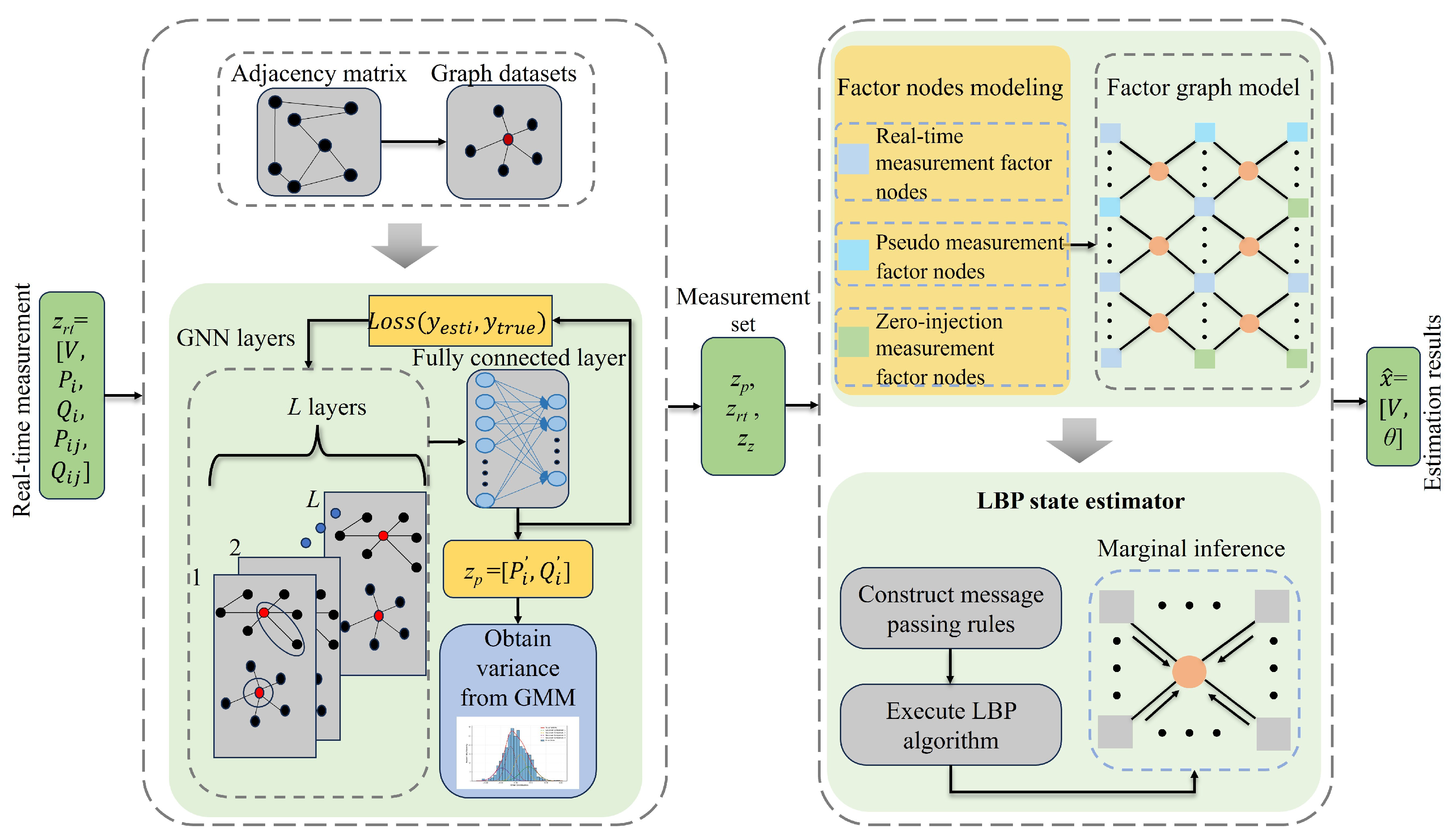
3. Fully Distributed SE with GNN-Based Pseudo-Measurements
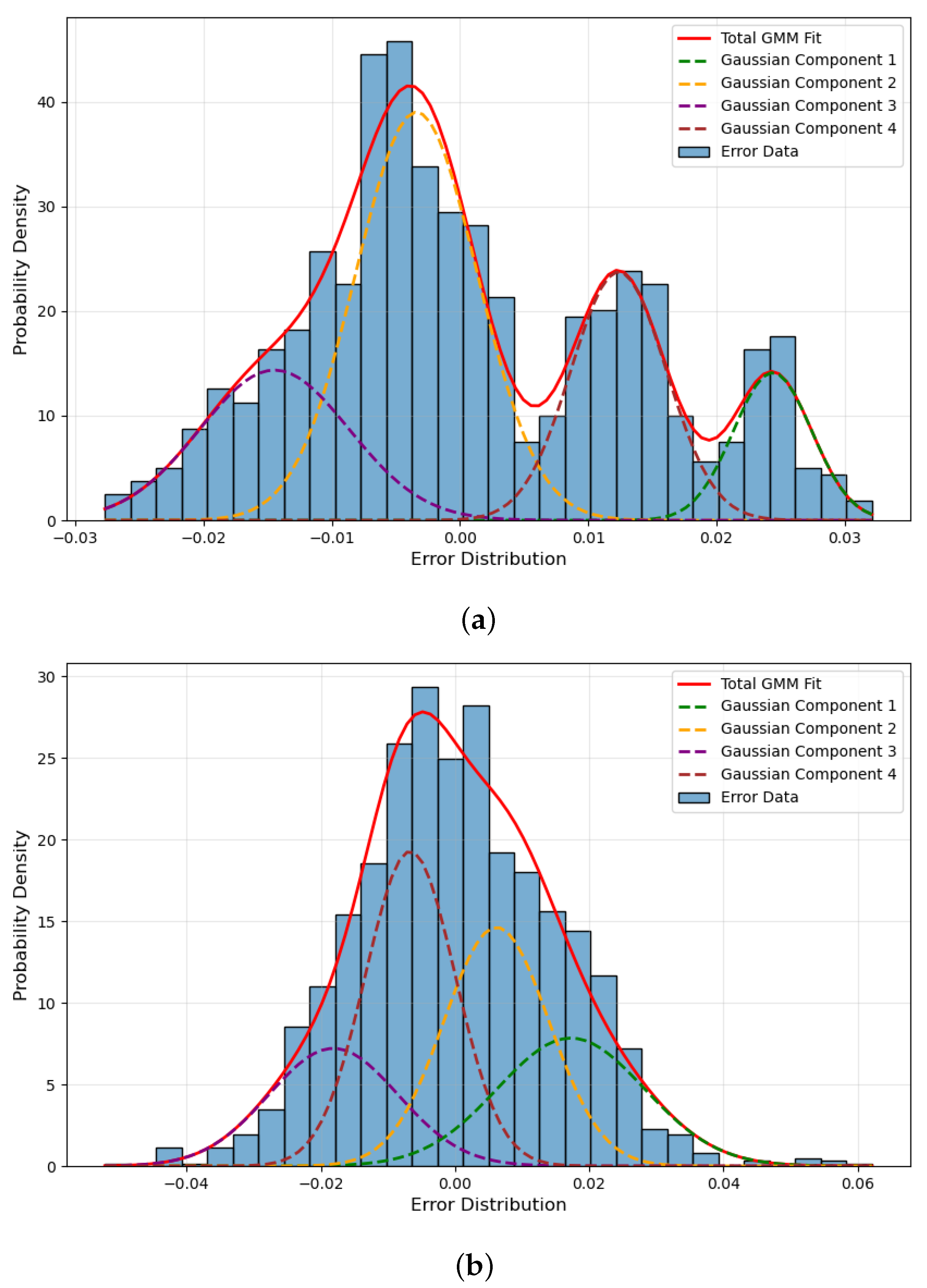
3.1. GNN-Based Pseudo-Measurement Modeling
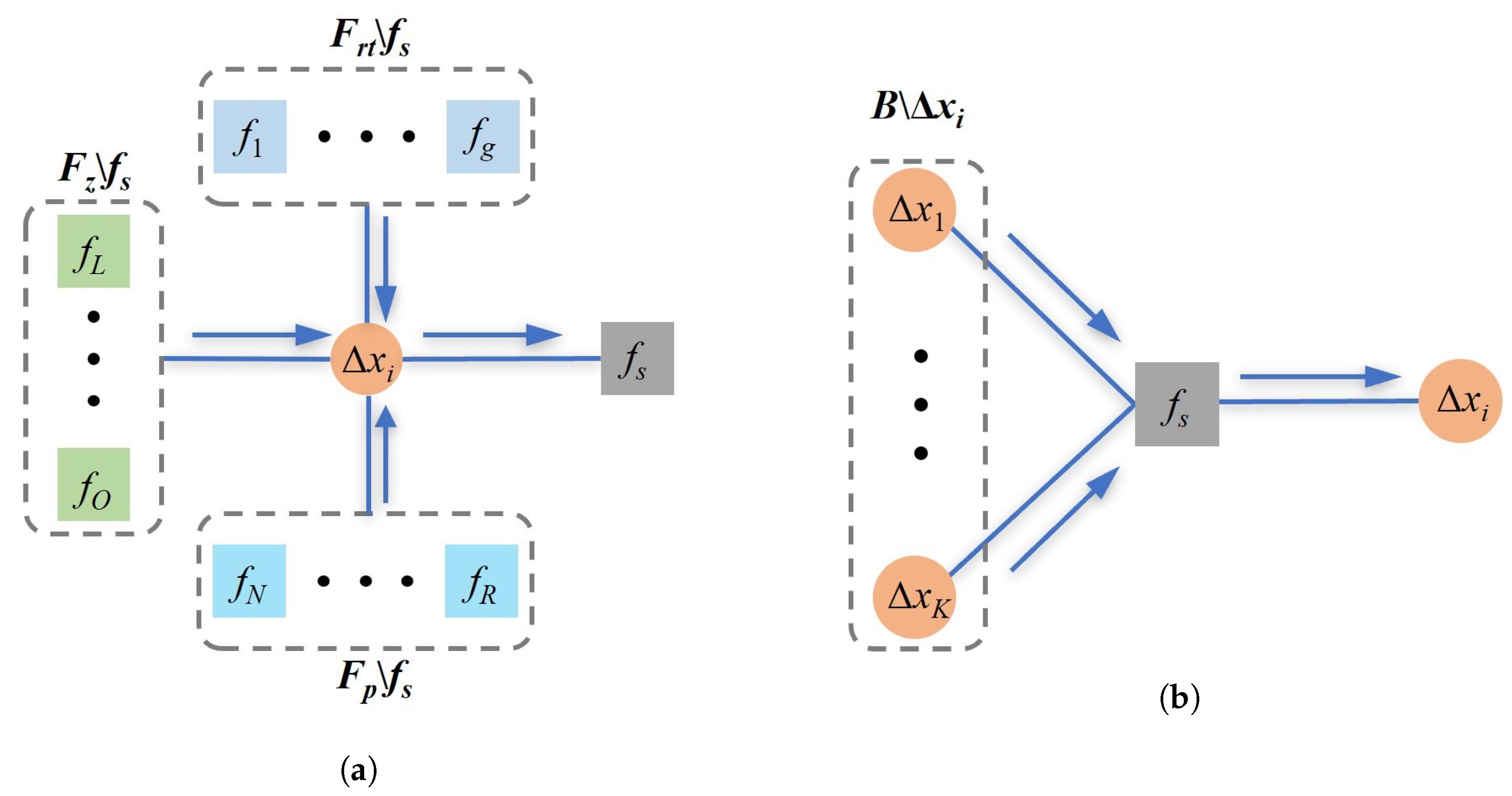
3.2. Factor Graph-Based Fully Distributed SE for Distribution Systems
4. Case Study
4.1. Accuracy Evaluation of Pseudo-Measurement Modeling
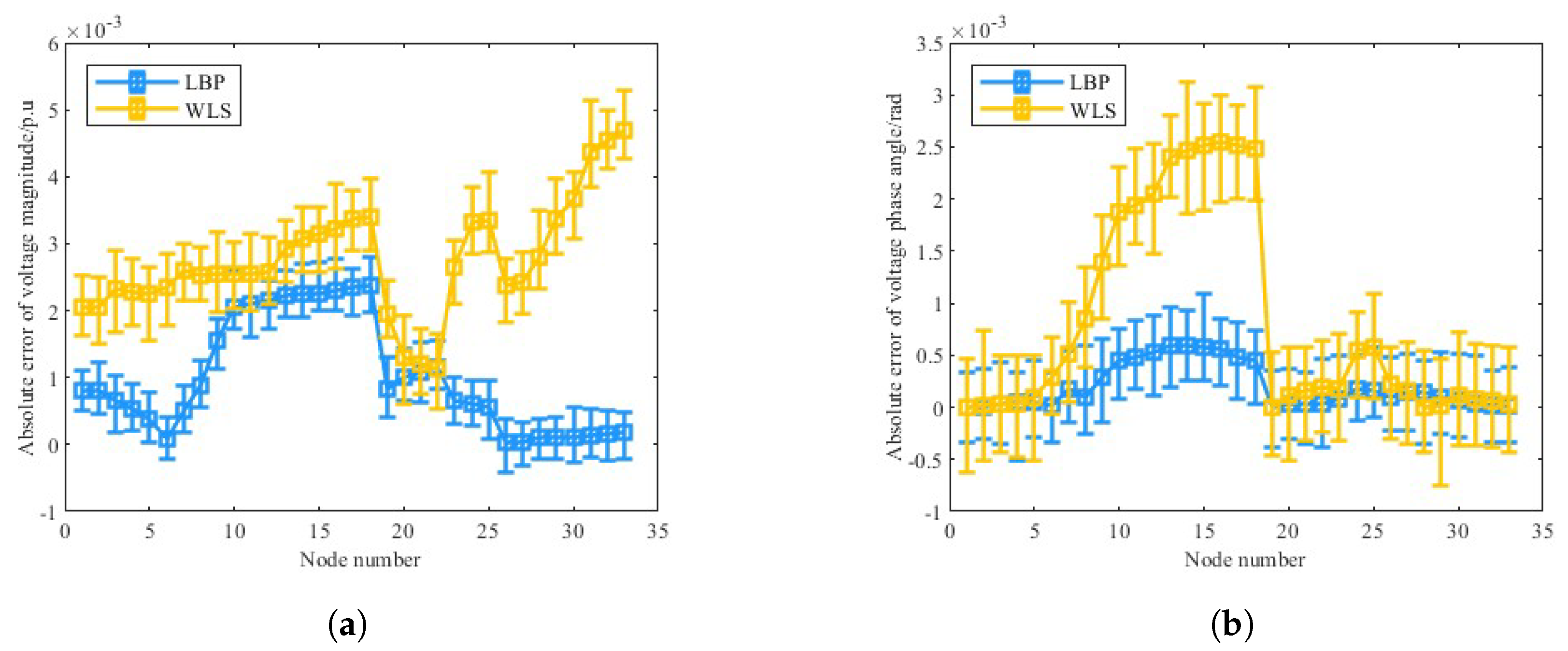
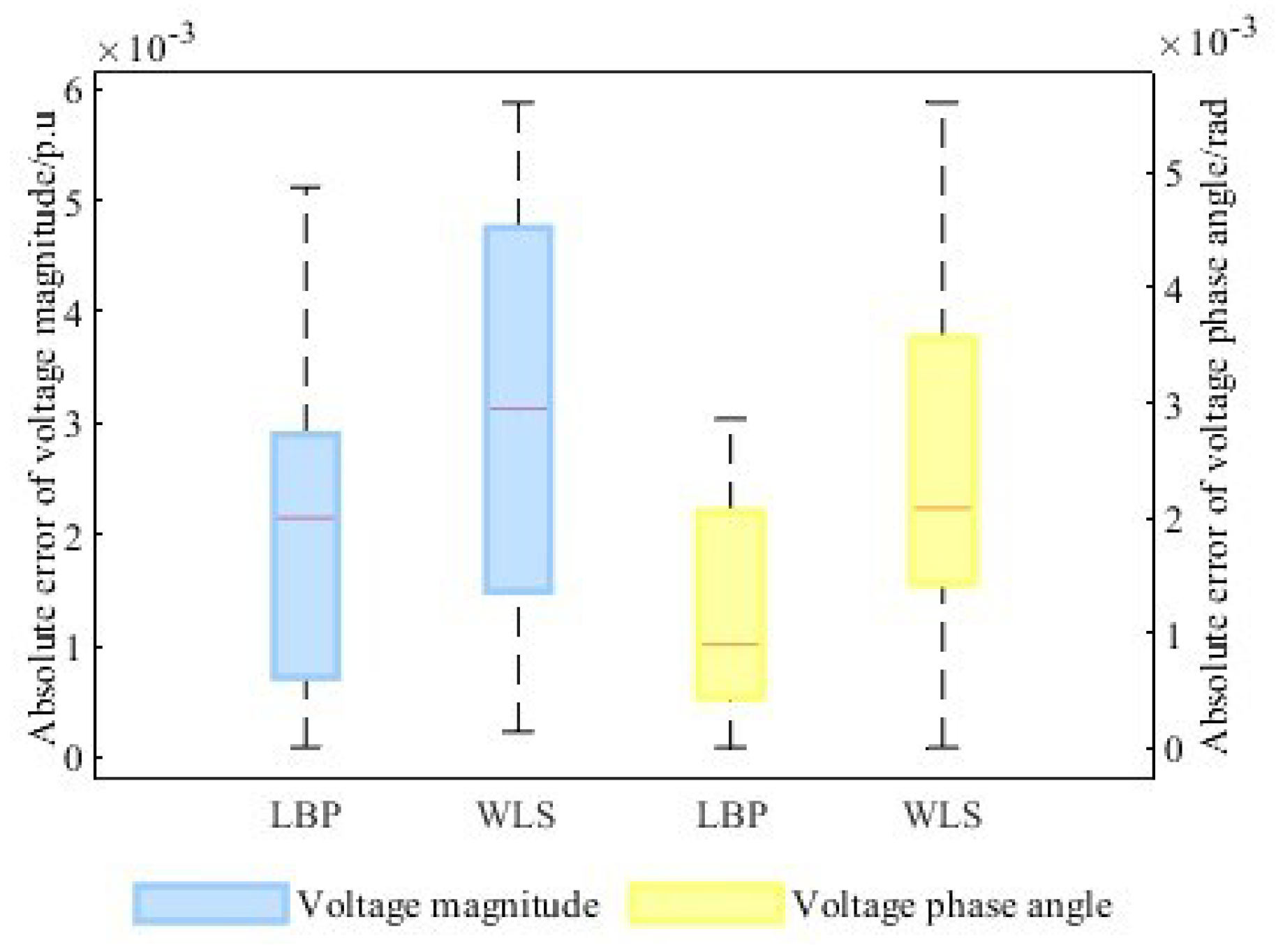
4.2. Accuracy Evaluation of LBP with Pseudo-Measurements
- 1.
- Normal noise scenario: the standard deviation of voltage magnitude, injection power, and branch power are set to 0.5%, 1%, and 1%, respectively.
- 2.
- High noise scenario: the standard deviation of voltage magnitude is increased to 1%, while the standard deviations of injection power and branch power are both increased to 10%.
5. Conclusions
Author Contributions
Funding
Institutional Review Board Statement
Informed Consent Statement
Data Availability Statement
Conflicts of Interest
Appendix A
References
- Bardhi, A.; Eski, A.; Leka, B.; Dhoska, K. The Impact of Solar Power Plants on the Electricity Grid: A Case Study of Albania. Eng 2025, 6, 35. [Google Scholar] [CrossRef]
- Soto, E.A.; Bosman, L.B.; Wollega, E.; Leon-Salas, W.D. Analysis of Grid Disturbances Caused by Massive Integration of Utility Level Solar Power Systems. Eng 2022, 3, 236–253. [Google Scholar] [CrossRef]
- Ramachandran, T.; Reiman, A.; Nandanoori, S.P.; Rice, M.; Kundu, S. Distribution System State Estimation in the Presence of High Solar Penetration. In Proceedings of the 2019 American Control Conference (ACC), Philadelphia, PA, USA, 10–12 July 2019; pp. 3432–3437. [Google Scholar]
- Medvedieva, K.; Tosi, T.; Barbierato, E.; Gatti, A. Balancing the Scale: Data Augmentation Techniques for Improved Supervised Learning in Cyberattack Detection. Eng 2024, 5, 2170–2205. [Google Scholar] [CrossRef]
- Primadianto, A.; Lu, C.-N. A Review on Distribution System State Estimation. IEEE Trans. Power Syst. 2017, 32, 3875–3883. [Google Scholar] [CrossRef]
- Dehghanpour, K.; Wang, Z.; Wang, J.; Yuan, Y.; Bu, F. A Survey on State Estimation Techniques and Challenges in Smart Distribution Systems. IEEE Trans. Smart Grid 2019, 10, 2312–2322. [Google Scholar] [CrossRef]
- Yu, Y.; Jin, Z.; Ćetenović, D.; Ding, L.; Levi, V.; Terzija, V. A Robust Distribution Network State Estimation Method Based on Enhanced Clustering Algorithm: Accounting for Multiple DG Output Modes and Data Loss. Int. J. Electr. Power Energy Syst. 2024, 157, 109797. [Google Scholar] [CrossRef]
- Ju, Y.; Jia, X.; Wang, B. Review of Dataset and Algorithms for Distribution Network Pseudo Measurement. Energy Internet 2024, 2, 1–12. [Google Scholar] [CrossRef]
- Manitsas, E.; Singh, R.; Pal, B.; Strbac, G. Modelling of Pseudo-Measurements for Distribution System State Estimation. In Proceedings of the CIRED Seminar 2008: SmartGrids for Distribution, Frankfurt, Germany, 23–24 June 2008. [Google Scholar]
- Wang, S.; Zhao, J.; Huang, Z.; Diao, R. Assessing Gaussian Assumption of PMU Measurement Error Using Field Data. IEEE Trans. Power Del. 2018, 33, 3233–3236. [Google Scholar] [CrossRef]
- Xu, D.L.; Wu, Z.J.; Xu, J.J.; Hu, Q.R. A Pseudo Measurement Modeling Based Forecasting Aided State Estimation Framework for Distribution Network. Int. J. Electr. Power Energy Syst. 2024, 160, 110116. [Google Scholar] [CrossRef]
- Xu, D.; Xu, J.; Qian, C.; Wu, Z.; Hu, Q. A Pseudo-Measurement Modelling Strategy for Active Distribution Networks Considering Uncertainty of DGs. Prot. Control Mod. Power Syst. 2024, 9, 1–15. [Google Scholar] [CrossRef]
- Manitsas, E.; Singh, R.; Pal, B.C.; Strbac, G. Distribution System State Estimation Using an Artificial Neural Network Approach for Pseudo Measurement Modeling. IEEE Trans. Power Syst. 2012, 27, 1888–1896. [Google Scholar] [CrossRef]
- Wang, Y.; Gu, J.; Yuan, L. Distribution Network State Estimation Based on Attention-Enhanced Recurrent Neural Network Pseudo-Measurement Modeling. Prot. Control Mod. Power Syst. 2023, 8, 31. [Google Scholar] [CrossRef]
- Qiang, Q.; Guoqiang, S.; Wei, X.; Minghui, Y.; Zhinong, W.; Haixiang, Z. Distribution System State Estimation Based on Pseudo Measurement Modeling Using Convolutional Neural Network. In Proceedings of the 2018 China International Conference on Electricity Distribution (CICED), Tianjin, China, 17–19 September 2018; pp. 2416–2420. [Google Scholar]
- Cooper, A.; Bretas, A.; Meyn, S. Anomaly Detection in Power System State Estimation: Review and New Directions. Energies 2023, 16, 6678. [Google Scholar] [CrossRef]
- Wu, L.; Wang, Y.; Wang, Y.; Si, J. Cellular Computational Networks Based Hierarchical Data-Driven Dynamic State Estimation Method Considering Uncertainties. Prot. Control Mod. Power Syst. 2025, 10, 150–161. [Google Scholar] [CrossRef]
- Chen, B.; Li, H.; Su, X. Dynamic State Estimation of Distribution Network Base on Pseudo Measurement Modeling and UPF. In Proceedings of the 2019 IEEE Innovative Smart Grid Technologies—Asia (ISGT Asia), Chengdu, China, 21–24 May 2019; pp. 54–59. [Google Scholar]
- Wang, Y.; Xia, M.; Chen, Q.; Chen, F.; Yang, X.; Han, F. Fast State Estimation of Power System Based on Extreme Learning Machine Pseudo-Measurement Modeling. In Proceedings of the 2019 IEEE Innovative Smart Grid Technologies—Asia (ISGT Asia), Chengdu, China, 21–24 May 2019; pp. 1236–1241. [Google Scholar]
- Chen, D.; Xu, J.; Wu, X.; Che, Y. Distribution Network State Estimation Based on CNN-LSTM Pseudo-Measurement Model. In Proceedings of the 2023 International Conference on Power System Technology (PowerCon), Jinan, China, 21–22 September 2023; pp. 1–5. [Google Scholar]
- Schweppe, F.; Wildes, J. Power System Static-State Estimation, Part I: Exact Model. IEEE Trans. Power App. Syst. 1970, PAS-89, 120–125. [Google Scholar] [CrossRef]
- Poursaeed, A.H.; Namdari, F. Online Transient Stability Assessment Implementing the Weighted Least-Square Support Vector Machine with the Consideration of Protection Relays. Prot. Control Mod. Power Syst. 2025, 10, 1–17. [Google Scholar] [CrossRef]
- Khare, G.; Mohapatra, A.; Singh, S.N. State vulnerability assessment against false data injection attacks in AC state estimators. Energy Convers. Econ. 2022, 3, 319–332. [Google Scholar] [CrossRef]
- Wang, L.; Zhou, Q.; Jin, S. Physics-guided Deep Learning for Power System State Estimation. J. Mod. Power Syst. Clean Energy 2020, 8, 607–615. [Google Scholar] [CrossRef]
- Liu, Z.; Li, P.; Wang, C.; Yu, H.; Ji, H.; Xi, W.; Wu, J. Robust State Estimation of Active Distribution Networks with Multi-source Measurements. J. Mod. Power Syst. Clean Energy 2023, 11, 1540–1552. [Google Scholar] [CrossRef]
- Yu, Y.; Wang, Y. Enabling Forecasting-Aided State Estimation in Active Distribution Networks via GRformer-Driven Pseudo-Measurement Modeling. In Proceedings of the 2024 IEEE/IAS Industrial and Commercial Power System Asia (I&CPS Asia), Pattaya, Thailand, 9–12 July 2024; pp. 80–84. [Google Scholar]
- Wu, Z.; Pan, S.; Chen, F.; Long, G.; Zhang, C.; Yu, P.S. A Comprehensive Survey on Graph Neural Networks. IEEE Trans. Neural Netw. Learn. Syst. 2021, 32, 4–24. [Google Scholar] [CrossRef]
- Bronstein, M.M.; Bruna, J.; Cohen, T.; Veličković, P. Geometric Deep Learning: Grids, Groups, Graphs, Geodesics, and Gauges. arXiv 2021, arXiv:2104.13478. [Google Scholar]
- Park, H.; Sohn, K.; Lee, Y.; Kim, J.; Back, J. Distributed State Estimation for Power Systems Based on Graph Convolutional Networks. IEEE Access 2021, 9, 127689–127699. [Google Scholar]
- Lin, Y.; Sun, H.; Wang, B.; Zhang, W. EleGNN: Physics-Informed Graph Neural Network for Distribution System State Estimation. IEEE Trans. Power Syst. 2023, 38, 1440–1450. [Google Scholar]
- Hu, Y.; Kuh, A.; Yang, T.; Kavcic, A. A Belief Propagation Based Power Distribution System State Estimator. IEEE Comput. Intell. Mag. 2011, 6, 36–46. [Google Scholar] [CrossRef]
- Cosovic, M.; Vukobratovic, D. State Estimation in Electric Power Systems Using Belief Propagation: An Extended DC Model. In Proceedings of the 2016 IEEE 17th International Workshop on Signal Processing Advances in Wireless Communications (SPAWC), Edinburgh, UK, 3–6 July 2016; pp. 1–5. [Google Scholar]
- Cosovic, M.; Vukobratovic, D. Fast Real-Time DC State Estimation in Electric Power Systems Using Belief Propagation. In Proceedings of the 2017 IEEE International Conference on Smart Grid Communications (SmartGridComm), Dresden, Germany, 23–27 October 2017; pp. 207–212. [Google Scholar]
- Cosovic, M.; Vukobratovic, D. Large-Scale Multi-Area State Estimation from Phasor Measurement Units Utilizing Factor Graphs. In Proceedings of the 2019 IEEE EUROCON—18th International Conference on Smart Technologies, Novi Sad, Serbia, 1–4 July 2019; pp. 1–8. [Google Scholar]
- Zivojevic, D.; Delalic, M.; Raca, D.; Vukobratovic, D.; Cosovic, M. Distributed Weighted Least-Squares and Gaussian Belief Propagation: An Integrated Approach. In Proceedings of the 2021 IEEE International Conference on Communications, Control, and Computing Technologies for Smart Grids (SmartGridComm), Aachen, Germany, 25–28 October 2021; pp. 432–437. [Google Scholar]
- Ihler, A.T.; Fisher III, J.W.; Willsky, A.S. Loopy Belief Propagation: Convergence and Effects of Message Errors. J. Mach. Learn. Res. 2005, 6, 905–936. [Google Scholar]
- Tatikonda, S.; Jordan, M.I. Loopy Belief Propagation and Gibbs Measures. In Proceedings of the 18th Conference on Uncertainty in Artificial Intelligence (UAI), Edmonton, Canada, 1–4 August 2002; pp. 493–500. [Google Scholar]
- Cosovic, M.; Vukobratovic, D.; Stankovic, V. Linear State Estimation via 5G C-RAN Cellular Networks Using Gaussian Belief Propagation. In Proceedings of the 2018 IEEE Wireless Communications and Networking Conference (WCNC), Barcelona, Spain, 15–18 April 2018; pp. 1–6. [Google Scholar]
- Sun, K.; Wei, Z.; Dinavahi, V.; Huang, M.; Sun, G. A Complex Domain Gaussian Belief Propagation Method for Fully Distributed State Estimation. IEEE Trans. Power Syst. 2025, 40, 982–995. [Google Scholar] [CrossRef]
- Chen, Y.; Gao, Y.; Gan, K.; Li, M.; Wei, C.; Guo, X.; Zhao, R.; Lu, J.; Che, L. State Estimation for Active Distribution Networks Considering Bad Data in Measurements and Topology Parameters. Energies 2025, 18, 2222. [Google Scholar] [CrossRef]
- Jin, T.; Shen, X. A Mixed WLS Power System State Estimation Method Integrating a Wide-Area Measurement System and SCADA Technology. Energies 2018, 11, 408. [Google Scholar] [CrossRef]
- Gilmer, J.; Schoenholz, S.S.; Riley, P.F.; Vinyals, O.; Dahl, G.E. Neural Message Passing for Quantum Chemistry. In Proceedings of the 34th International Conference on Machine Learning, Sydney, Australia, 6–11 August 2017; Volume 70, pp. 1263–1272. [Google Scholar]
- Singh, R.; Pal, B.C.; Jabr, R.A. Distribution System State Estimation through Gaussian Mixture Model of the Load as Pseudo-Measurement. IET Gener. Transm. Distrib. 2010, 4, 50–59. [Google Scholar] [CrossRef]
- Pernkopf, F.; Bouchaffra, D. Genetic-Based EM Algorithm for Learning Gaussian Mixture Models. IEEE Trans. Pattern Anal. Mach. Intell. 2005, 27, 1344–1348. [Google Scholar] [CrossRef]
- Cosovic, M.; Vukobratovic, D. Distributed Gauss—Newton Method for State Estimation Using Belief Propagation. IEEE Trans. Power Syst. 2019, 34, 648–658. [Google Scholar] [CrossRef]


| Test System | Case Index | Closed Switches | Open Switches |
|---|---|---|---|
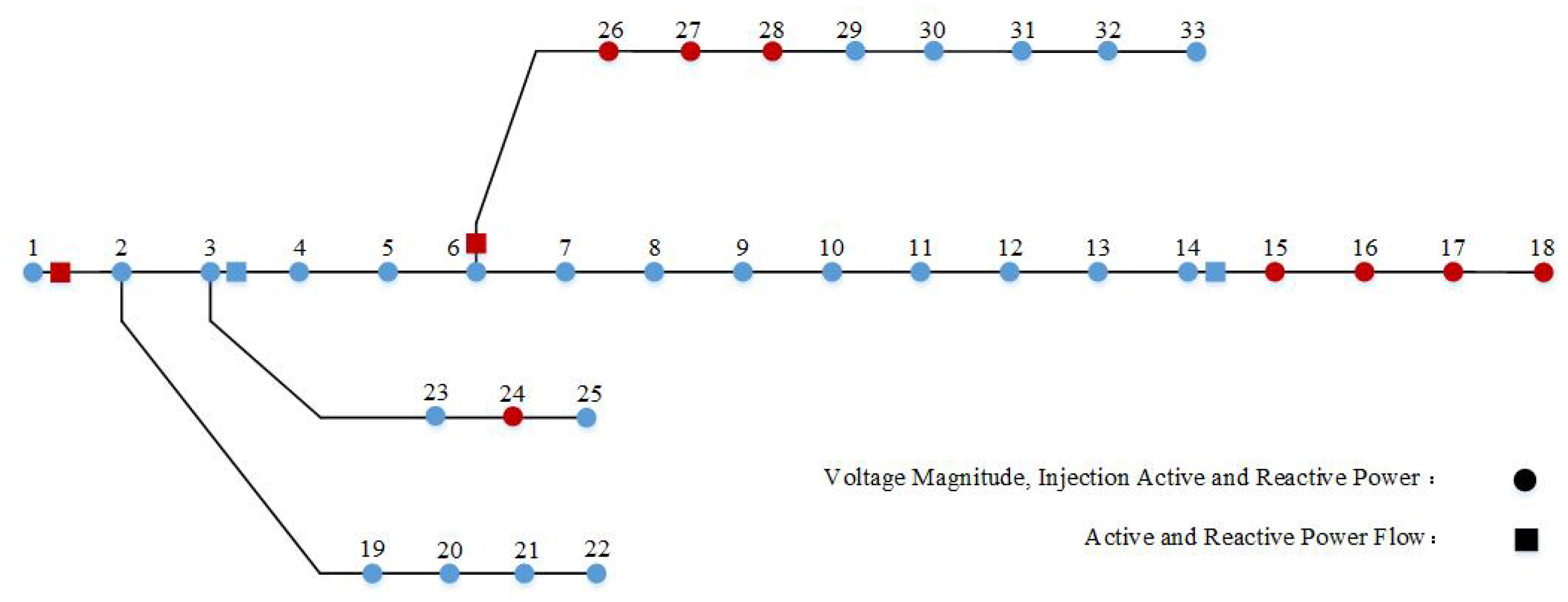
| IEEE 33-bus | 1 | 21–8, 9–15, 25–29 | 12–22, 18–33 |
| 2 | 21–8, 9–15 | 12–22, 18–33, 25–29 | |
| 3 | 12–22, 18–33, 25–29 | 9–15, 21–8 | |
| 4 | All switches | — | |
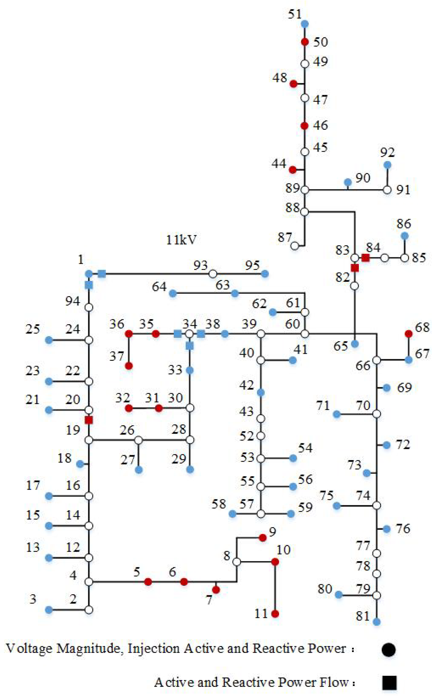
| IEEE 95-bus | 1 | 39–60, 41–65, 65–82 | 19–26 |
| 2 | 39–60, 30–33 | 65–82 | |
| 3 | 19–26, 30–33 | 39–60 | |
| 4 | 65–82, 19–26, 30–33 | 41–65 |
| System | Measurement Type | Measurement Location (Bus/Branch) | Standard Deviation |
|---|---|---|---|
| IEEE 33-bus | Voltage magnitude and bus injection power | 1–33 | Voltage magnitude: 0.5%, Power: 1% |
| Missing data | 15, 16, 17, 18, 24, 26, 27, 28 (8) | — | |
| Power flow | 1–2, 3–4, 14–15, 6–26 | 1% | |
| Missing data | 3–14, 14–15 (2) | — | |
| IEEE 95-bus | Voltage magnitude and bus injection power | 1, 3, 5, 6, 7, 9, 10, 11, 13, 15, 17, 18, 21, 23, 25, 27, 29, 31, 32, 33, 35, 36, 37, 38, 41, 42, 44, 46, 48, 50, 51, 54, 56, 58, 59, 62, 63, 64, 65, 67, 68, 69, 71, 72, 73, 75, 76, 80, 81, 86, 90, 92, 95 (53) | Voltage magnitude: 0.5%, Power: 1% |
| Missing data | 15, 16, 17, 18, 24, 26, 27, 28 (8) | — | |
| Power flow | 1–93, 1–94, 20–19, 34–35, 34–33, 34–38, 83–82, 83–83, 83–84 (8) | 1% | |
| Missing data | 20–19, 83–82, 83–82, 83–84 (3) | — |
| Systems | IEEE 33-Bus | IEEE 95-Bus | ||
|---|---|---|---|---|
| Proposed | DNN | Proposed | DNN | |
| P Pseudo | 12.451% | 17.213% | 14.074% | 18.249% |
| Q Pseudo | 15.238% | 18.135% | 16.752% | 20.365% |
| Algorithm | IEEE 33-Bus | IEEE 95-Bus | ||
|---|---|---|---|---|
| LBP | ||||
| WLS | ||||
| Algorithm | IEEE 33-Bus | IEEE 95-Bus | ||
|---|---|---|---|---|
| LBP | ||||
| WLS | ||||
Disclaimer/Publisher’s Note: The statements, opinions and data contained in all publications are solely those of the individual author(s) and contributor(s) and not of MDPI and/or the editor(s). MDPI and/or the editor(s) disclaim responsibility for any injury to people or property resulting from any ideas, methods, instructions or products referred to in the content. |
© 2025 by the authors. Licensee MDPI, Basel, Switzerland. This article is an open access article distributed under the terms and conditions of the Creative Commons Attribution (CC BY) license (https://creativecommons.org/licenses/by/4.0/).
Share and Cite
Hu, Z.; Zhu, H.; Lan, L.; Xu, H.; Liu, Z.; Li, K.; Li, J.; Wei, Z. Low-Observability Distribution System State Estimation by Graph Computing with Enhanced Numerical Stability. Eng 2025, 6, 134. https://doi.org/10.3390/eng6070134
Hu Z, Zhu H, Lan L, Xu H, Liu Z, Li K, Li J, Wei Z. Low-Observability Distribution System State Estimation by Graph Computing with Enhanced Numerical Stability. Eng. 2025; 6(7):134. https://doi.org/10.3390/eng6070134
Chicago/Turabian StyleHu, Zijian, Hong Zhu, Lan Lan, Honghua Xu, Zichen Liu, Kexin Li, Jie Li, and Zhinong Wei. 2025. "Low-Observability Distribution System State Estimation by Graph Computing with Enhanced Numerical Stability" Eng 6, no. 7: 134. https://doi.org/10.3390/eng6070134
APA StyleHu, Z., Zhu, H., Lan, L., Xu, H., Liu, Z., Li, K., Li, J., & Wei, Z. (2025). Low-Observability Distribution System State Estimation by Graph Computing with Enhanced Numerical Stability. Eng, 6(7), 134. https://doi.org/10.3390/eng6070134