Article

Dynamics of a Wind-Driven Lotka–Volterra Amensalism System with Non-Selective Harvesting: Theoretical Analysis and Ecological Implications

by
Qin Yue
1,†,
Taimiao Bi
2,† and
Fengde Chen
3,*,†
1
School of Finance and Mathematics, West Anhui University, Lu’an 237012, China
2
Anhui Provincial Key Laboratory of Philosophy and Social Sciences for Data Intelligence and Rural Revitalization of Dabie Mountains, West Anhui University, Lu’an 237012, China
3
School of Mathematics and Statistics, Fuzhou University, Fuzhou 350016, China
*
Author to whom correspondence should be addressed.
These authors contributed equally to this work.
Eng 2025, 6(12), 367; https://doi.org/10.3390/eng6120367
Submission received: 17 November 2025 / Revised: 8 December 2025 / Accepted: 12 December 2025 / Published: 15 December 2025
(This article belongs to the Section Chemical, Civil and Environmental Engineering)

Abstract

This study investigates the dynamic behavior of a Lotka–Volterra amensalism system subject to non-selective harvesting, regulated by wind speed. We develop a coupled windharvesting population model that captures the dual regulatory mechanism of wind as an environmental factor on the marine ecosystem: it weakens the amensalistic interaction between species by enhancing the dilution of inhibitory substances while simultaneously suppressing human harvesting intensity by impeding fishing operations. Using stability theory and the Lyapunov function method, we systematically analyze the existence and stability of equilibrium points and explore the ecological state transitions driven by varying wind speed. The results show that the system admits four possible equilibrium states. Among them, the positive equilibrium, whenever it exists, is globally asymptotically stable. As wind speed increases, the system undergoes sequential ecological regime shifts: from extinction of both species to dominance by a single species and finally to stable coexistence of both species. Numerical simulations confirm the theoretical findings and reveal the intrinsic mechanism by which wind promotes biodiversity: by reducing harvesting pressure and mitigating the amensalistic effect. The concept of critical wind speed proposed in this work offers a quantitative basis for managing wind conditions in marine protected areas and designing adaptive harvesting strategies, holding significant implications for marine conservation and sustainable fishery development.

1. Introduction

Amensalism, as a fundamental mode of interspecific interaction, describes an ecological relationship where one species inhibits another while remaining unaffected itself. This asymmetric mechanism is widely observed in marine ecosystems, microbial communities, insect communities, and plant populations [1,2,3,4,5,6,7,8]. In recent years, many scholars have proposed various amensalism population models from the perspective of mathematical modeling and explored their diverse dynamic behaviors [9,10,11,12,13,14,15,16,17,18,19,20,21,22,23,24,25,26,27,28,29,30,31,32,33,34,35,36,37,38,39,40,41,42,43,44,45,46,47,48,49,50,51,52,53,54,55,56,57,58]. Among these studies, the foundational Lotka–Volterra amensalism model has been extended along several key dimensions to incorporate greater ecological realism.
First, substantial efforts have focused on integrating various biological mechanisms. These include the Allee effect [18,21,22,24,26,27,44], which can alter extinction thresholds; fear effects [12,40,44,45], which introduce non-consumptive physiological costs; and stage structure [28] with nonlinear birth rates [22,55], which captures ontogenetic shifts in population dynamics.
Second, the formulation of species interactions has been refined through the incorporation of different functional responses [11,14,18,21,33,34,35,36,37,39,46] and refuge effects [13,29,30,33,38,42,44,56], which modulate the intensity of amensalism under varying environmental contexts.
Third, temporal dynamics have been enriched by considering time delays [19,20,31,32] that can induce oscillatory behaviors, impulsive effects [54] representing periodic disturbances, and discrete-time systems [14,48] that better align with certain sampling regimes.
Finally, the crucial impact of human activities has been examined through various harvesting strategies [10,25,26,29,47,49,52,53], while more complex community contexts have been explored via multispecies models [16,17].
Xiong et al. [9] employed the following Lotka–Volterra amensalism model to describe two fish populations with an amensalistic relationship in the ocean:
d N 1 d t = r 1 N 1 1 N 1 P 1 u 0 N 2 P 1 , d N 2 d t = r 2 N 2 1 N 2 P 2 .
In this model, N 1 ( t ) and N 2 ( t ) represent the population densities of the two interacting species at time t. The ecological implications of all parameters are provided in Table 1. The authors provided a comprehensive analysis of the stability of its equilibrium points, laying a theoretical foundation for subsequent research.
In real ecosystems, the impact of human activities such as harvesting and logging on population dynamics cannot be ignored. Many scholars have conducted in-depth research on the dynamic behaviors of ecosystems with harvesting [59,60,61,62,63]. Chakraborty et al. [59] pioneered the introduction of non-selective harvesting and the concept of local population-protected areas into ecosystem modeling, exploring the dynamics of a predator–prey system with partially closed harvesting. Inspired by [59], Chen [10] proposed the following amensalism system with non-selective harvesting incorporating partial closure for the populations:
d N 1 d t = r 1 N 1 1 N 1 P 1 u 0 N 2 P 1 q 1 Γ m N 1 , d N 2 d t = r 2 N 2 1 N 2 P 2 q 2 Γ m N 2 .
The model extends the classical system by incorporating anthropogenic pressure through non-selective harvesting. The ecological implications of all parameters are provided in Table 1. The research revealed the regulatory role of harvesting effort on system stability, providing important insights for fisheries resource management.
Most existing studies treat environmental factors as external disturbances or random noise, rarely embedding them as deterministic parameters into the model structure. Wind, as an important environmental driving factor, plays a dual role in marine ecology: on one hand, wind indirectly affects fish populations by altering mixed-layer depth, nutrient distribution, and primary productivity; on the other hand, wind conditions directly constrain the effective harvesting effort of marine fishing operations. Under strong wind conditions, fishing vessel departure rates decrease, leading to reduced harvesting mortality, which may alter the equilibrium state of populations. While the biological sciences community [64,65] has long been aware of wind’s effects on organisms, it is only in recent years that researchers [66,67,68,69,70,71] have shifted to using mathematical models to investigate the dynamical behaviors of populations under wind influence.
Particularly in amensalistic relationships, wind may also affect the diffusion and concentration of inhibitory substances through physical mixing, thereby changing the intensity of the amensalistic effect. For example, in algae–fish systems, wind–wave mixing may dilute inhibitory substances released by algae, weakening their negative impact on fish. Such wind-driven ecological processes have not been adequately represented in existing theoretical models.
We therefore develop a theoretical framework that incorporates wind speed (W) as a core parameter into a harvested amensalism model. To this end, we formulate a coupled model by introducing wind-dependent functions for both the amensalism coefficient and harvesting effort into the classical Lotka–Volterra structure. This framework allows us to address the following key questions:
1.
How do different wind speeds alter the existence and stability of the system’s equilibrium states?
2.
Do critical wind speeds exist that trigger regime shifts (e.g., from extinction to coexistence)?
3.
Under what conditions does wind promote biodiversity?
To answer these questions, we will systematically perform equilibrium and stability analyses on the proposed model. Finally, our study aims to provide a quantitative basis for integrating wind considerations into marine conservation and fisheries management strategies, moving beyond treating environmental factors merely as stochastic noise.
The structure of this paper is as follows: Section 2 establishes the model; Section 3 analyzes the existence of equilibrium points; Section 4 investigates the local stability of each equilibrium point; Section 5 proves global stability by constructing Lyapunov functions; Section 6 conducts numerical simulations to verify theoretical results; and Section 7 summarizes the research findings and discusses their ecological significance.

2. Model Formulation

To provide a concrete ecological context for our theoretical model, we consider a hypothetical but representative temperate coastal ecosystem. In this scenario, the following conditions hold:
  • Species 1 ( N 1 ) is a commercially valuable, demersal fish species (e.g., similar to Atlantic cod, Gadus morhua), which is often highly vulnerable to bottom trawling ( q 1 is high).
  • Species 2 ( N 2 ) is a benthic invertebrate or a less valuable forage fish (e.g., similar to the sand lance, Ammodytes spp.), which is less susceptible to the primary fishing gear ( q 2 is lower). Species 2 inhibits Species 1 through amensalism, potentially via resource preemption of benthic habitat or through mild chemical interference.

2.1. Modeling of Wind Impact Mechanism

Wind, as an important environmental factor, affects marine ecosystems through various pathways. We now extend the model (2) by introducing wind speed W 0 as a key environmental parameter that directly regulatesboth the biological interaction and the anthropogenic pressure.

2.1.1. Wind Effect on Amensalism

In marine environments, wind-driven turbulent mixing and water movement significantly influence the diffusion of chemical substances. When species 2 inhibits species 1 by releasing allelochemicals or other chemical signals, wind mixing accelerates the dilution and diffusion of these inhibitory substances, reducing their concentration in local areas, thereby weakening the intensity of amensalism. The turbulence and mixing induced by wind (a disturbance) lead to the dilution of allelochemicals or other inhibitory signals released by Species 2, lowering their effective concentration.
Based on this ecological mechanism, we establish a wind-speed-dependent amensalism coefficient function:
u ˜ ( W ) = u 0 1 + α W ,
where
  • W 0 is the wind speed, the key environmental parameter,
  • u 0 > 0 is the basic amensalism coefficient under windless conditions,
  • α > 0 is the wind mixing effect coefficient, reflecting the degree to which wind promotes the diffusion of inhibitory substances.
The function u ˜ ( W ) possesses the following properties:
  • u ˜ ( 0 ) = u 0 , where the amensalism intensity is maintained when there is no wind.
  • d u ˜ d W = α u 0 ( 1 + α W ) 2 < 0 , where the amensalism effect monotonically decreases with increasing wind speed.
  • lim W u ˜ ( W ) = 0 , where the amensalism effect tends to disappear under strong wind conditions.
The hyperbolic function captures the “dilution effect.” The amensalism intensity is greatest at zero wind speed ( u 0 ). It then decreases as enhanced mixing and dilution weaken the inhibitory effect with increasing wind speed. However, this function also reflects the diminishing marginal returns of dilution at high wind speeds—the reduction in intensity from 1 to 2 m/s is far more significant than from 10 to 11 m/s—a characteristic that the hyperbolic function forms accurately.

2.1.2. Wind Effect on Harvesting Effort

Wind conditions directly affect the safety and efficiency of marine fishing operations. Under strong wind conditions, fishing vessel departure risks increase, operational time decreases, and harvesting efficiency declines. This impact is particularly significant in small-scale and coastal fisheries. Wind primarily hampers operational efficiency by hindering fish detection (e.g., in poor visibility) and vessel mobility (e.g., due to navigational hazards).
Based on actual fishery production, we establish a wind response function for effective harvesting effort:
E ˜ ( W ) = Γ e β W ,
where
  • Γ > 0 is the theoretical maximum harvesting effort, reflecting the development potential of fishery resources,
  • β > 0 is the wind resistance coefficient, characterizing the degree to which wind conditions constrain fishing operations.
The function E ˜ ( W ) has the following characteristics:
  • E ˜ ( 0 ) = Γ , which shows reaching maximum harvesting effort when there is no wind.
  • d E ˜ d W = β Γ e β W < 0 , which shows exponential decay with increasing wind speed.
  • lim W E ˜ ( W ) = 0 , which shows fishing activities completely cease under extreme wind conditions.
The exponential decay form reflects the nonlinear inhibitory effect of wind conditions on fishing operations, consistent with actual observations of the significant impact of strong winds on fishery production. High winds deter fishing vessel departures in a nonlinear manner, a pattern well characterized by an exponential function that reflects fisher risk aversion.

2.2. Complete Wind-Harvesting-Population Coupled Model

Integrating the above analyses, we obtain the complete wind-influenced amensalism-harvesting system:
d N 1 d t = r 1 N 1 1 N 1 P 1 u ˜ ( W ) P 1 N 2 q 1 E ˜ ( W ) m N 1 f 1 ( N 1 , N 2 ) , d N 2 d t = r 2 N 2 1 N 2 P 2 q 2 E ˜ ( W ) m N 2 f 2 ( N 1 , N 2 ) ,
where u ˜ ( W ) and E ˜ ( W ) are defined by Equations (3) and (4), respectively. The variables and parameters used in the model, along with their definitions, ecological interpretations, and units, are summarized in Table 1. We clarify that the “amensalism intensity (u)” in our model represents a generalized asymmetric negative impact. The most compelling evidence is that the dynamics of species 2 remain entirely unaffected by species 1, as shown in the following model (5), which strictly adheres to the definition of amensalism. The specific mechanisms of inhibition, such as chemical interference or resource preemption, are the ecological processes that instantiate this generalized asymmetric effect.
This model has clear ecological significance:
  • The model describes the dynamic evolution of an amensalism system under harvesting pressure regulated by the wind environment.
  • Wind speed W, as a key environmental parameter, simultaneously affects interspecific interactions and human harvesting activities.
  • The system reflects the compound effects of natural factors (wind) and anthropogenic factors (harvesting) on the marine ecosystem.
We take the domain of system (5) as the first quadrant Ω = { ( N 1 , N 2 ) R 2 : N 1 0 , N 2 0 } , which conforms to the biological meaning of population density.
Subsequent chapters of this paper will conduct in-depth dynamic analysis centered on system (5), exploring the regulatory mechanisms of wind speed changes on system stability, equilibrium states, and bifurcation behavior.
For a concise summary of all variables and parameters and their ecological interpretations, refer to Table 1.

3. Existence Analysis of Equilibrium Points

This section analyzes the existence of equilibrium points for the established wind-influenced amensalism-harvesting system (5).
The equilibrium points satisfy the following system of equations:
f 1 ( N 1 , N 2 ) = 0 , f 2 ( N 1 , N 2 ) = 0 .

3.1. Trivial Equilibrium Point E 0

Theorem 1.
System (5) always has the trivial equilibrium point E 0 = ( 0 , 0 ) .
Proof. 
See Appendix A. □
  • Ecological significance: E 0 represents the state where both species are extinct, which may be caused by overharvesting or harsh environmental conditions.

3.2. Boundary Equilibrium Point E 1

Theorem 2.
System (5) has the boundary equilibrium point E 1 = ( N 10 , 0 ) if and only if
r 1 > q 1 E ˜ m ,
where
N 10 = P 1 1 q 1 E ˜ m r 1 .
Proof. 
See Appendix B. □
  • Ecological significance: E 1 represents the state where species 2 is extinct while species 1 survives. The existence condition r 1 > q 1 E ˜ m requires that the intrinsic growth rate of species 1 is sufficiently large to overcome the harvesting pressure.

3.3. Boundary Equilibrium Point E 2

Theorem 3.
System (5) has the boundary equilibrium point E 2 = ( 0 , N 20 ) if and only if
r 2 > q 2 E ˜ m ,
where
N 20 = P 2 1 q 2 E ˜ m r 2 .
Proof. 
See Appendix C. □
  • Ecological significance: E 2 represents the state where species 1 is extinct, while species 2 survives. The existence condition r 2 > q 2 E ˜ m requires that the intrinsic growth rate of species 2 can resist the harvesting pressure.

3.4. Positive Equilibrium Point E *

Theorem 4.
System (5) has the positive equilibrium point E * = ( N 1 , N 2 ) if and only if
1. 
r 2 > q 2 E ˜ m (ensures N 2 > 0 )
2. 
1 q 1 E ˜ m r 1 u ˜ P 2 P 1 1 q 2 E ˜ m r 2 > 0  (ensures N 1 > 0 )
where
N 2 = P 2 1 q 2 E ˜ m r 2 , N 1 * = P 1 1 q 1 E ˜ m r 1 u ˜ P 2 P 1 1 q 2 E ˜ m r 2 .
Proof. 
See Appendix D. □
  • Ecological significance: E * represents the state where both species coexist. The existence conditions require the following:
  • Species 2 can overcome harvesting pressure ( r 2 > q 2 E ˜ m ).
  • Species 1 can maintain a positive population after suffering harvesting pressure and amensalism from species 2 (second inequality).

3.5. Effect of Wind Speed on Equilibrium Existence

Since the equilibrium existence conditions all depend on E ˜ = E 0 e β W and u ˜ = u 0 1 + α W , wind speed W has an important influence on the existence of equilibrium points.
Corollary 1. 
There exist critical wind speed values:
W 1 = 1 β ln q 1 m E 0 r 1 , W 2 = 1 β ln q 2 m E 0 r 2 ,
and W 3 determined by the equation
1 q 1 m E 0 e β W 3 r 1 u 0 P 2 P 1 ( 1 + α W 3 ) 1 q 2 m E 0 e β W 3 r 2 = 0
such that
  • when W > W 1 , E 1 exists,
  • when W > W 2 , E 2 exists,
  • when W > W 3 , E * exists.
Proof. 
From the existence condition of E 1 : r 1 > q 1 E ˜ m = q 1 m E 0 e β W , we have
e β W < r 1 q 1 m E 0 W > 1 β ln q 1 m E 0 r 1 = W 1 .
Similarly, we can obtain W 2 . W 3 is determined by setting the second condition for positive equilibrium existence to equality, i.e., Equation (13), which completes the proof. □
  • Ecological interpretation: As wind speed increases, the effective harvesting effort E ˜ decreases and the amensalism coefficient u ˜ decreases, making the equilibrium existence conditions easier to satisfy. This indicates that appropriate wind speed is beneficial for population survival and coexistence.
To summarize the above discussion, we obtain Table 2 as follows.

4. Local Stability Analysis of Equilibrium Points

Based on the analysis of equilibrium point existence, this section further investigates the local stability of each equilibrium point.
The Jacobian matrix of the system is
J ( N 1 , N 2 ) = f 1 N 1 f 1 N 2 f 2 N 1 f 2 N 2 ,
where the partial derivatives are
f 1 N 1 = r 1 2 r 1 N 1 P 1 r 1 u ˜ P 1 N 2 q 1 E ˜ m , f 1 N 2 = r 1 u ˜ P 1 N 1 , f 2 N 1 = 0 , f 2 N 2 = r 2 2 r 2 N 2 P 2 q 2 E ˜ m .
The local stability of an equilibrium point is determined by the eigenvalues of the Jacobian matrix at that point: if all eigenvalues have negative real parts, the equilibrium point is locally asymptotically stable; if there exists an eigenvalue with a positive real part, it is unstable.

4.1. Local Stability of Trivial Equilibrium Point E 0

Theorem 5.
The local stability of the trivial equilibrium point E 0 = ( 0 , 0 ) is as follows:
1. 
If r 1 < q 1 E ˜ m and r 2 < q 2 E ˜ m , then E 0 is a locally asymptotically stable node;
2. 
If r 1 > q 1 E ˜ m or r 2 > q 2 E ˜ m , then E 0 is an unstable node.
Proof. 
See Appendix E. □
  • Ecological significance: When harvesting pressure is sufficiently large ( r i < q i E ˜ m ), both species cannot sustain their populations, and the system tends to the extinction state E 0 .

4.2. Local Stability of Boundary Equilibrium Point E 1

Theorem 6.
Assume the boundary equilibrium point E 1 = ( N 10 , 0 ) exists, i.e., r 1 > q 1 E ˜ m , where N 10 = P 1 · 1 q 1 E ˜ m r 1 , then:
1. 
If r 2 < q 2 E ˜ m , then E 1 is a locally asymptotically stable node;
2. 
If r 2 > q 2 E ˜ m , then E 1 is a saddle point (unstable);
Proof. 
See Appendix F. □
  • Ecological significance: The stability of E 1 depends on whether species 2 can invade. When the growth rate of species 2 is less than its harvesting mortality rate, it cannot invade, and E 1 is stable; otherwise, species 2 can invade, and E 1 is unstable.

4.3. Local Stability of Boundary Equilibrium Point E 2

Theorem 7.
Assume the boundary equilibrium point E 2 = ( 0 , N 20 ) exists, i.e., r 2 > q 2 E ˜ m , where N 20 = P 2 1 q 2 E ˜ m r 2 , then the following hold:
1. 
If r 1 1 u ˜ N 20 P 1 < q 1 E ˜ m , then E 2 is a locally asymptotically stable node;
2. 
If r 1 1 u ˜ N 20 P 1 > q 1 E ˜ m , then E 2 is a saddle point (unstable).
Proof. 
See Appendix G. □
  • Ecological significance: The stability of E 2 depends on whether species 1 can invade. The condition r 1 1 u ˜ N 20 P 1 < q 1 E ˜ m indicates that species 1 cannot grow after suffering amensalism and harvesting pressure.

4.4. Local Stability of Positive Equilibrium Point E *

Theorem 8.
If the positive equilibrium point E * = ( N 1 * , N 2 * ) exists, then it must be a locally asymptotically stable node.
Proof. 
See Appendix H. □
  • Ecological significance: Once the two species reach the coexistence state E * , the system remains stable, and small disturbances will not disrupt the coexistence pattern.

4.5. Effect of Wind Speed on Local Stability

The preceding analysis reveals that wind speed W, as a key environmental parameter, profoundly alters the existence and local stability patterns of the system’s equilibrium points by regulating the effective harvesting effort E ˜ ( W ) = E 0 e β W and the amensalism coefficient u ˜ ( W ) = u 0 1 + α W . The dynamic behavior of the system with changing wind speed exhibits clear phased characteristics, demarcated by the critical wind speeds W 1 , W 2 , and W 3 . It is important to emphasize that the relative magnitudes of the critical wind speeds W 1 , W 2 , and W 3 are not fixed but depend on the model parameters. To specifically illustrate the regulatory role of wind speed, the following analysis will detail the evolutionary path of the system’s local stability for the possible scenario where W 2 < W 1 .
In the initial low wind speed phase ( 0 W < W 2 ), since W 2 < W 1 , W is simultaneously less than both W 1 and W 2 in this interval. The high effective harvesting effort means that the intrinsic growth rates of both species cannot overcome their harvesting mortality rates, resulting in the non-existence of both boundary equilibrium points E 1 and E 2 . At this stage, according to Theorem 5, the trivial equilibrium point E 0 = ( 0 , 0 ) is a locally asymptotically stable node, and the system exhibits an ecological outcome of both species being extinct.
When wind speed increases and crosses the critical value W 2 but remains below W 1 ( W 2 < W < W 1 ), the system enters a new dynamic phase. In this interval, the intrinsic growth rate of species 2 exceeds its harvesting mortality rate ( r 2 > q 2 E ˜ m ), and the boundary equilibrium point E 2 = ( 0 , N 20 ) appears and exists; however, species 1 still cannot survive due to excessive harvesting pressure ( r 1 < q 1 E ˜ m ), and E 1 does not exist. According to Theorem 7, E 2 is a locally asymptotically stable node at this stage, and the system is locally stable in the state of species 2 exclusivity. This phase forms a sharp ecological contrast with the species 1 exclusivity phase under the scenario W 1 < W 2 , reflecting the decisive influence of interspecific differences in resistance to harvesting pressure on the system’s steady state.
As wind speed further increases beyond W 1 ( W 1 < W < W 3 ), species 1 also escapes extinction ( r 1 > q 1 E ˜ m ), and the boundary equilibrium point E 1 begins to appear. However, in this wind speed interval, the positive equilibrium point E * still does not exist ( N 1 * 0 ). At this point, the system simultaneously has three equilibrium points: E 1 , E 2 , and E 0 . Stability analysis shows that both E 0 and E 1 are unstable (saddle points) in this interval, while E 2 maintains its local asymptotic stability. Therefore, the system still ultimately converges locally to the exclusive equilibrium state of species 2, E 2 .
Finally, when wind speed increases beyond the critical W 3 ( W > W 3 ), the effective harvesting effort has significantly decreased, while wind mixing has reduced the amensalism coefficient sufficiently for species 1 to maintain a positive population, and the positive equilibrium point E * appears. Theorem 8 establishes that E * is locally asymptotically stable whenever it exists, marking the system’s entry into the ideal state of stable coexistence of both species.
In summary, under the parameter setting of W 2 < W 1 , as wind speed increases, the system undergoes local stability transitions from extinction to species 2 exclusivity and finally to coexistence of both species, as shown in Figure 1. If W 1 < W 2 , then the intermediate phase would be species 1 exclusivity. Regardless of the scenario, the system ultimately tends toward coexistence under high wind speeds. This series of transitions is driven by the dual mechanisms of wind reducing harvesting pressure and weakening the amensalistic effect, while the relative magnitudes of the critical wind speeds determine the ecological pattern of the intermediate transition phase. This local analysis lays the theoretical foundation for understanding the critical mechanism of wind-driven ecological transitions, and the global dynamic behavior will be explored in depth in the next section.

5. Global Stability Analysis of Equilibrium Points

Building upon the previous local stability analysis, this section further investigates the global stability of the system. Global stability requires that equilibrium points attract not only trajectories within a local neighborhood but also all solutions with initial positive values throughout the entire first quadrant Ω = { ( N 1 , N 2 ) R 2 : N 1 0 , N 2 0 } .
Theorem 9.
All solutions of system (5) are uniformly bounded in Ω. Specifically, there exists M > 0 such that for any initial condition ( N 1 ( 0 ) , N 2 ( 0 ) ) Ω , when t , we have N 1 ( t ) P 1 , N 2 ( t ) P 2 .
Proof. 
See Appendix I. □

5.1. Global Stability of Trivial Equilibrium Point E 0

Regarding the global stability of E 0 , we have the following result:
Theorem 10.
If the following conditions are satisfied:
r 1 q 1 E ˜ m a n d r 2 q 2 E ˜ m ,
then the trivial equilibrium point E 0 = ( 0 , 0 ) is globally asymptotically stable in Ω .
Proof. 
See Appendix J. □
  • Ecological significance: When harvesting pressure is sufficiently large such that the intrinsic growth rates of both species cannot overcome their harvesting mortality rates, regardless of the initial population densities, the system will eventually tend toward extinction.

5.2. Global Stability of Boundary Equilibrium Point E 1

Theorem 11.
If the following conditions are satisfied:
1. 
r 1 > q 1 E ˜ m  ( E 1 exists);
2. 
r 2 q 2 E ˜ m  (species 2 cannot grow).
then the boundary equilibrium point E 1 = ( N 10 , 0 ) is globally asymptotically stable in Ω, where  N 10 = P 1 1 q 1 E ˜ m r 1 .
 Proof. 
See Appendix K. □
  • Ecological significance: Theorem 11 reveals how asymmetric vulnerability to harvesting can determine ecosystem outcomes in an amensal system. Here, species 2’s inability to withstand fishing pressure ( r 2 q 2 E ^ m ) leads to its extinction, while species 1 persists not by outcompeting species 2 but simply by being more resilient to the shared anthropogenic pressure. The amensal relationship becomes irrelevant when species 2 is eliminated by fishing alone.

5.3. Global Stability of Boundary Equilibrium Point E 2

Theorem 12.
If the following conditions are satisfied:
1. 
r 2 > q 2 E ˜ m  ( E 2 exists);
2. 
r 1 1 u ˜ N 20 P 1 q 1 E ˜ m  (species 1 cannot grow).
then the boundary equilibrium point E 2 = ( 0 , N 20 ) is globally asymptotically stable in  Ω , where  N 20 = P 2 1 q 2 E ˜ m r 2 .
Proof. 
See Appendix L. □
  • Ecological significance: This theorem captures the essential character of amensalism—the uninhibited species (species 2) dominates not by competitive superiority but by persistently suppressing the other species while remaining unaffected itself. The condition r 1 1 u ^ N 20 P 1 q 1 E ^ m shows how amensalism synergistically amplifies harvesting pressure on species 1, creating a double burden that drives it to extinction. Species 2 thrives simply by being both resistant to harvesting and free from reciprocal negative effects.

5.4. Global Stability of Positive Equilibrium Point E *

Theorem 13.
If the positive equilibrium point E * = ( N 1 * , N 2 * ) exists, then it is globally asymptotically stable in Ω .
Proof. 
See Appendix M. □
  • Ecological significance: Theorem 13 demonstrates the remarkable situation where environmental conditions (wind) can neutralize amensalism to enable coexistence. As wind speed increases, it simultaneously weakens the amensal effect ( u ^ ( W ) decreases) and reduces harvesting pressure ( E ^ ( W ) decreases), thereby alleviating both the biological and anthropogenic stresses on species 1. This allows both species to persist despite the inherent asymmetry in their interaction.
To summarize the above discussion, we can obtain Table 3 as follows.

6. Numerical Examples and Simulation Analysis

This section verifies the theoretical results presented earlier through numerical simulations, demonstrating the dynamic behavior of the system as wind speed varies.
To simplify the mathematical analysis and focus on the qualitative dynamic behavior, the model populations N 1 and N 2 and their carrying capacities P 1 and P 2 are standardized to dimensionless quantities. Consequently, the intrinsic growth rates r 1 and r 2 have units of (time)−1, and the resulting equilibria N 10 , N 20 , N 1 * , and N 2 * are expressed as proportions of the respective carrying capacity. The catchability coefficients q 1 and q 2 therefore have units of (effort × time)−1.
The wind speed W is a dimensional parameter. For the purpose of this theoretical demonstration, we consider a generic scenario where W is measured in meters per second (m/s). The critical wind speeds W 1 , W 2 , and W 3 derived from our analysis are therefore also in m/s. It is crucial to note that the numerical values of these critical speeds are specific to the parameter set chosen for this study. In a real-world application, these values would be calibrated using empirical data for the target ecosystem and fishery.
To ground our numerical simulations in a plausible ecological context, we consider a hypothetical but representative temperate coastal ecosystem with high harvesting intensity ( m = 0.8 ), which reflects a system under significant fishing pressure with limited spatial protection. This hypothetical construct allows us to interpret the model outputs with tangible ecological meaning, illustrating how the theory applies to a realistic management dilemma.
We specifically select a set of parameters that lead to the extinction of both species under windless or low-wind-speed conditions, highlighting the restorative and regulatory role of wind in the ecosystem. The parameter selection in this section ensures W 2 < W 1 , consistent with the premise of the theoretical analysis in Section 4.5.

6.1. Parameter Setup and Critical Wind Speed Calculation

Consider the following parameter values with ecological significance (Table 4), where some values are for theoretical demonstration purposes only. These parameters represent a scenario of excessive harvesting pressure leading to population extinction under windless conditions, and satisfy q 2 / r 2 < q 1 / r 1 , thereby ensuring W 2 < W 1 .
According to the previous theory (specifically Corollary 1), calculate the critical wind speed values:
W 1 = 1 β ln q 1 m E 0 r 1 = 1 0.5 ln 1.8 × 0.8 × 1.0 1.0 = 2 ln ( 1.44 ) 0.588 , W 2 = 1 β ln q 2 m E 0 r 2 = 1 0.5 ln 1.5 × 0.8 × 1.0 1.0 = 2 ln ( 1.2 ) 0.364 .
The calculation results show W 1 0.588 , W 2 0.364 , satisfying W 2 < W 1 . This means that as wind speed increases, species 2 will meet the survival condition before species 1.
Now calculate the critical wind speed W 3 at which the positive equilibrium point E * begins to exist. It satisfies the equation
1 q 1 m E 0 e β W 3 r 1 u 0 P 2 P 1 ( 1 + α W 3 ) 1 q 2 m E 0 e β W 3 r 2 = 0 .
that is,
1 1.44 e 0.5 W 3 0.5 1 + 0.3 W 3 1 1.2 e 0.5 W 3 = 0 .
Through numerical solution, we obtain
W 3 0.932 .
Therefore, the three key wind speed thresholds of the system areas follows:
  • W 2 0.36 : Species 2 begins to survive.
  • W 1 0.59 : Species 1 begins to survive.
  • W 3 0.932 : Both species begin stable coexistence.

6.2. Dynamic Simulations in Different Wind Speed Intervals

6.2.1. Case 1: Low Wind Speed Interval W = 0.2 < W 2 , W 1

When W = 0.2 , calculate relevant parameters:
u ˜ ( 0.2 ) = 0.5 1 + 0.3 × 0.2 0.471 , E ˜ ( 0.2 ) = e 0.5 × 0.2 0.905 .
At this point, since W < W 2 < W 1 , we have
r 1 < q 1 E ˜ m and r 2 < q 2 E ˜ m ,
and the boundary equilibrium points E 1 and E 2 do not exist. According to the global stability theorem (Theorem 10), the trivial equilibrium point E 0 = ( 0 , 0 ) is globally asymptotically stable.
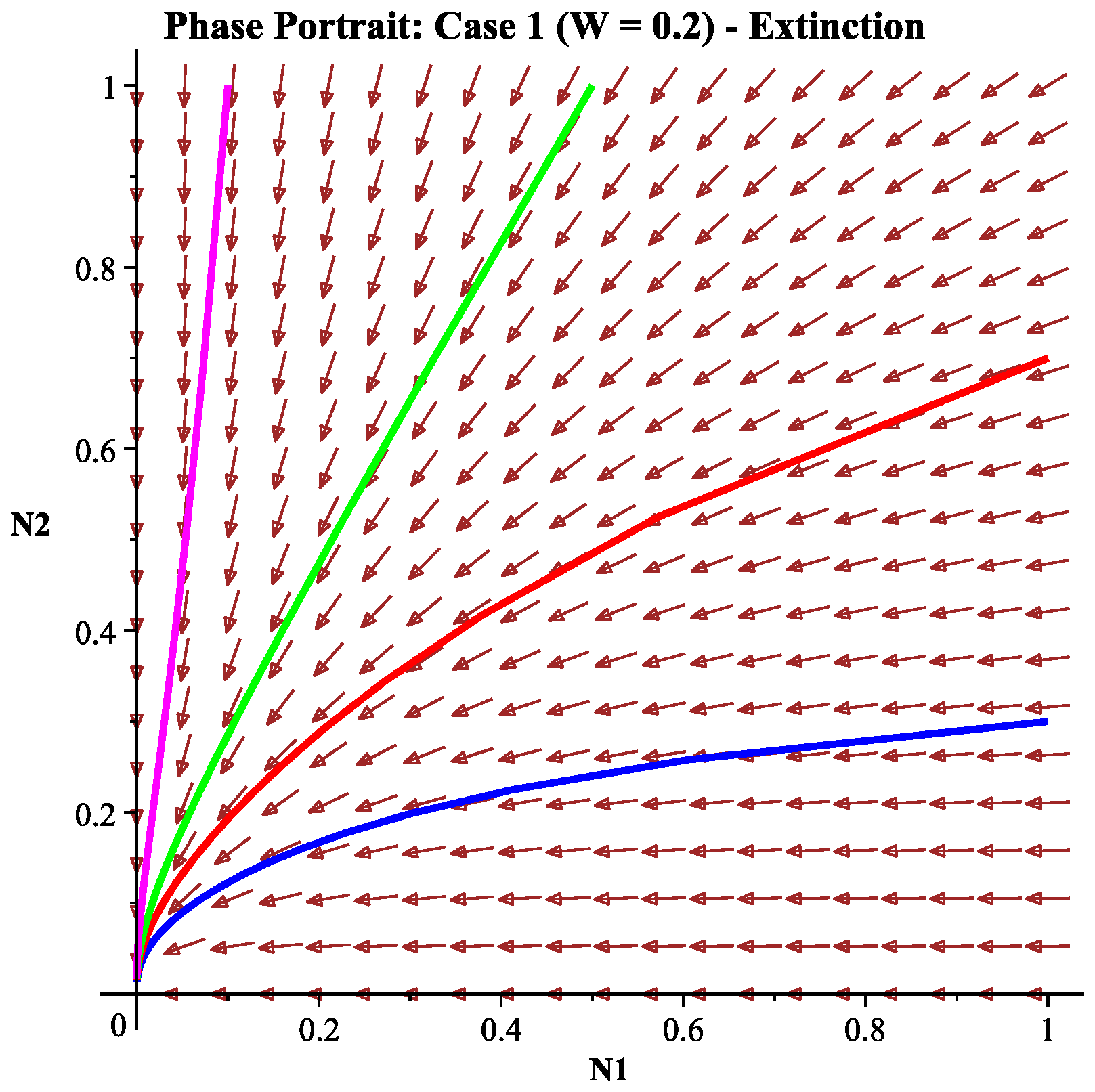
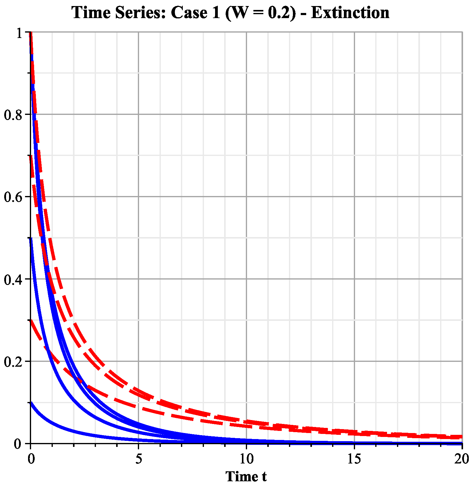
Numerical simulation results are shown in Figure 2 and Figure 3, selecting four different initial values ( N 1 ( 0 ) , N 2 ( 0 ) ) = ( 1 , 0.3 ) , ( 1 , 0.7 ) , ( 0.5 , 1 ) , ( 0.1 , 1 ) . All trajectories tend to the origin ( 0 , 0 ) .
  • Ecological interpretation: Under low-wind-speed conditions, the effective harvesting effort remains high, and the intrinsic growth rates of both species cannot overcome their harvesting mortality rates, leading the system to eventually approach the extinction of both species. This simulates the ecological disaster scenario of overharvesting.

6.2.2. Case 2: Medium Wind Speed Interval W 2 < W = 0.5 < W 1

When W = 0.5 ,
u ˜ ( 0.5 ) = 0.5 1 + 0.3 × 0.5 0.435 , E ˜ ( 0.5 ) = e 0.5 × 0.5 0.779 .
The equilibrium point calculation is as follows:
  • N 20 = 1 × 1 1.5 × 0.779 × 0.8 1.0 0.065 ( E 2 exists).
  • N 10 = 1 × 1 1.8 × 0.779 × 0.8 1.0 0.122 ( E 1 does not exist since N 10 < 0 ).
Since W 2 < W < W 1 , species 2 already meets the survival condition, while species 1 does not yet. According to the global stability theorem (Theorem 12), E 2 = ( 0 , 0.065 ) is globally stable.
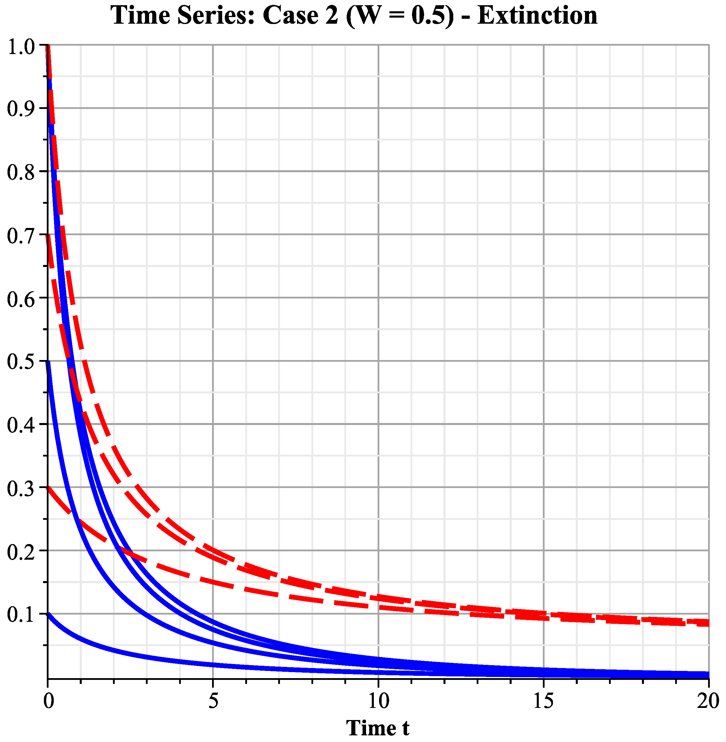
Numerical simulation results are shown in Figure 4 and Figure 5, where trajectories under different initial conditions all tend to ( 0 , 0.065 ) .
  • Ecological interpretation: The increase in wind speed reduces harvesting effort, allowing species 2 (with catchability coefficient q 2 = 1.5 less than species 1’s q 1 = 1.8 ), which is relatively less vulnerable to harvesting, to first break through the survival threshold, survive, and establish a population. Species 1, suffering greater harvesting pressure, still becomes extinct. The system is in the state of species 2 exclusivity, perfectly verifying that under the W 2 < W 1 scenario, the system first enters this intermediate transition phase as wind speed increases.

6.2.3. Case 3: Intermediate Wind Speed Interval W 1 < W = 0.8 < W 3

At a wind speed of W = 0.8 , which lies between the critical values W 1 0.588 and W 3 0.932 , the system parameters become
u ^ ( 0.8 ) = 0.5 1 + 0.3 × 0.8 0.403 , E ^ ( 0.8 ) = e 0.5 × 0.8 0.670 .
The equilibrium analysis reveals three possible steady states. The boundary equilibrium E 2 , representing exclusive survival of species 2, occurs at
N 20 = 1 1.5 × 0.670 × 0.8 1.0 0.196 .
Similarly, the boundary equilibrium E 1 for species 1 exclusivity is found at
N 10 = 1 1.8 × 0.670 × 0.8 1.0 0.035 .
However, the positive coexistence equilibrium E * yields
N 1 * = 0.035 0.403 × 0.196 0.044 ,
indicating that the coexistence state is ecologically infeasible in this wind regime.
Stability analysis confirms that while both boundary equilibria E 1 and E 2 exist, only E 2 is asymptotically stable. The trivial equilibrium E 0 is unstable due to reduced harvesting pressure, and E 1 functions as a saddle point. These results align with Theorem 12, establishing E 2 as globally asymptotically stable throughout the domain Ω .
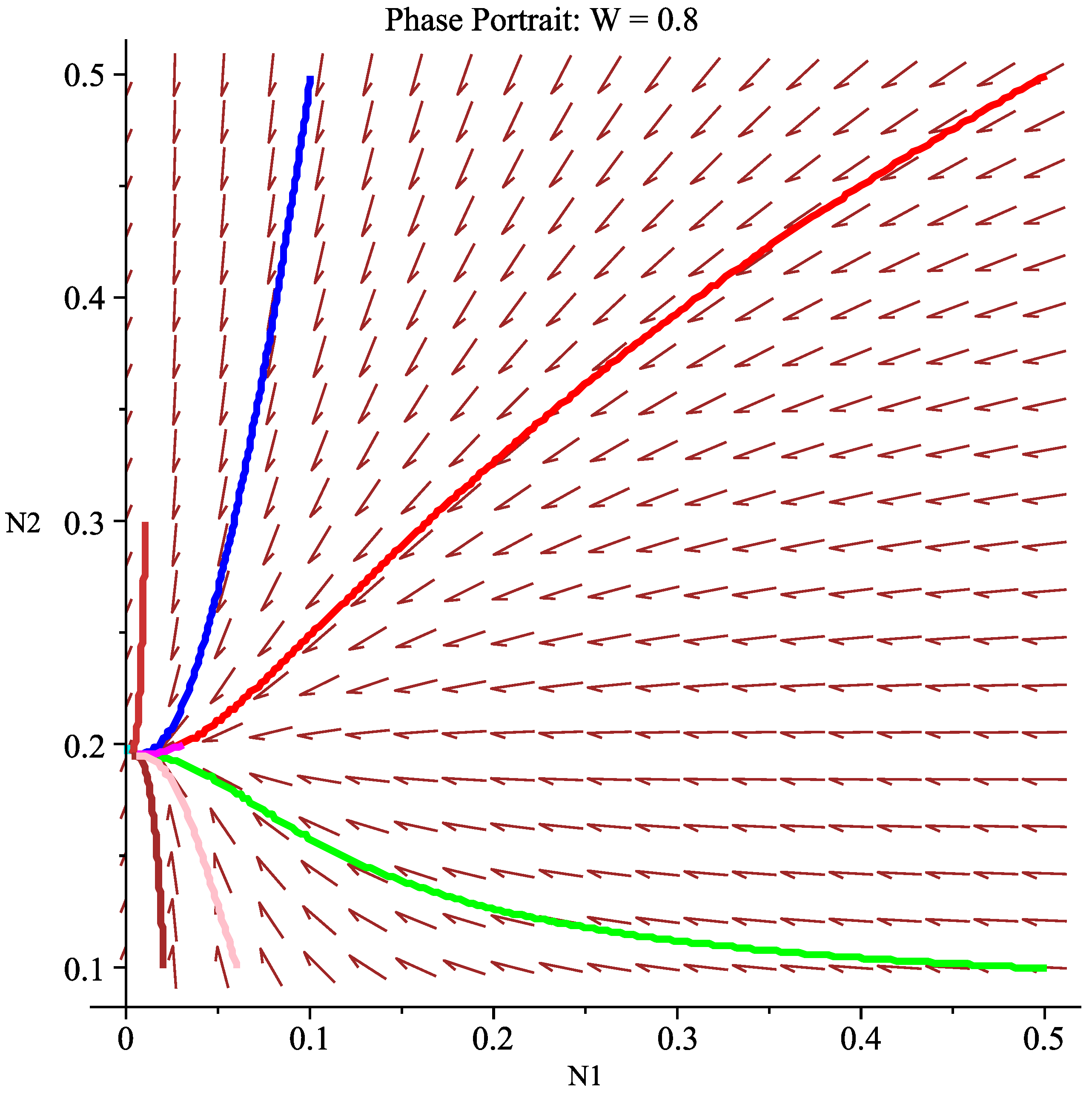
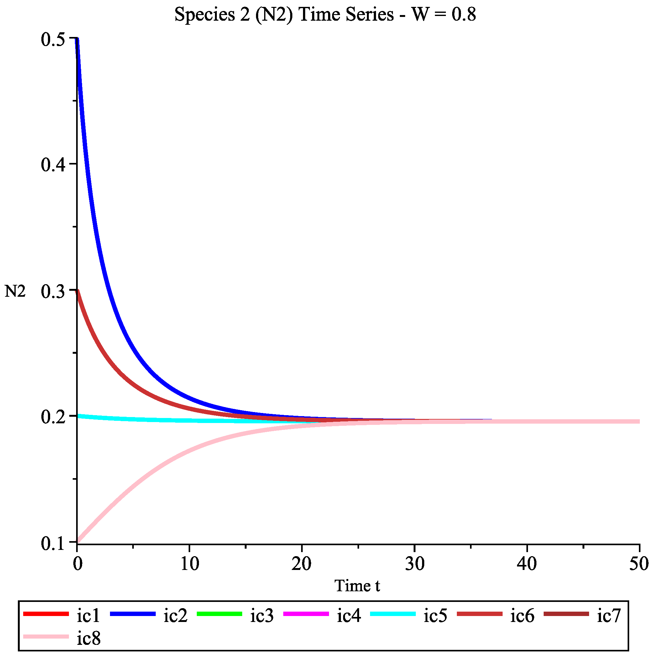
Numerical simulations validate these theoretical predictions. The phase portrait (Figure 6) demonstrates global convergence to E 2 = ( 0 , 0.196 ) from diverse initial conditions (0.5, 0.5), (0.1, 0.5), (0.5, 0.1), (0.03, 0.2), (0.02, 0.2), (0.01, 0.3), (0.02, 0.1), and (0.06, 0.1). Time series analysis further elucidates this dynamic: species 1 populations invariably decline to extinction (Figure 7), while species 2 densities stabilize at approximately 0.196 (Figure 8) regardless of initial population sizes.
  • Ecological interpretation: Ecologically, this intermediate wind regime represents a critical transition phase. Although species 1 possesses sufficient growth rate to overcome harvesting pressure in isolation ( r 1 > q 1 E ˜ m ), the persistent amensalistic effect from species 2 ( u ˜ 0.403 ) prevents stable coexistence. The system therefore converges to exclusive dominance by species 2, confirming the theoretical framework established in Section 4.5 for the parameter regime where W 2 < W 1 < W < W 3 .

6.2.4. Case 4: High Wind Speed Interval W = 3.0 > W 3

When W = 3.0 ,
u ˜ ( 3.0 ) = 0.5 1 + 0.3 × 3.0 0.263 , E ˜ ( 3.0 ) = e 0.5 × 3.0 0.223 .
The equilibrium point calculation is as follows:
N 20 = 1 × 1 1.5 × 0.223 × 0.8 1.0 0.732 ,
N 1 * = 1 × 1 1.8 × 0.223 × 0.8 1.0 0.263 × 1 1.5 × 0.223 × 0.8 1.0 = 1 0.3213 0.263 × 0.7322 0.6787 0.1926 = 0.4861 .
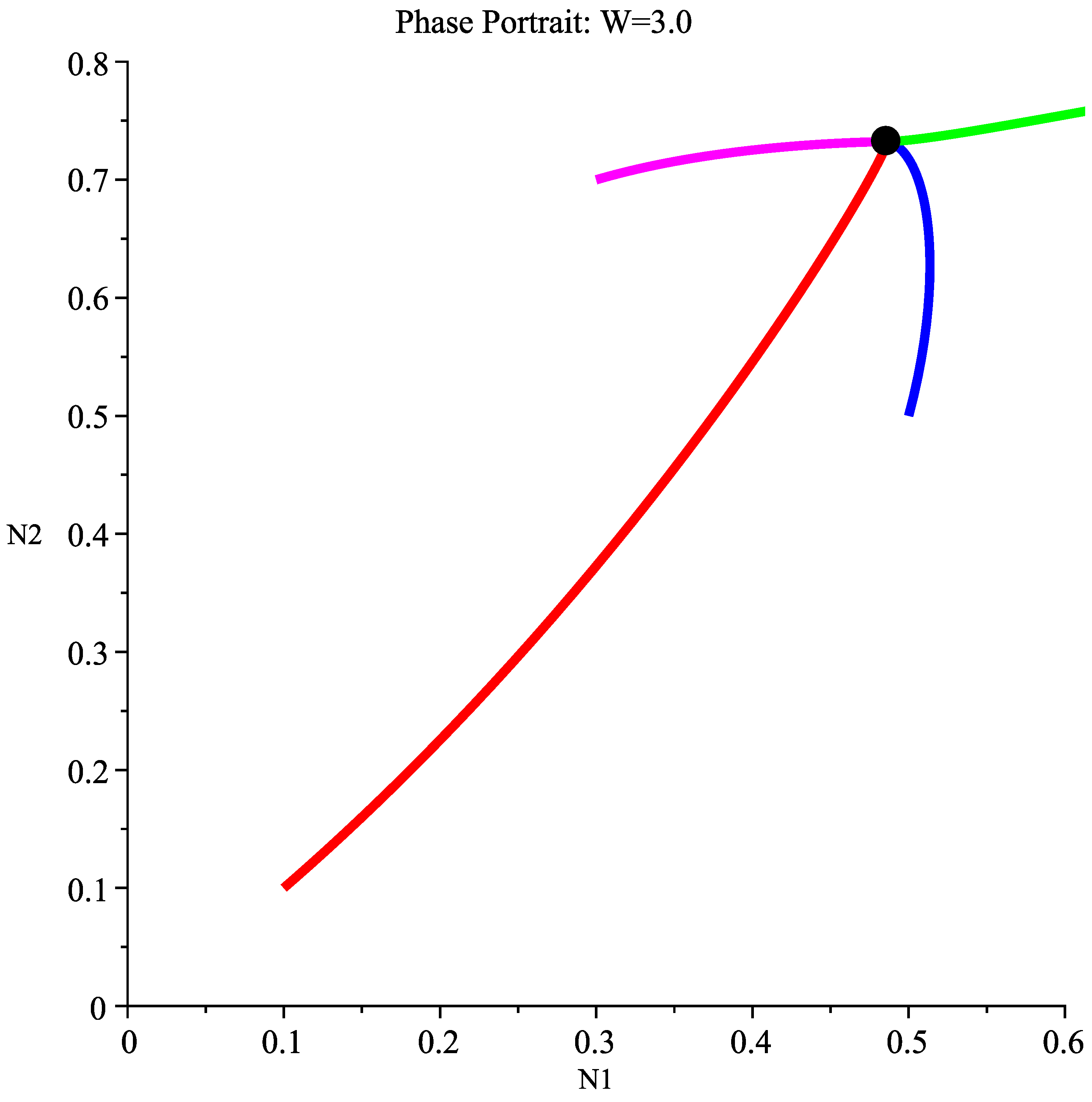
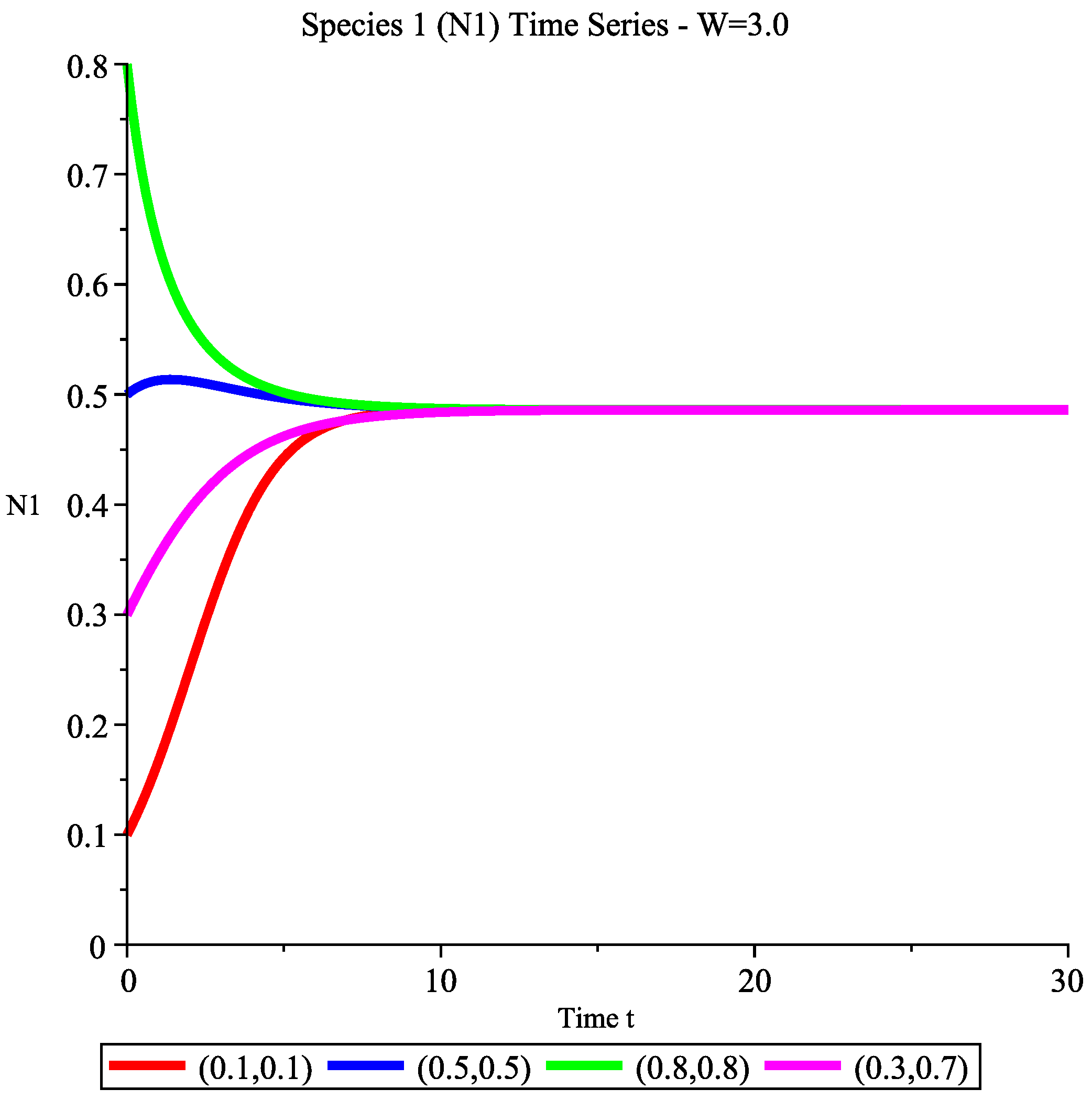
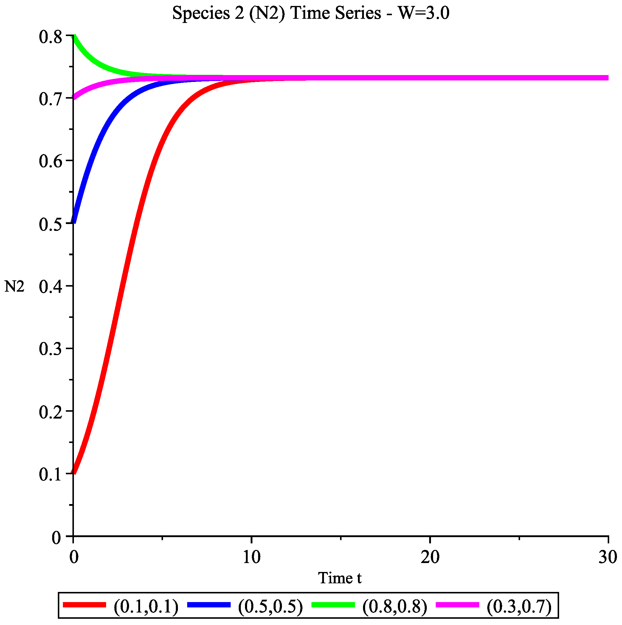
At this point, the positive equilibrium point E * = ( 0.486 , 0.732 ) exists and is globally stable.
Numerical simulation results are shown in Figure 9, Figure 10 and Figure 11, where trajectories under different initial conditions (0.1, 0.1), (0.5, 0.5), (0.8, 0.8), and (0.3, 0.7) all tend to the stable coexistence point (0.486, 0.732).
Ecological interpretation: Under high-wind-speed conditions, harvesting effort significantly decreases, while wind mixing greatly weakens the amensalistic effect of species 2 on species 1. This dual positive effect allows the population density of species 1 to increase substantially, and both species achieve stable coexistence at a higher level.

6.3. Management Implications and Discussion

Within the context of our hypothetical temperate coastal fishery, the proposed concept translates into a directly applicable quantitative basis for management. The critical wind speed W 3 0.93 m/s, for instance, provides a specific target. If empirical studies in a real system analogous to our scenario confirmed a similar threshold, managers could trigger effort reductions when forecasts predict sustained winds below this value to prevent the collapse of the valuable species 1.
The numerical simulation results provide important ecological management implications:
1.
Identification and application of critical wind speeds: For specific sea areas, the critical wind speed W 3 for ecological recovery can be determined by estimating model parameters. When forecasted wind speeds are consistently below W 3 , fishery management alerts should be triggered.
2.
Adaptive harvesting management: During low-wind-speed seasons ( W < W 3 ), fishery management departments should proactively reduce harvesting effort (e.g., decrease fishing vessel operation days) to simulate the ecological effects of high wind speeds and assist population recovery.
3.
Marine protected area planning: When formulating marine protected area plans, priority should be given to sea areas with favorable wind conditions (i.e., higher average wind speeds) or areas located in wind channels, utilizing natural wind power to promote biodiversity within protected areas.
4.
Wind as an ecological restoration tool: This study theoretically demonstrates that wind is a natural force that can promote ecological recovery. When conditions permit, even artificial interventions to enhance local mixing (simulating wind effects) could be considered as auxiliary means for restoring degraded ecosystems.
Remark 1.
We received the following review comments: “Even if the authors used hypothetical parameter values, it would be beneficial to compare their threshold wind speed values with those reported in the literature as strong enough to affect fishing activity or harvesting effort, as this comparison would help substantiate their discussion. Without such justification, it remains difficult to agree with the authors’ statements on management implications in Section 6.3.” The study by Hansen et al. [72] indicates that since 1971, there has been an annual decrease in the number of days with wind conditions suitable for safely hunting bowhead whales and caribou. The window of hunting opportunity has been reduced by up to seven days. Wind speed thresholds of 6 m/s and 11 m/s were identified, beyond which hunting becomes entirely unfeasible due to excessively high winds. Although these specific thresholds appear to differ considerably from those in our study, the fundamental concept of observing and defining thresholds aligns with our theoretical research. This suggests that our results may have potential practical value.

7. Discussion and Conclusions

This study has developed a theoretical framework that positions wind speed as a central determinant in the dynamics of harvested amensalism systems. By integrating wind as a core parameter rather than an external disturbance, the model reveals how environmental factors can systematically alter ecosystem stability through dual regulatory pathways. The analysis demonstrates that wind-driven transitions between extinction, exclusion, and coexistence states are not merely possible but predictable, governed by the interplay between anthropogenic pressure and biological interactions.
The theoretical insights from this work carry significant implications for ecosystem-based management. The identification of critical wind speeds, particularly the coexistence threshold W 3 , provides a quantitative basis for adaptive fisheries management. In practical terms, this suggests that fisheries managing systems where amensal relationships are suspected could benefit from incorporating wind forecasts into management decisions. During extended periods of calm weather ( W < W 3 ), preemptive effort reductions could prevent the system from crossing ecological thresholds that would be difficult to reverse. This approach aligns with emerging paradigms in predictive ecology that seek to anticipate regime shifts rather than merely responding to them.
Furthermore, the model provides a mechanistic explanation for why certain marine protected areas (MPAs) might outperform others. The theoretical preference for windier regions emerges naturally from the dual effect of wind on both harvesting efficiency and amensalism intensity. This suggests that strategic MPA placement in well-mixed, wind-exposed regions could leverage natural conditions to enhance conservation outcomes, creating more effective refuges that naturally experience reduced stress on multiple fronts.
The framework also offers a new lens for diagnosing puzzling ecosystem behaviors. The persistent decline of a species despite reduced fishing pressure—a phenomenon observed in several managed fisheries—could be reinterpreted through the model’s logic. Such patterns may indicate the presence of previously unquantified biological interactions, such as amensalism, that maintain suppression even as direct anthropogenic pressure diminishes. This highlights the critical importance of understanding species interaction networks for effective ecosystem management.
Three fundamental conclusions emerge from this research. First, environmental drivers like wind can function as decisive ecological regulators, capable of overriding the destabilizing effects of both harvesting and asymmetric species interactions. Second, stable coexistence emerges through the simultaneous mitigation of multiple stressors—in this case, the dual reduction of harvesting mortality and amensalism intensity. Third, the concept of critical wind speeds transforms abstract stability thresholds into potential management tools, enabling a shift from reactive to predictive approaches in ecosystem management.
In summary, this research establishes that the pathway to sustainable coexistence in anthropogenically stressed ecosystems may be found not only in direct management interventions but also in harnessing environmental forces that naturally promote biodiversity. By rigorously characterizing the wind-driven dynamics of a harvested amensalism system, we provide both a theoretical foundation and a quantitative framework for designing management strategies that work with, rather than against, natural environmental processes.
At the end of this paper, we are deeply grateful to the three reviewers for their meticulous review and invaluable suggestions, which have been instrumental in enhancing the quality of this work.

Author Contributions

Writing—original draft preparation, Q.Y., T.B., and F.C.; writing—review and editing, Q.Y., T.B., and F.C. All authors have read and agreed to the published version of the manuscript.

Funding

This research was funded by the Anhui Provincial Research Center for Eco-agriculture of Chinese Medicinal Herbs Research Platform Project; 2024 school-level Scientific Research Project (Research on Population Characteristics of Wild Dendrobium huoshanense Based on Biodynamic Model); school-level Quality Engineering Project (wxxy2024115) and the Natural Science Foundation of Fujian Province (2024J01273), the Special Research Innovation Platform Project of the Data Intelligence and Dabie Mountains Rural Revitalization Key Laboratory of Philosophy and Social Sciences in Anhui Province (WXSK202321) and The Open Fund ofAnhui Provincial Key Laboratory of Philosophy and Social Sciences for Data Intelligence and Rural Revitalization of Dabie Mountains (Grant No. WXSK202321).

Data Availability Statement

No new data were created or analyzed in this study.

Conflicts of Interest

The authors declare no conflicts of interest.

Appendix A

Proof of Theorem 1. 
Substitute N 1 = 0 , N 2 = 0 into system (5):
f 1 ( 0 , 0 ) = r 1 · 0 · 1 0 P 1 u ˜ P 1 · 0 q 1 E ˜ m · 0 = 0 ,
f 2 ( 0 , 0 ) = r 2 · 0 · 1 0 P 2 q 2 E ˜ m · 0 = 0 .
Therefore, E 0 = ( 0 , 0 ) is an equilibrium point of the system. This ends the proof of Theorem 1. □

Appendix B

Proof of Theorem 2. 
Set N 2 = 0 and substitute into the equilibrium condition (6):
f 1 ( N 1 , 0 ) = r 1 N 1 1 N 1 P 1 q 1 E ˜ m N 1 = 0 ,
f 2 ( N 1 , 0 ) = 0 ( automatically satisfied ) .
For N 1 0 , we have
r 1 1 N 1 P 1 q 1 E ˜ m = 0 .
Solving for N 1 ,
N 1 = P 1 1 q 1 E ˜ m r 1 = N 10 .
For N 10 > 0 , the following condition must be satisfied:
1 q 1 E ˜ m r 1 > 0 r 1 > q 1 E ˜ m .
Therefore, the positive boundary equilibrium point E 1 = ( N 10 , 0 ) exists if and only if condition (7) holds. We have thus proved Theorem 2. □

Appendix C

Proof of Theorem 3. 
Set N 1 = 0 and substitute into the equilibrium condition (6):
f 1 ( 0 , N 2 ) = 0 ( automatically satisfied ) ,
f 2 ( 0 , N 2 ) = r 2 N 2 1 N 2 P 2 q 2 E ˜ m N 2 = 0 .
For N 2 0 , we have
r 2 1 N 2 P 2 q 2 E ˜ m = 0 .
Solving for N 2 ,
N 2 = P 2 1 q 2 E ˜ m r 2 = N 20 .
For N 20 > 0 , the following condition must be satisfied:
1 q 2 E ˜ m r 2 > 0 r 2 > q 2 E ˜ m .
Therefore, the positive boundary equilibrium point E 2 = ( 0 , N 20 ) exists if and only if condition (9) holds. □

Appendix D

Proof of Theorem 4. 
Assume N 1 > 0 , N 2 > 0 . From the equilibrium condition (6), we obtain
r 1 1 N 1 P 1 u ˜ P 1 N 2 q 1 E ˜ m = 0 , r 2 1 N 2 P 2 q 2 E ˜ m = 0 .
From the second equation of (A1), solve for N 2 :
1 N 2 P 2 = q 2 E ˜ m r 2 N 2 = P 2 1 q 2 E ˜ m r 2 = N 2 * .
For N 2 * > 0 , the following condition must be satisfied:
1 q 2 E ˜ m r 2 > 0 r 2 > q 2 E ˜ m .
Substitute N 2 * into the first equation of (A1),
r 1 1 N 1 P 1 u ˜ P 1 P 2 1 q 2 E ˜ m r 2 q 1 E ˜ m = 0 .
Rearranging gives
1 N 1 P 1 = q 1 E ˜ m r 1 + u ˜ P 2 P 1 1 q 2 E ˜ m r 2 .
Solving for N 1 :
N 1 = P 1 1 q 1 E ˜ m r 1 u ˜ P 2 P 1 1 q 2 E ˜ m r 2 = def N 1 * .
For N 1 * > 0 , the following condition must be satisfied:
1 q 1 E ˜ m r 1 u ˜ P 2 P 1 1 q 2 E ˜ m r 2 > 0 .
Therefore, the positive equilibrium point E * = ( N 1 * , N 2 * ) exists if and only if both conditions above are simultaneously satisfied. □

Appendix E

Proof of Theorem 5. 
Compute the Jacobian matrix at E 0 = ( 0 , 0 ) :
J ( 0 , 0 ) = r 1 q 1 E ˜ m 0 0 r 2 q 2 E ˜ m .
This is a diagonal matrix, and its eigenvalues are the diagonal elements:
λ 1 = r 1 q 1 E ˜ m , λ 2 = r 2 q 2 E ˜ m .
Analyze stability based on the signs of eigenvalues:
  • If λ 1 < 0 and λ 2 < 0 , i.e., r 1 < q 1 E ˜ m and r 2 < q 2 E ˜ m , then E 0 is a stable node;
  • If λ 1 > 0 or λ 2 > 0 , i.e., r 1 > q 1 E ˜ m or r 2 > q 2 E ˜ m , then E 0 is an unstable node.

Appendix F

Proof of Theorem 6. 
Compute the elements of the Jacobian matrix at E 1 = ( N 10 , 0 ) . First, compute
f 1 N 1 | E 1 = r 1 2 r 1 N 10 P 1 q 1 E ˜ m .
Using the equilibrium condition satisfied by E 1 ,
r 1 1 N 10 P 1 q 1 E ˜ m = 0 1 N 10 P 1 = q 1 E ˜ m r 1 ,
Substitute to get
f 1 N 1 | E 1 = r 1 2 r 1 N 10 P 1 q 1 E ˜ m = r 1 r 1 N 10 P 1 q 1 E ˜ m r 1 N 10 P 1 = 0 r 1 N 10 P 1 = r 1 N 10 P 1 .
Other partial derivatives are as follows:
f 1 N 2 | E 1 = r 1 u ˜ P 1 N 10 , f 2 N 1 | E 1 = 0 , f 2 N 2 | E 1 = r 2 q 2 E ˜ m .
Therefore, the Jacobian matrix at E 1 is
J ( N 10 , 0 ) = r 1 N 10 P 1 r 1 u ˜ P 1 N 10 0 r 2 q 2 E ˜ m .
This is an upper triangular matrix, and its eigenvalues are the diagonal elements:
λ 1 = r 1 N 10 P 1 < 0 , λ 2 = r 2 q 2 E ˜ m .
The stability analysis is as follows:
  • If λ 2 < 0 , i.e., r 2 < q 2 E ˜ m , then both eigenvalues are negative, and E 1 is a stable node;
  • If λ 2 > 0 , i.e., r 2 > q 2 E ˜ m , then one eigenvalue is negative and one positive, and E 1 is a saddle point (unstable).

Appendix G

Proof of Theorem 7. 
Compute the elements of the Jacobian matrix at E 2 = ( 0 , N 20 ) . First, compute
f 1 N 1 | E 2 = r 1 r 1 u ˜ P 1 N 20 q 1 E ˜ m = r 1 1 u ˜ N 20 P 1 q 1 E ˜ m .
Other partial derivatives are as follows:
f 1 N 2 | E 2 = 0 , f 2 N 1 | E 2 = 0 , f 2 N 2 | E 2 = r 2 2 r 2 N 20 P 2 q 2 E ˜ m .
Using the equilibrium condition satisfied by E 2 ,
r 2 1 N 20 P 2 q 2 E ˜ m = 0 1 N 20 P 2 = q 2 E ˜ m r 2 ,
Substitute to get
f 2 N 2 | E 2 = r 2 2 r 2 N 20 P 2 q 2 E ˜ m = r 2 r 2 N 20 P 2 q 2 E ˜ m r 2 N 20 P 2 = 0 r 2 N 20 P 2 = r 2 N 20 P 2 .
Therefore, the Jacobian matrix at E 2 is
J ( 0 , N 20 ) = r 1 1 u ˜ N 20 P 1 q 1 E ˜ m 0 0 r 2 N 20 P 2 .
This is a diagonal matrix, and its eigenvalues are
λ 1 = r 1 1 u ˜ N 20 P 1 q 1 E ˜ m , λ 2 = r 2 N 20 P 2 < 0 .
The stability analysis is as follows:
  • If λ 1 < 0 , i.e., r 1 1 u ˜ N 20 P 1 < q 1 E ˜ m , then both eigenvalues are negative, and E 2 is a stable node;
  • If λ 1 > 0 , i.e., r 1 1 u ˜ N 20 P 1 > q 1 E ˜ m , then one eigenvalue is positive and one negative, and E 2 is a saddle point (unstable).

Appendix H

Proof of Theorem 8. 
Compute the elements of the Jacobian matrix at E * = ( N 1 * , N 2 * ) . First, compute
f 1 N 1 | E * = r 1 2 r 1 N 1 * P 1 r 1 u ˜ P 1 N 2 * q 1 E ˜ m .
Using the equilibrium conditions satisfied by E * ,
r 1 1 N 1 * P 1 u ˜ P 1 N 2 * q 1 E ˜ m = 0 , r 2 1 N 2 * P 2 q 2 E ˜ m = 0 ,
Substitute to get
f 1 N 1 | E * = r 1 2 r 1 N 1 * P 1 r 1 u ˜ P 1 N 2 * q 1 E ˜ m = r 1 r 1 N 1 * P 1 r 1 u ˜ P 1 N 2 * q 1 E ˜ m r 1 N 1 * P 1 = 0 r 1 N 1 * P 1 = r 1 N 1 * P 1 .
Other partial derivatives are as follows:
f 1 N 2 | E * = r 1 u ˜ P 1 N 1 * , f 2 N 1 | E * = 0 , f 2 N 2 | E * = r 2 2 r 2 N 2 * P 2 q 2 E ˜ m = r 2 N 2 * P 2 .
Therefore, the Jacobian matrix at E * is
J ( N 1 * , N 2 * ) = r 1 N 1 * P 1 r 1 u ˜ P 1 N 1 * 0 r 2 N 2 * P 2 .
This is an upper triangular matrix, and its eigenvalues are the diagonal elements:
λ 1 = r 1 N 1 * P 1 < 0 , λ 2 = r 2 N 2 * P 2 < 0 .
Since N 1 * > 0 , N 2 * > 0 , and all parameters are positive, we have λ 1 < 0 , λ 2 < 0 . Both eigenvalues are negative real numbers; therefore, E * is a locally asymptotically stable node. □

Appendix I

Proof of Theorem 9. 
Consider the dynamics of species 1:
d N 1 d t = r 1 N 1 1 N 1 P 1 u ˜ P 1 N 2 q 1 E ˜ m N 1 r 1 N 1 1 N 1 P 1 .
This is an upper bound of the logistic growth equation. When N 1 > P 1 , d N 1 d t < 0 ; therefore, N 1 ( t ) cannot exceed P 1 . Similarly, for species 2,
d N 2 d t = r 2 N 2 1 N 2 P 2 q 2 E ˜ m N 2 r 2 N 2 1 N 2 P 2 ,
therefore, N 2 ( t ) cannot exceed P 2 . Hence, the system solutions are uniformly bounded. □

Appendix J

Proof of Theorem 10. 
Construct the Lyapunov function:
V 0 ( N 1 , N 2 ) = N 1 + N 2 .
Clearly, V 0 satisfies the following:
1.
V 0 ( 0 , 0 ) = 0 ;
2.
For any ( N 1 , N 2 ) Ω { ( 0 , 0 ) } , V 0 ( N 1 , N 2 ) > 0 ;
3.
V 0 is radially unbounded.
Calculate the time derivative of V 0 along system trajectories:
d V 0 d t = d N 1 d t + d N 2 d t = r 1 N 1 1 N 1 P 1 u ˜ P 1 N 2 q 1 E ˜ m N 1 + r 2 N 2 1 N 2 P 2 q 2 E ˜ m N 2 .
Expanding and recombining terms,
d V 0 d t = r 1 N 1 r 1 P 1 N 1 2 r 1 u ˜ P 1 N 1 N 2 q 1 E ˜ m N 1 + r 2 N 2 r 2 P 2 N 2 2 q 2 E ˜ m N 2 = ( r 1 q 1 E ˜ m ) N 1 + ( r 2 q 2 E ˜ m ) N 2 r 1 P 1 N 1 2 r 2 P 2 N 2 2 r 1 u ˜ P 1 N 1 N 2 .
Under condition (16), we have
( r 1 q 1 E ˜ m ) N 1 0 , ( r 2 q 2 E ˜ m ) N 2 0 .
Since all parameters are positive, we have
r 1 P 1 N 1 2 0 , r 2 P 2 N 2 2 0 , r 1 u ˜ P 1 N 1 N 2 0 .
Therefore,
d V 0 d t r 1 P 1 N 1 2 r 2 P 2 N 2 2 0 .
Now analyze the condition for equality. Suppose d V 0 d t = 0 ; then from (A25), we get
r 1 P 1 N 1 2 r 2 P 2 N 2 2 = 0 N 1 = 0 and N 2 = 0 .
Conversely, when N 1 = N 2 = 0 , clearly d V 0 d t = 0 .
Therefore, d V 0 d t = 0 if and only if ( N 1 , N 2 ) = ( 0 , 0 ) .
According to the Lyapunov global stability theorem, E 0 is globally asymptotically stable in Ω . □

Appendix K

Proof of Theorem 11. 
We employ the classical Volterra-type Lyapunov function for rigorous proof.
Define the function:
V ( N 1 , N 2 ) = η N 1 N 10 N 10 ln N 1 N 10 + N 2 ,
where η > 0 is an undetermined positive constant whose specific value will be determined later to ensure the derivative of the Lyapunov function is negative.
This function satisfies the following in domain Ω :
  • V ( N 10 , 0 ) = 0 ;
  • For any ( N 1 , N 2 ) ( N 10 , 0 ) , since the function x a a ln x a 0 (equality holds if and only if x = a ), and N 2 0 , we have V ( N 1 , N 2 ) > 0 ;
  • V is radially unbounded, i.e., when ( N 1 , N 2 ) , V ( N 1 , N 2 ) .
Calculate the total derivative of V along system trajectories:
d V d t = η 1 N 10 N 1 f 1 ( N 1 , N 2 ) + f 2 ( N 1 , N 2 ) .
At the equilibrium point E 1 = ( N 10 , 0 ) , we have f 1 ( N 10 , 0 ) = 0 , i.e.,
r 1 N 10 1 N 10 P 1 q 1 E ˜ m N 10 = 0 .
Since N 10 > 0 , we obtain
r 1 1 N 10 P 1 q 1 E ˜ m = 0 1 N 10 P 1 = q 1 E ˜ m r 1 .
Using Equation (A27), rewrite f 1 as
f 1 = r 1 N 1 1 N 1 P 1 u ˜ P 1 N 2 q 1 E ˜ m N 1 = r 1 N 1 1 N 1 P 1 u ˜ P 1 N 2 1 N 10 P 1 = r 1 N 1 N 10 N 1 P 1 u ˜ P 1 N 2 .
Substitute Equation (A28) into Equation (A26):
d V d t = η 1 N 10 N 1 · r 1 N 1 N 10 N 1 P 1 u ˜ P 1 N 2 + f 2 ( N 1 , N 2 ) = η r 1 P 1 ( N 1 N 10 ) 2 η r 1 u ˜ P 1 ( N 1 N 10 ) N 2 + f 2 ( N 1 , N 2 ) .
For f 2 ( N 1 , N 2 ) , under the condition r 2 q 2 E ˜ m , we have
f 2 ( N 1 , N 2 ) = r 2 N 2 1 N 2 P 2 q 2 E ˜ m N 2 r 2 P 2 N 2 2 .
Substitute (A30) into (A29), and let x = N 1 N 10 , y = N 2 , yielding
d V d t η r 1 P 1 x 2 η r 1 u ˜ P 1 x y r 2 P 2 y 2 .
Define the quadratic form Q ( x , y ) :
Q ( x , y ) = η r 1 P 1 x 2 + η r 1 u ˜ P 1 x y + r 2 P 2 y 2 .
Then Equation (A31) can be written as
d V d t Q ( x , y ) .
The symmetric matrix corresponding to the quadratic form Q ( x , y ) is
M = η r 1 P 1 η r 1 u ˜ 2 P 1 η r 1 u ˜ 2 P 1 r 2 P 2 .
The necessary and sufficient conditions for matrix M to be positive definite are
1.
η r 1 P 1 > 0 (obviously holds);
2.
det ( M ) > 0 .
Calculate the determinant:
det ( M ) = η r 1 P 1 r 2 P 2 η r 1 u ˜ 2 P 1 2 = η r 1 r 2 P 1 P 2 η 2 r 1 2 u ˜ 2 4 P 1 2 .
Set det ( M ) > 0 :
η r 1 r 2 P 1 P 2 > η 2 r 1 2 u ˜ 2 4 P 1 2 .
Multiply both sides by the positive number 4 P 1 2 r 1 :
4 η P 1 r 2 P 2 > η 2 r 1 u ˜ 2 .
Since η > 0 , we can solve for
η < 4 P 1 r 2 P 2 r 1 u ˜ 2 .
Therefore, as long as we select a positive constant η satisfying (A33), for example,
η = 2 P 1 r 2 P 2 r 1 u ˜ 2 ,
we can guarantee that matrix M is positive definite, and thus there exists a constant c > 0 such that
Q ( x , y ) c ( x 2 + y 2 ) = c ( N 1 N 10 ) 2 + N 2 2 .
Substitute (A34) into (A32):
d V d t c ( N 1 N 10 ) 2 + N 2 2 0 .
Equality holds if and only if N 1 = N 10 and N 2 = 0 , i.e., only at the equilibrium point E 1 .
According to the Lyapunov global asymptotic stability theorem and LaSalle’s invariance principle, within region Ω , all trajectories tend to E 1 as t . Therefore, the boundary equilibrium point E 1 is globally asymptotically stable in Ω . □

Appendix L

Proof of Theorem 12. 
Define the function:
V ( N 1 , N 2 ) = N 1 + η N 2 N 20 N 20 ln N 2 N 20 ,
where η > 0 is an undetermined positive constant, whose specific value will be determined later to ensure the derivative of the Lyapunov function is negative.
This function satisfies the following in domain Ω :
  • V ( 0 , N 20 ) = 0 ;
  • For any ( N 1 , N 2 ) ( 0 , N 20 ) , since the function y b b ln y b 0 (equality holds if and only if y = b ), and N 1 0 , we have V ( N 1 , N 2 ) > 0 ;
  • V is radially unbounded, i.e., when ( N 1 , N 2 ) , V ( N 1 , N 2 ) .
Calculate the total derivative of V along system trajectories:
d V d t = f 1 ( N 1 , N 2 ) + η 1 N 20 N 2 f 2 ( N 1 , N 2 ) .
At the equilibrium point E 2 = ( 0 , N 20 ) , we have f 2 ( 0 , N 20 ) = 0 , i.e.,
r 2 N 20 1 N 20 P 2 q 2 E ˜ m N 20 = 0 .
Since N 20 > 0 , we obtain
r 2 1 N 20 P 2 q 2 E ˜ m = 0 1 N 20 P 2 = q 2 E ˜ m r 2 .
Using Equation (A36), rewrite f 2 as
f 2 = r 2 N 2 1 N 2 P 2 q 2 E ˜ m N 2 = r 2 N 2 1 N 2 P 2 1 N 20 P 2 = r 2 N 2 N 20 N 2 P 2 .
Substitute Equation (A37) into Equation (A35):
d V d t = f 1 ( N 1 , N 2 ) + η 1 N 20 N 2 · r 2 N 2 N 20 N 2 P 2 = f 1 ( N 1 , N 2 ) η r 2 P 2 ( N 2 N 20 ) 2 .
Write f 1 as
f 1 = N 1 r 1 1 N 1 P 1 u ˜ P 1 N 2 q 1 E ˜ m .
To utilize the known conditions, we add and subtract r 1 1 u ˜ N 20 P 1 :
r 1 1 N 1 P 1 u ˜ P 1 N 2 q 1 E ˜ m = r 1 1 u ˜ N 20 P 1 q 1 E ˜ m + r 1 u ˜ N 20 P 1 N 1 P 1 u ˜ N 2 P 1 = r 1 1 u ˜ N 20 P 1 q 1 E ˜ m r 1 P 1 N 1 r 1 u ˜ P 1 ( N 2 N 20 ) .
From the theorem conditions
r 1 1 u ˜ N 20 P 1 q 1 E ˜ m 0 .
Substitute (A39) and (A40) into f 1 :
f 1 N 1 r 1 P 1 N 1 r 1 u ˜ P 1 ( N 2 N 20 ) = r 1 P 1 N 1 2 r 1 u ˜ P 1 N 1 ( N 2 N 20 ) .
Substitute (A41) into (A38):
d V d t r 1 P 1 N 1 2 r 1 u ˜ P 1 N 1 ( N 2 N 20 ) η r 2 P 2 ( N 2 N 20 ) 2 .
Let
x = N 1 , y = N 2 N 20 .
Then
d V d t r 1 P 1 x 2 r 1 u ˜ P 1 x y η r 2 P 2 y 2 .
Define the quadratic form:
Q ( x , y ) = r 1 P 1 x 2 + r 1 u ˜ P 1 x y + η r 2 P 2 y 2 .
Then
d V d t Q ( x , y ) .
The symmetric matrix corresponding to Q ( x , y ) is
M = r 1 P 1 r 1 u ˜ 2 P 1 r 1 u ˜ 2 P 1 η r 2 P 2 .
The necessary and sufficient conditions for matrix M to be positive definite are
1.
r 1 P 1 > 0 (obviously holds);
2.
det ( M ) > 0 .
Calculate the determinant:
det ( M ) = r 1 P 1 η r 2 P 2 r 1 u ˜ 2 P 1 2 = η r 1 r 2 P 1 P 2 r 1 2 u ˜ 2 4 P 1 2 .
Set det ( M ) > 0 :
η r 1 r 2 P 1 P 2 > r 1 2 u ˜ 2 4 P 1 2 .
Multiply both sides by the positive number 4 P 1 2 r 1 :
4 η P 1 r 2 P 2 > r 1 u ˜ 2 .
Solve for
η > r 1 u ˜ 2 P 2 4 r 2 P 1 .
Therefore, select
η = r 1 u ˜ 2 P 2 2 r 2 P 1 ,
This value satisfies inequality (A45), thus ensuring matrix M is positive definite. Hence,
d V d t c N 1 2 + ( N 2 N 20 ) 2 0 .
Equality holds if and only if N 1 = 0 and N 2 = N 20 , i.e., only at the equilibrium point E 2 .
According to the Lyapunov global asymptotic stability theorem and LaSalle’s invariance principle, within region Ω , all trajectories tend to E 2 as t . Therefore, the boundary equilibrium point E 2 is globally asymptotically stable in Ω . □

Appendix M

Proof of Theorem 13. 
We construct a Lyapunov function of the following form:
V ( N 1 , N 2 ) = η 1 N 1 N 1 * N 1 * ln N 1 N 1 * + η 2 N 2 N 2 * N 2 * ln N 2 N 2 * ,
where η 1 , η 2 > 0 are undetermined constants.
  • V ( N 1 * , N 2 * ) = 0 ;
  • For any ( N 1 , N 2 ) ( N 1 * , N 2 * ) , since the function x a a ln x a 0 (equality holds if and only if x = a ), we have V ( N 1 , N 2 ) > 0 ;
  • V is radially unbounded.
This shows that V is positive definite.
Calculate the total derivative of V along system trajectories:
d V d t = η 1 1 N 1 * N 1 f 1 ( N 1 , N 2 ) + η 2 1 N 2 * N 2 f 2 ( N 1 , N 2 ) .
Using the equilibrium conditions of E * ,
r 1 1 N 1 * P 1 u ˜ P 1 N 2 * q 1 E ˜ m = 0 , r 2 1 N 2 * P 2 q 2 E ˜ m = 0 ,
Rewrite f 1 , f 2 as
f 1 = r 1 P 1 N 1 ( N 1 N 1 * ) r 1 u ˜ P 1 N 1 ( N 2 N 2 * ) , f 2 = r 2 P 2 N 2 ( N 2 N 2 * ) .
Substitute into d V d t :
d V d t = η 1 1 N 1 * N 1 r 1 P 1 N 1 ( N 1 N 1 * ) r 1 u ˜ P 1 N 1 ( N 2 N 2 * ) + η 2 1 N 2 * N 2 r 2 P 2 N 2 ( N 2 N 2 * ) = η 1 r 1 P 1 ( N 1 N 1 * ) 2 η 1 r 1 u ˜ P 1 ( N 1 N 1 * ) ( N 2 N 2 * ) η 2 r 2 P 2 ( N 2 N 2 * ) 2 .
Let x = N 1 N 1 * , y = N 2 N 2 * , then
d V d t = η 1 r 1 P 1 x 2 + η 1 r 1 u ˜ P 1 x y + η 2 r 2 P 2 y 2 .
Define the quadratic form:
Q ( x , y ) = η 1 r 1 P 1 x 2 + η 1 r 1 u ˜ P 1 x y + η 2 r 2 P 2 y 2 ,
then
d V d t = Q ( x , y ) .
The symmetric matrix corresponding to Q ( x , y ) is
M = η 1 r 1 P 1 η 1 r 1 u ˜ 2 P 1 η 1 r 1 u ˜ 2 P 1 η 2 r 2 P 2 .
The necessary and sufficient conditions for M to be positive definite are
1.
η 1 r 1 P 1 > 0 (obviously holds);
2.
det ( M ) > 0 .
Calculate the determinant:
det ( M ) = η 1 r 1 P 1 η 2 r 2 P 2 η 1 r 1 u ˜ 2 P 1 2 = η 1 η 2 r 1 r 2 P 1 P 2 η 1 2 r 1 2 u ˜ 2 4 P 1 2 .
Set det ( M ) > 0 :
η 1 η 2 r 1 r 2 P 1 P 2 > η 1 2 r 1 2 u ˜ 2 4 P 1 2 η 2 > η 1 r 1 u ˜ 2 P 2 4 r 2 P 1 .
Therefore, we can choose
η 1 = 1 , η 2 = r 1 u ˜ 2 P 2 2 r 2 P 1 ,
then det ( M ) > 0 , and thus M is positive definite.
From this we know
d V d t 0 ,
with equality if and only if x = 0 , y = 0 , i.e., N 1 = N 1 * , N 2 = N 2 * .
By the Lyapunov global asymptotic stability theorem and LaSalle’s invariance principle, E * is globally asymptotically stable in Ω .

References

  1. Xi, X.; Griffin, J.N.; Sun, S. Grasshoppers amensalistically suppress caterpillar performance and enhance plant biomass in an alpine meadow. Oikos 2013, 122, 1049–1057. [Google Scholar] [CrossRef]
  2. Akimoto, S. Coexistence and weak amensalism of congeneric gall-forming aphids on the Japanese elm. Popul. Ecol. 1995, 37, 81–89. [Google Scholar] [CrossRef]
  3. Osakabe, M.; Hongo, K.; Funayama, K.; Osumi, S. Amensalism via webs causes unidirectional shifts of dominance in spider mite communities. Oecologia 2006, 150, 496–505. [Google Scholar] [CrossRef]
  4. Pommier, S.; Strehaiano, P.; Delia, M.L. Modelling the growth dynamics of interacting mixed cultures: A case of amensalism. Int. J. Food Microbiol. 2005, 100, 131–139. [Google Scholar] [CrossRef]
  5. Townsend, H.M.; Huyvaert, K.P.; Hodum, P.J.; Anderson, D.J. Nesting distributions of Galapagos boobies (Aves: Sulidae): An apparent case of amensalism. Oecologia 2002, 132, 419–427. [Google Scholar] [CrossRef]
  6. Xu, P. Dynamics of microbial competition, commensalism, and cooperation and its implications for coculture and microbiome engineering. Biotechnol. Bioeng. 2021, 118, 199–209. [Google Scholar] [CrossRef] [PubMed]
  7. Dairain, A.; Gonzalez, P.; Legeay, A.; Maire, O.; Daffe, G.; Pascal, L.; de Montaudouin, X. Parasite interactions in the bioturbator Upogebia pusilla (Decapoda: Gebiidae): A case of amensalism? Mar. Biol. 2017, 164, 203. [Google Scholar] [CrossRef]
  8. García, C.; Rendueles, M.; Diaz, M. Microbial amensalism in Lactobacillus casei and Pseudomonas taetrolens mixed culture. Bioprocess Biosyst. Eng. 2017, 40, 1111–1122. [Google Scholar] [CrossRef] [PubMed]
  9. Xiong, X.H.; Wang, B.B.; Zhang, H.L. Stability analysis on the dynamic model of fish swarm amensalism. Adv. Appl. Math. 2016, 5, 255–261. [Google Scholar] [CrossRef]
  10. Chen, B.G. Dynamic behaviors of a non-selective harvesting Lotka-Volterra amensalism model incorporating partial closure for the populations. Adv. Differ. Equ. 2018, 2018, 272. [Google Scholar] [CrossRef]
  11. Guan, X.Y.; Chen, F.D. Dynamical analysis of a two species amensalism model with Beddington–DeAngelis functional response and Allee effect on the second species. Nonlinear Anal. Real World Appl. 2019, 48, 71–93. [Google Scholar] [CrossRef]
  12. Chong, Y.; Hou, Y.; Chen, S.; Chen, F. The influence of fear effect to the dynamic behaviors of Lotka-Volterra ammensalism model. Eng. Lett. 2024, 32, 1233–1242. [Google Scholar]
  13. Chong, Y.; Zhu, Q.; Li, Q.; Chen, F. Dynamic behaviors of a two species amensalism model with a second species dependent cover. Eng. Lett. 2024, 32, 1553–1561. [Google Scholar]
  14. Chong, Y.; Chen, F. Global stability, bifurcations and chaos control in a discrete amensalism model with cover and saturation effect. J. Appl. Anal. Comput. 2025, 15, 2977–3003. [Google Scholar] [CrossRef] [PubMed]
  15. Gomez, J.M.; González-Megías, A. Asymmetrical interactions between ungulates and phytophagous insects: Being different matters. Ecology 2002, 83, 203–211. [Google Scholar] [CrossRef]
  16. Abd Alhadi, A.R.S.; Naji, R.K. The contribution of amensalism and parasitism in the three-species ecological system’s dynamic. Commun. Math. Biol. Neurosci. 2024, 2024, 33. [Google Scholar]
  17. Abd Alhadi, A.R.S.; Naji, R.K. The role of amensalism and parasitism on the dynamics of three species ecological system. Results Control Optim. 2025, 19, 100571. [Google Scholar] [CrossRef]
  18. Guan, X.; Deng, H. The qualitative analysis of a two species ammenslism model with non-monotonic functional response and Allee effect on second species. Ann. Appl. Math. 2019, 35, 126–138. [Google Scholar]
  19. Li, T.; Wang, Q. Bifurcation analysis for two-species commensalism (amensalism) systems with distributed delays. Int. J. Bifurc. Chaos 2022, 32, 2250133. [Google Scholar] [CrossRef]
  20. Li, T.Y.; Wang, Q.R. Stability and Hopf bifurcation analysis for a two species commensalism system with delay. Qual. Theory Dyn. Syst. 2021, 20, 83. [Google Scholar] [CrossRef]
  21. Luo, D.; Wang, Q. Global dynamics of a Beddington–DeAngelis amensalism system with weak Allee effect on the first species. Appl. Math. Comput. 2021, 408, 126368. [Google Scholar] [CrossRef]
  22. Luo, D.M.; Wang, Q.R. Global dynamics of a Holling-II amensalism system with nonlinear growth rate and Allee effect on the first species. Int. J. Bifurc. Chaos 2021, 31, 2150050. [Google Scholar] [CrossRef]
  23. Luo, D.; Qiu, Y. Global dynamics of a Holling-II amensalism system with a strong Allee effect on the harmful species. Int. J. Bifurc. Chaos 2024, 34, 2450115. [Google Scholar] [CrossRef]
  24. Zhao, M.; Du, Y.F. Stability and bifurcation analysis of an amensalism system with Allee effect. Adv. Differ. Equ. 2020, 2020, 341. [Google Scholar] [CrossRef]
  25. Zhao, M.; Ma, Y.; Du, Y. Global dynamics of an amensalism system with Michaelis-Menten type harvesting. Electron. Res. Arch. 2022, 31, 549–574. [Google Scholar] [CrossRef]
  26. Liu, H.Y.; Yu, H.G.; Dai, C.J.; Ma, Z.; Wang, Q.; Zhao, M. Dynamical analysis of an aquatic amensalism model with non-selective harvesting and Allee effect. Math. Biosci. Eng. 2021, 18, 8857–8882. [Google Scholar] [CrossRef]
  27. Wei, Z.; Xia, Y.H.; Zhang, T.H. Stability and bifurcation analysis of an amensalism model with weak Allee effect. Qual. Theory Dyn. Syst. 2020, 19, 341. [Google Scholar] [CrossRef]
  28. Lei, C.Q. Dynamic behaviors of a stage structure amensalism system with a cover for the first species. Adv. Differ. Equ. 2018, 2018, 272. [Google Scholar] [CrossRef]
  29. Liu, Y.; Zhao, L.; Huang, X.Y.; Deng, H. Stability and bifurcation analysis of two species amensalism model with Michaelis-Menten type harvesting and a cover for the first species. Adv. Differ. Equ. 2018, 2018, 295. [Google Scholar] [CrossRef]
  30. Xie, X.D.; Chen, F.D.; He, M.X. Dynamic behaviors of two species amensalism model with a cover for the first species. J. Math. Comput. Sci. 2016, 16, 395–401. [Google Scholar] [CrossRef]
  31. Zhang, J.F. Bifurcated periodic solutions in an amensalism system with strong generic delay kernel. Math. Methods Appl. Sci. 2013, 36, 113–124. [Google Scholar] [CrossRef]
  32. Zhang, Z. Stability and bifurcation analysis for a amensalism system with delays. Math. Numer. Sin. 2008, 30, 213–224. [Google Scholar]
  33. Wu, R.X.; Zhao, L.; Lin, Q.X. Stability analysis of a two species amensalism model with Holling II functional response and a cover for the first species. J. Nonlinear Funct. Anal. 2016, 2016, 46. [Google Scholar]
  34. Wu, R. Dynamic behaviors of a nonlinear amensalism model. Adv. Differ. Equ. 2018, 2018, 187. [Google Scholar] [CrossRef]
  35. Wu, R. A two species amensalism model with non-monotonic functional response. Commun. Math. Biol. Neurosci. 2016, 2016, 19. [Google Scholar]
  36. Guo, X.; Ding, L.; Hui, Y.; Song, X. Dynamics of an amensalism system with strong Allee effect and nonlinear growth rate in deterministic and fluctuating environment. Nonlinear Dyn. 2024, 112, 21389–21408. [Google Scholar] [CrossRef]
  37. Zhou, Q.; Chen, Y.; Chen, S.; Chen, F. Dynamic analysis of a discrete amensalism model with Allee effect. J. Appl. Anal. Comput. 2023, 13, 2416–2432. [Google Scholar] [CrossRef]
  38. Zhou, Q.; Chen, F.; Lin, S. Complex dynamics analysis of a discrete amensalism system with a cover for the first species. Axioms 2022, 11, 365. [Google Scholar] [CrossRef]
  39. Zhou, Q.; Chen, F. Dynamical analysis of a discrete amensalism system with the Beddington–DeAngelis functional response and Allee effect for the unaffected species. Qual. Theory Dyn. Syst. 2023, 22, 16. [Google Scholar] [CrossRef]
  40. Zhu, Q.; Chen, F.; Li, Z.; Chen, L. Global dynamics of two-species amensalism model with Beddington–DeAngelis functional response and fear effect. Int. J. Bifurc. Chaos 2024, 34, 2450075. [Google Scholar] [CrossRef]
  41. Chen, F.; Huang, Y.; He, G. Stability and bifurcation in Lotka-Volterra amensalism model with saturated wind effect. Eng. Lett. 2025, 33, 2620–2633. [Google Scholar]
  42. Cai, S.; Cai, Z.; Chen, F. Dynamic behaviors of a two-species amensalism model with wind-dependent refuge. Eng. Lett. 2025, 33, 2885–2895. [Google Scholar]
  43. Huang, Y.; He, G.; Chen, F. Dynamic effects of fear-dependent refuge and fear effects on Lotka-Volterra amensalism model. Eng. Lett. 2025, 33, 2574–2588. [Google Scholar]
  44. Huang, Y.; Chen, F.; Chen, L.; Li, Z. Dynamic analysis of an amensalism model driven by multiple factors: The interwoven impacts of refuge, the fear effect, and the Allee effect. Axioms 2025, 14, 567. [Google Scholar] [CrossRef]
  45. Li, Q.; Kashyap, A.J.; Zhu, Q.; Chen, F. Dynamical behaviours of discrete amensalism system with fear effects on first species. Math. Biosci. Eng. 2022, 22, 832–860. [Google Scholar] [CrossRef] [PubMed]
  46. Li, Q.; Chen, F.; Chen, L.; Li, Z. Dynamical analysis of a discrete amensalism system with the Beddington-DeAngelis functional response and fear effect. J. Appl. Anal. Comput. 2025, 15, 2089–2123. [Google Scholar] [CrossRef] [PubMed]
  47. Li, Q.; Chen, F.; Chen, L.; Li, Z. Dynamical analysis of a discrete amensalism system with Michaelis–Menten type harvesting for the second species. Qual. Theory Dyn. Syst. 2024, 23, 279. [Google Scholar] [CrossRef]
  48. Hu, X.; Li, H.; Chen, F. Bifurcation analysis of a discrete amensalism model. Int. J. Bifurc. Chaos 2024, 34, 2450020. [Google Scholar] [CrossRef]
  49. Ditta, A.; Naik, P.A.; Ahmed, R.; Huang, Z. Exploring periodic behavior and dynamical analysis in a harvested discrete-time commensalism system. Int. J. Dyn. Control 2025, 13, 63. [Google Scholar] [CrossRef]
  50. Mougi, A. The roles of amensalistic and commensalistic interactions in large ecological network stability. Sci. Rep. 2016, 6, 29929. [Google Scholar] [CrossRef]
  51. Garcia-Callejas, D.; Molowny-Horas, R.; Araujo, M.B. The effect of multiple biotic interaction types on species persistence. Ecology 2018, 99, 2327–2337. [Google Scholar] [CrossRef] [PubMed]
  52. Ibrahim, M. Global stability and bifurcation analysis of a holling type ii amensalism model with harvesting: An optimal control approach. SSRN 2023, 4489846. [Google Scholar] [CrossRef]
  53. Singh, M.K. Dynamical study and optimal harvesting of a two-species amensalism model incorporating nonlinear harvesting. Appl. Appl. Math. 2022, 18, 19. [Google Scholar]
  54. Liu, X.; Liu, M. Dynamicl analysis of an amensalism system with the implusive harvesting. Adv. Differ. Equ. Control Process. 2021, 25, 75. [Google Scholar] [CrossRef]
  55. Wang, Y. Dynamic behaviors of an amensalism system with density dependent birth rate. J. Nonlinear Funct. Anal. 2018, 2018, 1–9. [Google Scholar] [CrossRef]
  56. Rambabu, B.S.; Narayan, K.L. A two species amensalism model with a linearly varying cover on the first species. Res. J. Sci. Technol. 2017, 9, 511–520. [Google Scholar] [CrossRef]
  57. Lin, Q.; Zhou, X. On the existence of positive periodic solution of a amensalism model with Holling II functional response. Commun. Math. Biol. Neurosci. 2017, 2017, 3. [Google Scholar] [CrossRef]
  58. Sita Rambabu, B.; Narayan, K.L.; Bathul, S. A mathematical study of two species amensalism model with a cover for the first species by homotopy analysis method. Adv. Appl. Sci. Res. 2012, 3, 1821–1826. [Google Scholar]
  59. Chakraborty, K.; Das, S.; Kar, T.K. On non-selective harvesting of a multispecies fishery incorporating partial closure for the populations. Appl. Math. Comput. 2013, 221, 581–597. [Google Scholar] [CrossRef]
  60. Xiao, A.; Lei, C. Dynamic behaviors of a non-selective harvesting single species stage-structured system incorporating partial closure for the populations. Adv. Differ. Equ. 2018, 2018, 245. [Google Scholar] [CrossRef]
  61. Lei, C. Dynamic behaviors of a non-selective harvesting May cooperative system incorporating partial closure for the populations. Commun. Math. Biol. Neurosci. 2018, 2018, 12. [Google Scholar]
  62. Breen, M.; Graham, N.; Pol, M.; He, P.; Reid, D.; Suuronen, P. Selective fishing and balanced harvesting. Fish. Res. 2016, 184, 2–8. [Google Scholar] [CrossRef]
  63. Kar, T.K.; Chaudhuri, K.S. On non-selective harvesting of a multispecies fishery. Int. J. Math. Educ. Sci. Technol. 2002, 33, 543–556. [Google Scholar] [CrossRef]
  64. Cherry, M.J.; Barton, B.T. Effects of wind on predator-prey interactions. Food Webs 2017, 13, 92–97. [Google Scholar] [CrossRef]
  65. Studd, E.K.; Peers, M.J.L.; Menzies, A.K.; Derbyshire, R.; Majchrzak, Y.N.; Seguin, J.L.; Murray, D.L.; Dantzer, B.; Lane, J.E.; McAdam, A.G.; et al. Behavioural adjustments of predators and prey to wind speed in the boreal forest. Oecologia 2022, 200, 349–358. [Google Scholar] [CrossRef]
  66. Panja, P. Impacts of wind and anti-predator behaviour on predator-prey dynamics: A modelling study. Int. J. Comput. Sci. Math. 2022, 15, 396–407. [Google Scholar] [CrossRef]
  67. Takyi, E.M.; Cooper, K.; Dreher, A.; McCrorey, C. Dynamics of a predator–prey system with wind effect and prey refuge. J. Appl. Nonlinear Dyn. 2023, 12, 427–440. [Google Scholar] [CrossRef]
  68. Barman, D.; Kumar, V.; Roy, J.; Alam, S. Modeling wind effect and herd behavior in a predator–prey system with spatiotemporal dynamics. Eur. Phys. J. Plus 2022, 137, 950. [Google Scholar] [CrossRef]
  69. Huang, C.; Chen, F.; Zhu, Q.; Li, Q. How the wind changes the Leslie-Gower predator-prey system? IAENG Int. J. Appl. Math. 2023, 53, 136–144. [Google Scholar]
  70. Thirthar, A.A.; Jawad, S.; Abbasi, M.A. The modified predator–prey model response to the effects of global warming, wind flow, fear, and hunting cooperation. Int. J. Dyn. Control 2025, 13, 3. [Google Scholar] [CrossRef]
  71. Pal, S.; Pal, N. Modelling the wind effect in predator–prey interactions. Math. Comput. Simul. 2025, 232, 75–90. [Google Scholar] [CrossRef]
  72. Hansen, W.D.; Brinkman, T.J.; Leonawicz, M.; Chapin, F.S., III; Kofinas, G.P. Changing daily wind speeds on Alaska’s North Slope: Implications for rural hunting opportunities. Arctic 2013, 66, 448–458. [Google Scholar] [CrossRef]
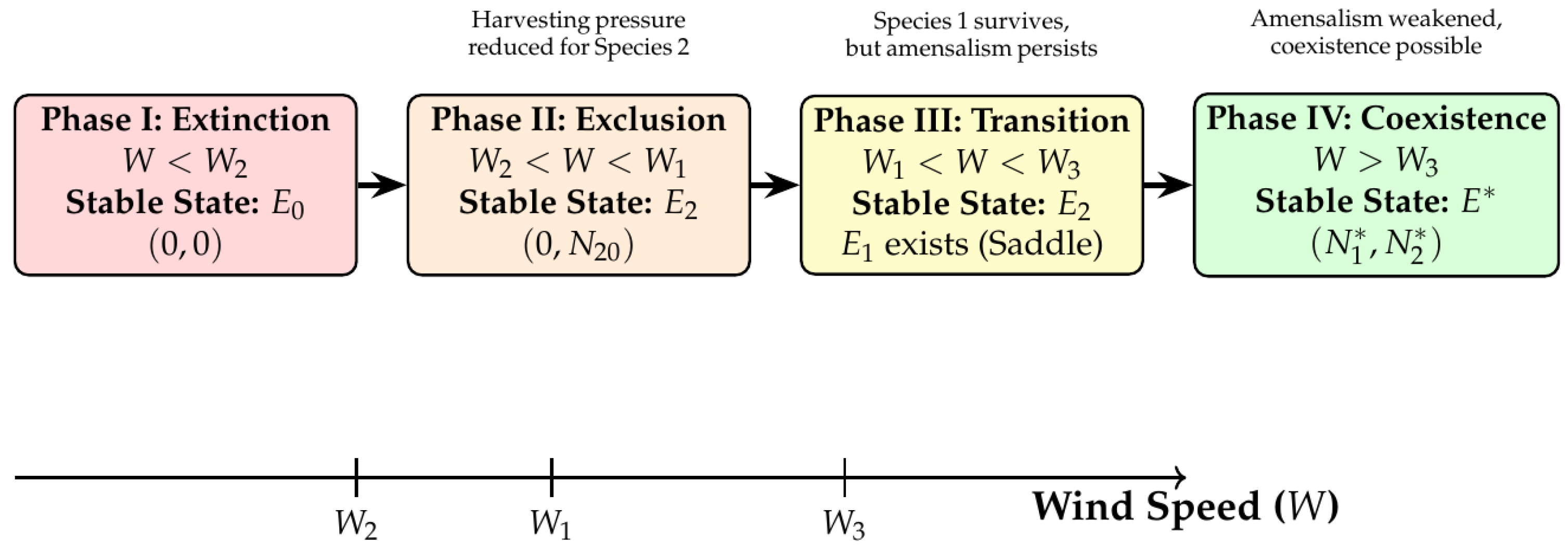
Figure 1. Schematic diagram of ecological regime shifts driven by increasing wind speed under the parameter scenario W 2 < W 1 . The system progresses through four distinct phases: from extinction of both species through an exclusive phase dominated by the less vulnerable species (species 2) and finally to stable coexistence when wind speed exceeds the critical value W 3 . The transitions are driven by the dual mechanism of wind reducing effective harvesting effort and weakening the amensalism intensity.
Eng 06 00367 g001
Figure 2. Phase portrait demonstrating global extinction under high harvesting pressure ( W = 0.2 ). Trajectories starting from four different initial conditions all converge to the trivial equilibrium E 0 = ( 0 , 0 ) . This visually confirms the global stability of the extinction state when wind speed is below the critical threshold W 2 , as the effective harvesting effort overwhelms the growth capacity of both species.
Eng 06 00367 g002
Figure 3. Time series corresponding to the phase portrait in Figure 1. The population densities of both species 1 (solid lines) and species 2 (dashed lines) decline monotonically to zero over time regardless of initial abundance. This simulates an ecological collapse scenario due to unregulated harvesting under calm wind conditions.
Eng 06 00367 g003
Figure 4. Phase portrait illustrating the exclusive dominance of species 2 at moderate wind speed ( W = 0.5 ). All trajectories, regardless of initial population densities, converge to the boundary equilibrium E 2 = ( 0 , N 20 0.065 ) . This demonstrates the global stability of E 2 in the wind speed interval W 2 < W < W 1 . The extinction of species 1 occurs because its intrinsic growth rate remains insufficient to overcome the combined pressure of harvesting and amensalism ( r 1 < q 1 E ^ m ), while species 2, being less vulnerable to harvesting ( q 2 < q 1 ), first escapes extinction as wind reduces the effective harvesting effort.
Eng 06 00367 g004
Figure 5. Time series dynamics for both species at W = 0.5 . Species 1 (solid lines): Populations from all initial conditions decline monotonically to zero, confirming its inevitable extinction due to excessive harvesting pressure. Species 2 (dashed lines): All populations converge to a positive equilibrium N 20 0.065 , establishing a stable population. The contrasting fates highlight the role of differential catchability ( q 1 > q 2 ): wind-induced reduction in harvesting effort is sufficient to allow the less vulnerable species (species 2) to survive but not enough to rescue the more vulnerable one (species 1) from extinction.
Eng 06 00367 g005
Figure 6. Phase portrait for the transitional regime at W = 0.8 . Despite the existence of three equilibrium points, all trajectories are globally attracted to E 2 = ( 0 , 0.196 ) , where species 2 exclusively dominates. The boundary equilibrium E 1 = ( 0.035 , 0 ) functions as an unstable saddle point (trajectories are repelled from it), while the trivial equilibrium E 0 is also unstable. This configuration confirms that although species 1 can now overcome harvesting pressure in isolation ( r 1 > q 1 E ^ m ), the persistent amensal effect from species 2 ( u ^ 0.403 ) creates an “invasion barrier”, preventing species 1 from establishing a viable population and ultimately leading to its exclusion.
Eng 06 00367 g006
Figure 7. Species 1 ( N 1 ): failed invasion and extinction. Initial attempts to grow are ultimately suppressed. The population fails to establish itself and is driven to zero, not by harvesting but by the biological interference from species 2.
Eng 06 00367 g007
Figure 8. Species 2 ( N 2 ): stable dominance. The population successfully resists invasion and stabilizes at a higher level ( N 20 0.196 ) than in Case 2, benefiting from reduced harvesting pressure and its unchallenged amensal effect.
Eng 06 00367 g008
Figure 9. Phase portrait demonstrating stable coexistence under high wind speed ( W = 3.0 ). All trajectories from diverse initial conditions converge to the positive equilibrium E * = ( N 1 * 0.486 , N 2 0.732 ) , confirming its global asymptotic stability. The system has successfully transitioned from the extinction and exclusion regimes to a biodiversity-rich state. This coexistence is facilitated by the dual regulatory effect of wind: significantly reduced harvesting effort ( E ^ 0.223 ) alleviates anthropogenic pressure, while substantially weakened amensalism ( u ^ 0.263 ) minimizes the biological inhibition on species 1. The result is an ecologically resilient state where both species persist at sustainable population levels.
Eng 06 00367 g009
Figure 10. Species 1 ( N 1 ): recovery and stabilization. The population recovers from various initial densities and stabilizes at N 1 0.486 . This demonstrates the species’ ability to thrive once freed from the dual constraints of intense harvesting and strong amensalism.
Eng 06 00367 g010
Figure 11. Species 2 ( N 2 ): persistence at high density. The population maintains a robust equilibrium at N 2 0.732 , benefiting from reduced harvesting pressure, while its capacity to inhibit species 1 is sufficiently weakened to permit coexistence.
Eng 06 00367 g011
Table 1. Description of variables and parameters used in the wind-driven amensalism-harvesting model.
SymbolDescriptionEcological/Biological MeaningUnits
State Variables
N 1 ( t ) , N 2 ( t ) Population densitiesDensity of species 1 (affected) and species 2 (inhibitor) at time t.biomass·area−1
tTimetime
Core Parameters
r 1 , r 2 Intrinsic growth ratesMaximum per capita growth rate under ideal conditions.time−1
P 1 , P 2 Environmental carrying capacitiesMaximum population size supported by the environment.biomass·area−1
u 0 Basic amensalism coefficientIntensity of inhibition exerted by species 2 on species 1 under windless conditions.dimensionless
q 1 , q 2 Catchability coefficientsEfficiency of harvesting gear for each species; reflects relative vulnerability.(effort·time)−1
Γ Maximum harvesting effortTheoretical maximum level of fishing activity in the absence of wind.effort
mProportion of harvestable populationManagement parameter; the fraction of the population open to harvesting ( 1 m is protected).dimensionless
WWind speedKey environmental driving variable.speed (e.g., m·s−1)
α Wind mixing effect coefficientQuantifies how effectively wind promotes diffusion and dilution of inhibitory substances.speed−1
β Wind resistance coefficientQuantifies the constraining effect of wind on fishing operations.speed−1
Derived Functions
u ˜ ( W ) Effective amensalism coefficientWind-diluted inhibition intensity: u 0 1 + α W .dimensionless
u ˜ ( W ) Effective harvesting effortWind-reduced fishing effort: Γ e β W .effort
Table 2. Summary of equilibrium point existence conditions.
Equilibrium PointExistence ConditionsEcological State
E 0 = ( 0 , 0 ) Always existsBoth species extinct
E 1 = ( N 10 , 0 ) r 1 > q 1 E ˜ m Species 2 extinct, species 1 survives
E 2 = ( 0 , N 20 ) r 2 > q 2 E ˜ m Species 1 extinct, species 2 survives
E = ( N 1 , N 2 ) r 2 > q 2 E ˜ m N 1 > 0 Both species coexist
Table 3. Summary of global stability conditions and their ecological implications.
Stable StateMathematical ConditionsEcological Interpretation
Extinction ( E 0 ) r 1 q 1 E ^ m and r 2 q 2 E ^ m Ecological collapse: Harvesting pressure is too severe for either species to survive. This represents a fisheries management failure.
Species 1 only ( E 1 ) r 1 > q 1 E ^ m and r 2 q 2 E ^ m Exclusion by dominance: Species 2 is driven to extinction by overharvesting. Species 1, being less vulnerable or faster growing, dominates the ecosystem.
Species 2 only ( E 2 ) r 2 > q 2 E ^ m and r 1 ( 1 u ^ N 20 P 1 ) q 1 E ^ m Exclusion by amensalism: Species 1 is suppressed by the combined effect of amensalism from species 2 and harvesting pressure. Species 2 prevails.
Coexistence ( E ) E existsResilient ecosystem: Wind speed is sufficient to weaken both harvesting and amensalism, allowing both species to persist. This is the biodiversity-positive outcome.
Table 4. Model parameter values and their biological justification.
ParameterValueEcological ExplanationBiological Rationale
r 1 , r 2 1.0Intrinsic growth ratesStandardized to 1.0 to focus on the relative effects of harvesting vulnerability and amensalism, assuming moderate and equal reproductive capacity for both species.
P 1 , P 2 1.0Environmental carrying capacitiesStandardized to 1.0 to simplify the analysis, representing a normalized environment where population densities are expressed as a proportion of their maximum.
u 0 0.5Basic amensalism coefficientRepresents a moderate inhibitory effect of species 2 on species 1, strong enough to influence dynamics but not so overwhelming as to preclude coexistence under favorable conditions.
q 1 1.8Catchability coefficient of species 1Chosen to be higher than q 2 to simulate a species that is more vulnerable to harvesting (e.g., due to larger size, slower movement, or attraction to gear).
q 2 1.5Catchability coefficient of species 2Chosen to be lower than q 1 to simulate a species that is less vulnerable to harvesting (e.g., due to smaller size, behavioral avoidance, or different habitat use).
E 0 1.0Maximum harvesting effortRepresents the baseline fishing effort under ideal (windless) conditions, standardized to 1.0.
m0.8Proportion of harvestable populationReflects a scenario of high fishing pressure with only
20% of the habitat protected, demonstrating the model’s behavior under significant anthropogenic stress.
α 0.3Wind mixing effect coefficientDetermines the rate at which wind dilutes inhibitory substances. A value of 0.3 indicates a moderately effective mixing process.
β 0.5Wind resistance coefficientDetermines the rate at which wind suppresses fishing effort. A value of 0.5 reflects a sensitive fishery where operations are significantly curtailed by increasing wind speed.
Disclaimer/Publisher’s Note: The statements, opinions and data contained in all publications are solely those of the individual author(s) and contributor(s) and not of MDPI and/or the editor(s). MDPI and/or the editor(s) disclaim responsibility for any injury to people or property resulting from any ideas, methods, instructions or products referred to in the content.