Article

A Machine Learning-Optimized Robot-Assisted Driving System for Efficient Flexible Forming of Composite Curved Components

by
Wenliang Wang
1,
Hexuan Shi
1,
Xianhe Cheng
1,
Rundong Ding
1,
Junwei Sun
1,
Yuan Li
1,
Xingjian Wang
1,
Shouzhi Hao
1,
Jing Yan
1 and
Qigang Han
1,2,3,*
1
Key Laboratory of Automobile Materials, Ministry of Education, School of Materials Science and Engineering, Jilin University, Changchun 130022, China
2
Institute of Structured and Architected Materials, Liaoning Academy of Materials, Shenyang 110167, China
3
Weihai Institute for Bionics, Jilin University, Weihai 264207, China
*
Author to whom correspondence should be addressed.
Eng 2025, 6(12), 356; https://doi.org/10.3390/eng6120356
Submission received: 2 November 2025 / Revised: 29 November 2025 / Accepted: 4 December 2025 / Published: 7 December 2025

Abstract

Flexible forming technology breaks through the traditional reliance on rigid molds in the hot-pressing process and demonstrates great potential for fabricating large, lightweight composite components with curved geometries. However, the precise actuation and error control of discrete units in flexible molds remain key technical challenges in the flexible forming of composites. This study proposes a high-precision and efficient method for the shape adjustment and error compensation of flexible multi-point molds. The proposed approach integrates the tangential offset unit configuration (TOUC) algorithm with an industrial robot to establish a robot-assisted precision driving system (RAPDS) for flexible molds. Furthermore, the main error-influencing factors of RAPDS are identified through correlation analysis and response surface modeling (RSM). Based on these findings, a backpropagation neural network (BPNN) is employed to predict adjustment errors, and heuristic algorithms guided by the structural characteristics of the BPNN are embedded into the framework to construct a bi-level optimization strategy that enhances model performance. The experimental results show that, compared with traditional methods, the robot-assisted flexible mold driving system improves the accuracy of shape adjustment by 31.0% and increases the production efficiency of composite components by 66.7%. Overall, this study develops a rapid, efficient, and highly precise flexible multi-point forming method for composite components, demonstrating strong potential for industrial applications.

1. Introduction

Fiber-reinforced composites (FRCs), owing to their outstanding mechanical properties and high design flexibility, have been extensively utilized in the aerospace [1], rail transit [2], and marine sectors [3]. With the continuous pursuit of lightweight and high-performance structures, the manufacturing of FRC components has been progressively shifting from small-scale integration toward large-scale, monolithic production [4]. However, traditional hot-press forming processes that depend on fixed molds lack flexibility [5], since each new component with a different curvature or geometry requires mold re-fabrication, which consequently leads to extended production cycles, increased manufacturing costs, and decreased efficiency [6]. Among these approaches, multi-point flexible forming technology can efficiently reconstruct mold surfaces by adjusting the height combinations of its discrete units [7], thereby enabling the generation of various geometric shapes [8]. Nevertheless, the height adjustment process of supporting units involves coordinated control among multiple systems and devices, often resulting in deviations between actual and preset heights. These errors cause discrepancies between the die surface and the target geometry [9,10], reducing geometric accuracy and forming quality. In severe cases, they may even lead to part rejection, consequently lowering both manufacturing efficiency and engineering applicability. Therefore, achieving precise actuation of mold surface supporting units has become a key challenge in improving forming quality and production efficiency in FRC flexible manufacturing.
To address actuation errors in supporting units of multi-point flexible forming technology, various numerical control methods have been developed, including motor arrays [11,12], hydraulic systems [13,14], and limit-sensor feedback mechanisms [15]. Although these methods can improve the level of automation and typically raise the initial adjustment accuracy to about 0.3–1 mm [16], they still suffer from high integration complexity and maintenance costs, and their residual positioning errors remain incompatible with the precision and stability requirements of flexible FRC manufacturing. In contrast, industrial robots exhibit significant advantages in complex surface machining and trajectory control. With superior spatial flexibility and high repeatability [17,18,19,20], they offer improved path accuracy and system integration [21,22,23], making them particularly suitable for three-dimensional surface adjustment in in multi-point flexible forming technology. However, the overall performance of such robotic-driven systems still depends on accurate modeling and reliable realization of theoretical adjustment heights. Hence, accurately determining the theoretical adjustment heights of FRC surfaces has become a crucial prerequisite for further enhancing adjustment precision.
Existing methods for determining theoretical adjustment heights typically rely on contact points between punches and the target surface. Researchers commonly employ computer-aided design (CAD) or computer-aided engineering (CAE) platforms for geometric modeling, where theoretical punch strokes are obtained through nonlinear inverse algorithms [24,25]. Although these methods provide certain geometric adaptability, they tend to produce large height errors in high-curvature regions and fail to maintain the surface continuity required for stable forming operations [26]. Moreover, traditional modeling workflows depend heavily on specialized platforms, leading to high computational costs and limited interactivity. These constraints restrict adaptability to various geometries and hinder efficient transitions between manufacturing tasks. To overcome these limitations, this study proposes a tangential offset Unit configuration (TOUC) algorithm implemented via the Rhino8-Python interface. This method supports parametric control and visual interaction, enabling the automatic generation of complex punch arrays and the extraction of their theoretical heights. The proposed approach improves modeling efficiency, reduces computational load, enhances flexibility, and significantly broadens modeling applicability. Nevertheless, even with optimized modeling and actuation systems, non-ideal factors such as equipment errors and load disturbances can still cause deviations between the adjusted surface and the target geometry.
During the actuation process of supporting units in multi-point flexible forming technology, compensating for height deviations is essential to ensure the dimensional accuracy of three-dimensional surfaces. Conventional methods typically rely on post-adjustment measurements to identify error distributions and iteratively modify support unit heights to gradually approximate the target geometry [16]. Although this iterative process can improve accuracy, the discrete punch structure of multi-point flexible forming technology often leads to error coupling [27], which reduces both surface reconstruction efficiency and system stability. Moreover, heavy dependence on measurement and control processes limits compensation speed and responsiveness, particularly for complex surfaces [28,29,30]. To overcome these challenges, researchers have explored compensation strategies based on error prediction [31,32,33]. Among these approaches, the backpropagation neural network (BPNN) has garnered considerable attention due to its strong nonlinear mapping capability and excellent generalization performance under small-sample conditions [34,35], enabling it to effectively model the relationship between adjustment parameters and errors [36]. However, BPNNs are prone to local optima, exhibit slow convergence, and are sensitive to initial weights [37], restricting their applicability in high-precision adjustments. To enhance performance, metaheuristic optimization algorithms have been introduced to jointly optimize network architectures and parameters, thereby improving convergence speed, accuracy, and robustness [38,39]. Nevertheless, studies focusing on applying BPNNs to predict and compensate for actuation errors in multi-point flexible forming technology remain limited. Consequently, implementing a bi-level structural optimization strategy that integrates metaheuristic algorithms is expected to effectively improve prediction and compensation accuracy for supporting units in multi-point flexible forming technology.
To address the problems of low actuation accuracy and poor error control of the discrete units in multi-point flexible forming molds, this study develops a robot-assisted precision driving system for the flexible manufacturing of FRC components. In terms of the precise actuation of discrete units, a tangential offset unit configuration (TOUC) algorithm is developed in Rhino-Python to enable efficient alignment of the punch head with complex curved surfaces and to automatically generate the theoretical adjustment heights. For error prediction and compensation of supporting unit actuation in multi-point flexible forming technology, correlation analysis and response surface methodology (RSM) are employed to identify the primary factors causing errors during the supporting unit height actuation process of the robot-assisted precision driving system. Based on these findings, a backpropagation neural network (BPNN) framework with a bi-level optimization strategy is constructed to predict the adjustment errors of supporting units. The predicted errors are directly applied to the theoretical heights to form a feedforward error-compensation mechanism. Finally, a fiber-reinforced composite (FRC) flexible manufacturing method integrating actuation optimization and error compensation is established, which significantly improves the forming accuracy and manufacturing efficiency of components.

2. Robot-Assisted Precision Driving System

In this section, a robot-assisted precision driving system (RAPDS) for multi-point flexible forming molds is introduced. This system integrates the self-developed tangential offset unit configuration (TOUC) algorithm with an industrial manipulator to reconstruct the forming surface according to the target fiber-reinforced composite (FRC) geometry. The system is also equipped with a non-contact laser measurement unit that enables precise error detection, ensuring consistency between the forming surface and the desired FRC contour.

2.1. Flexible Mold Shape Regulation System

The tangential offset unit configuration (TOUC) algorithm is illustrated in Figure 1. First, the geometric surface of the fiber-reinforced composite (FRC) component is translated pointwise along its unit normal vectors by a distance equal to the radius of the spherical punch tip (d = 16 mm; Figure 1a) to generate the offset surface S o f f s e t . This auxiliary surface ensures tangential conformity with the original geometry. Subsequently, a spherical fitting algorithm is applied to the punch tip to determine the punch-center coordinates C p u n c h = x c , y c , z c (Figure 1b). The punch center is then vertically projected onto the offset surface, yielding the projection point P p r o j = x p , y p , z p (Figure 1c). The vertical displacement is defined as:
Δ Z = z c z p
This displacement serves as the adjustment reference for calibrating the height of each punch unit. By applying this correction, the punch array can be theoretically aligned with the target FRC surface (Figure 1d).
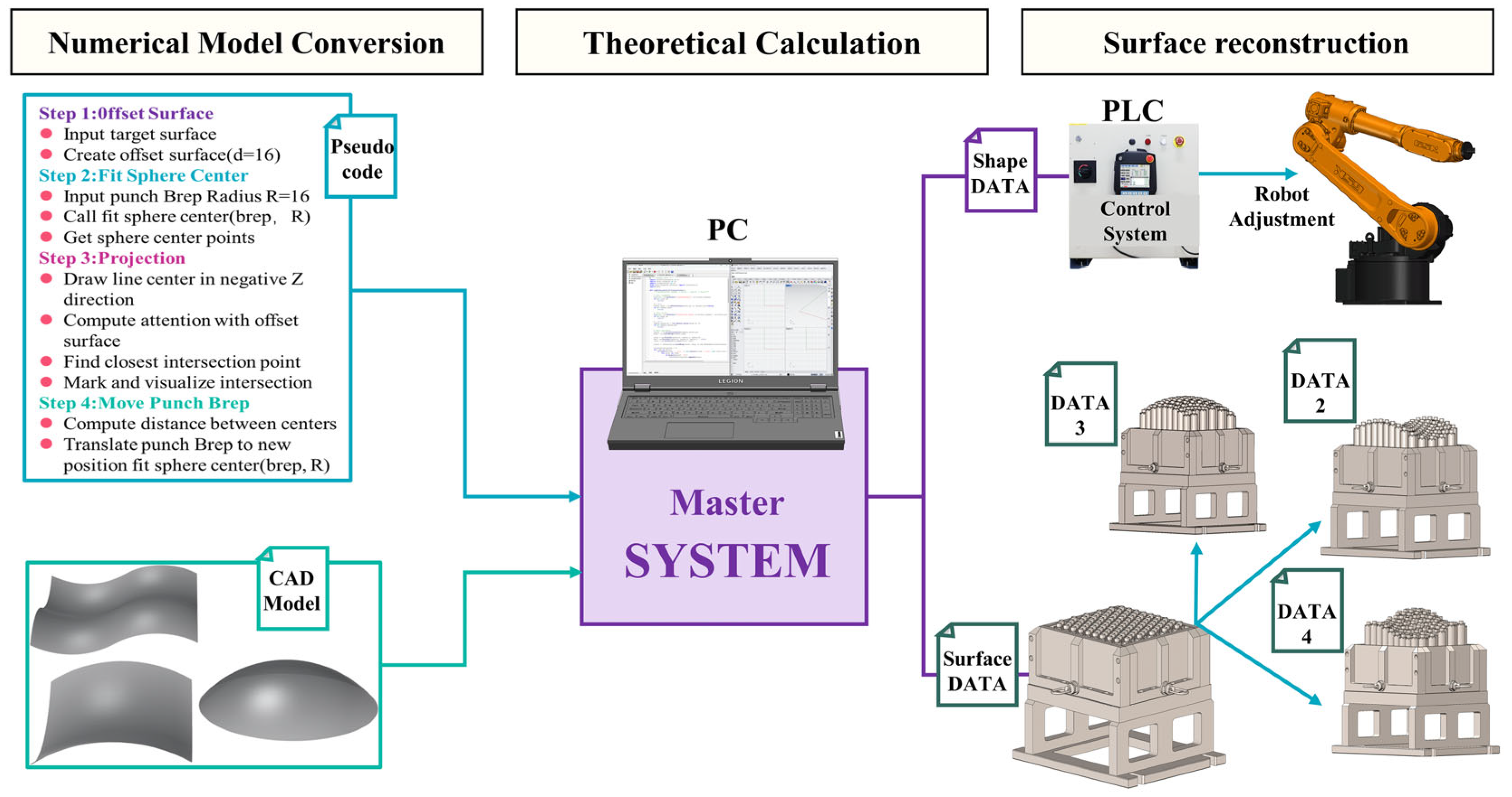
As shown in Figure 2, the robot-assisted precision driving system (RAPDS) incorporates the TOUC algorithm within a three-stage workflow consisting of numerical model conversion, theoretical computation, and surface reconstruction. In the numerical model conversion stage, the CAD surface is processed in Rhino using the TOUC algorithm to obtain the target punch-height distribution. During the theoretical computation stage, the master computer (PC) compiles the geometric results into a punch-height adjustment table that specifies the required ΔZ for each punch unit. In the surface reconstruction stage, these computed values are transmitted through a programmable logic controller (PLC) to an industrial robot (RB20A3; repeatability ±0.02 mm), which sequentially calibrates the punch array.
To facilitate efficient switching between different forming tasks, the RAPDS allows the use of multiple predefined data configurations. DATA 2, DATA 3, and DATA 4 correspond to three representative punch-height datasets, each derived from a distinct typical FRC target surface. These datasets serve as input configurations for driving the robot to rapidly reconfigure the multi-point flexible forming mold, enabling the system to adapt to different curved surface geometries without re-running the full modeling workflow.

2.2. Flexible Mold Shape Errors Measurement System

A non-contact laser measurement system was developed to enable precise error quantification and support data-driven modeling during multi-point flexible forming mold adjustments, as illustrated in Figure 3. The system integrates a BLG laser displacement sensor (with a measurement accuracy of 0.01 mm) mounted on the end effector of an industrial manipulator (RB20A3, Brand BIJKE, made in Guangdong, China). This configuration allows the robot to sequentially scan each punch unit along a predefined path, acquiring both the initial punch height h 0 and the post-adjustment height h 1 . The actual height increment for each punch was calculated as:
h = h 0 h 1
The adjustment error was then determined by comparing the measured increment Δ h a c t u a l with the theoretical increment Δ h t h e o r e t i c a l specified in the experimental design:
y = h t h e o r e t i c a l Δ h a c t u a l
By integrating non-contact laser sensing with robot-driven adaptive measurement paths, the system significantly improves the efficiency and accuracy of adjustment error acquisition.

3. Analysis of RAPDS Errors

In this section, six factors closely related to the actuation process of support unit heights in the robot-assisted precision driving system (RAPDS) were systematically analyzed. A dataset of 200 randomly sampled adjustment-error measurements was collected to evaluate the correlations between these errors and the six factors. In addition, a Box–Behnken design comprising 54 experimental runs was constructed in Design-Expert to assess factor significance and quantify each factor’s effect on adjustment error.

3.1. Correlation Factors Analysis

For this analysis, 200 adjustment error samples were collected from RAPDS to investigate the factors contributing to adjustment deviations. Six candidate input variables were selected based on their physical relevance to the actuation of the robot’s end effector and the structural characteristics of the multi-point flexible forming mold, as these components represent primary sources of error in the adjustment process. These variables include theoretical forming height (X1), radial distance from the mold center (X2), adjustment sequence (X3), ambient temperature (X4), initial surface deviation (X5), and motor speed level (X6). The adjustment error (Y), defined as the signed deviation between the target punch height and the robot-adjusted punch position, was treated as the response variable in this analysis.
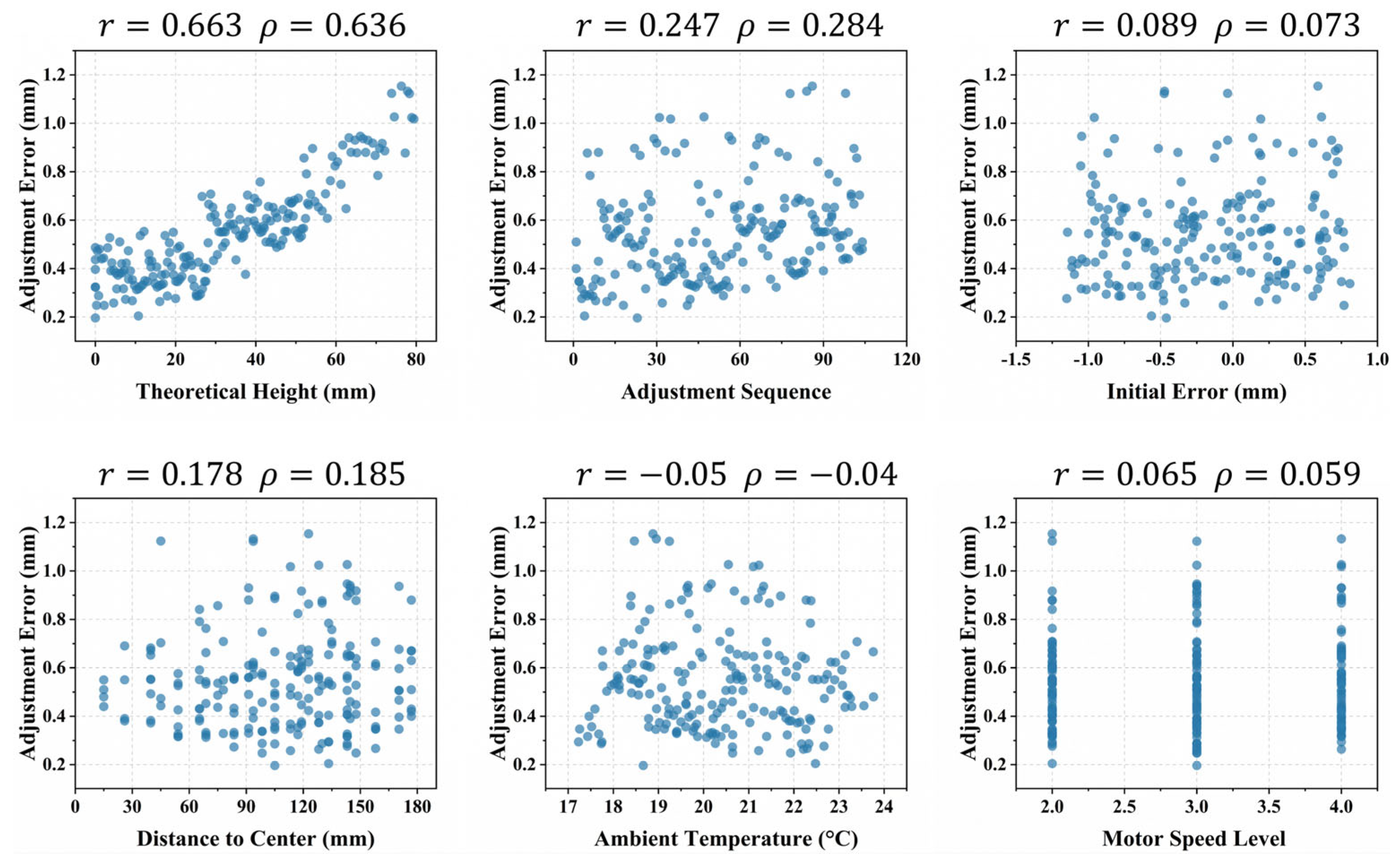
As illustrated in Figure 4, the relationships between Y and the six input variables were evaluated using Pearson’s correlation coefficient (PCC, r ) to quantify linear associations and Spearman’s rank correlation coefficient (SRC, ρ ) to assess monotonic trends. X1 exhibited the strongest positive correlation with Y ( r = 0.663, ρ = 0.636). This relationship indicates that larger theoretical adjustment heights tend to yield higher adjustment deviations. This trend is attributed to the increased kinematic travel required by the robot, where larger displacements amplify the accumulation of positioning errors and mechanical actuation inaccuracies in the end-effector. X3 showed a moderate correlation ( r = 0.247, ρ = 0.284), indicating that sequential adjustments can propagate cumulative errors across the system. In contrast, X2 ( r = 0.178, ρ = 0.185) displayed a weak positive correlation; this may be attributed to the discrete structural characteristics of the multi-point flexible forming mold, where reduced stiffness at the mold edges increases susceptibility to deformation. The remaining variables, including ambient temperature X4 ( r = −0.05, ρ = −0.04), initial surface deviation X5 ( r = 0.089, ρ = 0.073), and motor speed level X6 ( r = 0.065, ρ = 0.059), exhibited negligible correlations with Y (∣ r ∣, ∣ ρ ∣ < 0.2), suggesting minimal direct effects on adjustment errors under the tested conditions.

3.2. Significant Factors Analysis

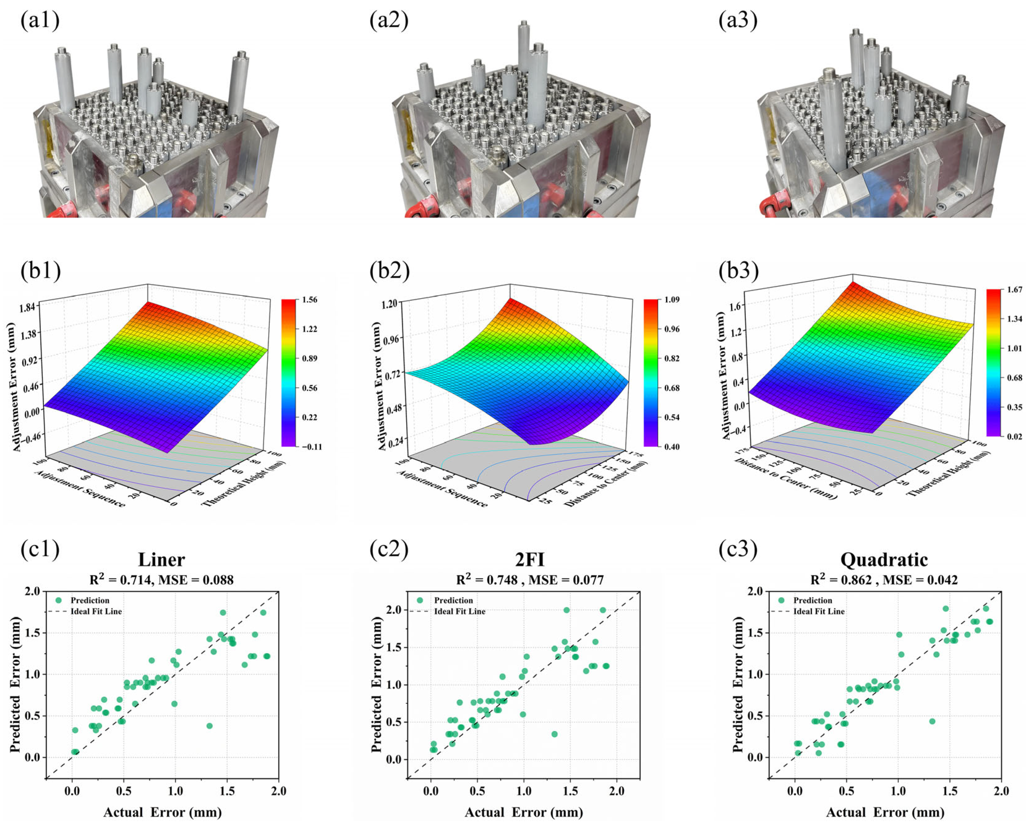
Response surface methodology (RSM) [40], based on the Box–Behnken design, was employed to investigate the influence of six candidate factors: theoretical height (X1), radial distance from the mold center (X2), adjustment sequence (X3), ambient temperature (X4), initial surface deviation (X5), and motor speed level (X6), on adjustment error (Y). This framework enabled a systematic evaluation of factor interactions and their combined effects on multi-point flexible forming mold adjustment accuracy. The experimental matrix included 54 parameter combinations (Table 1), implemented using the RAPDS described in Section 2. As shown in Figure 5(a1–a3), each run controlled all six variables, with the resulting adjustment error recorded as the response variable.
Building upon the correlation analysis in Section 3.1, a combined evaluation was conducted using Pearson’s correlation coefficient (r), Spearman’s rank correlation coefficient (ρ), and analysis of variance (ANOVA) to comprehensively assess factor significance. As summarized in Table 2, theoretical height (X1), radial distance (X2), and adjustment sequence (X3) were consistently identified as significant predictors of adjustment error (p < 0.05). In particular, X1 exhibited the strongest effect (r = 0.663, ρ = 0.636; F = 63.72, p = 0.001), indicating that larger theoretical heights may amplify positioning and actuation deviations due to cumulative effects during robotic adjustments. X3 showed a moderate effect (r = 0.247, ρ = 0.284; F = 34.96, p = 0.001), likely resulting from sequential error accumulation and thermally induced precision degradation of the end-effector during extended operation. X2 exhibited marginal significance (r = 0.178, ρ = 0.185; F = 4.21, p = 0.05), potentially due to structural discreteness and reduced stiffness near mold edges. In contrast, X4, X5, and X6 were statistically insignificant (p > 0.05).
Based on these findings, regression models incorporating X1, X2, and X3 were developed to analyze nonlinear relationships and interaction effects. The fitted response surfaces in Figure 5(b1–b3) revealed distinct nonlinear interactions among these variables. Model performance evaluation Figure 5(c1–c3) demonstrated that the quadratic model achieved the highest predictive accuracy (R2 = 0.862, MSE = 0.042), outperforming the linear (R2 = 0.714, MSE = 0.088) and 2FI (R2 = 0.748, MSE = 0.077) models. These results emphasize the necessity of incorporating nonlinear and interaction terms when modeling adjustment errors in the RAPDS.

4. Bi-Level Optimized BPNN Error Prediction Modeling

4.1. BPNN Model

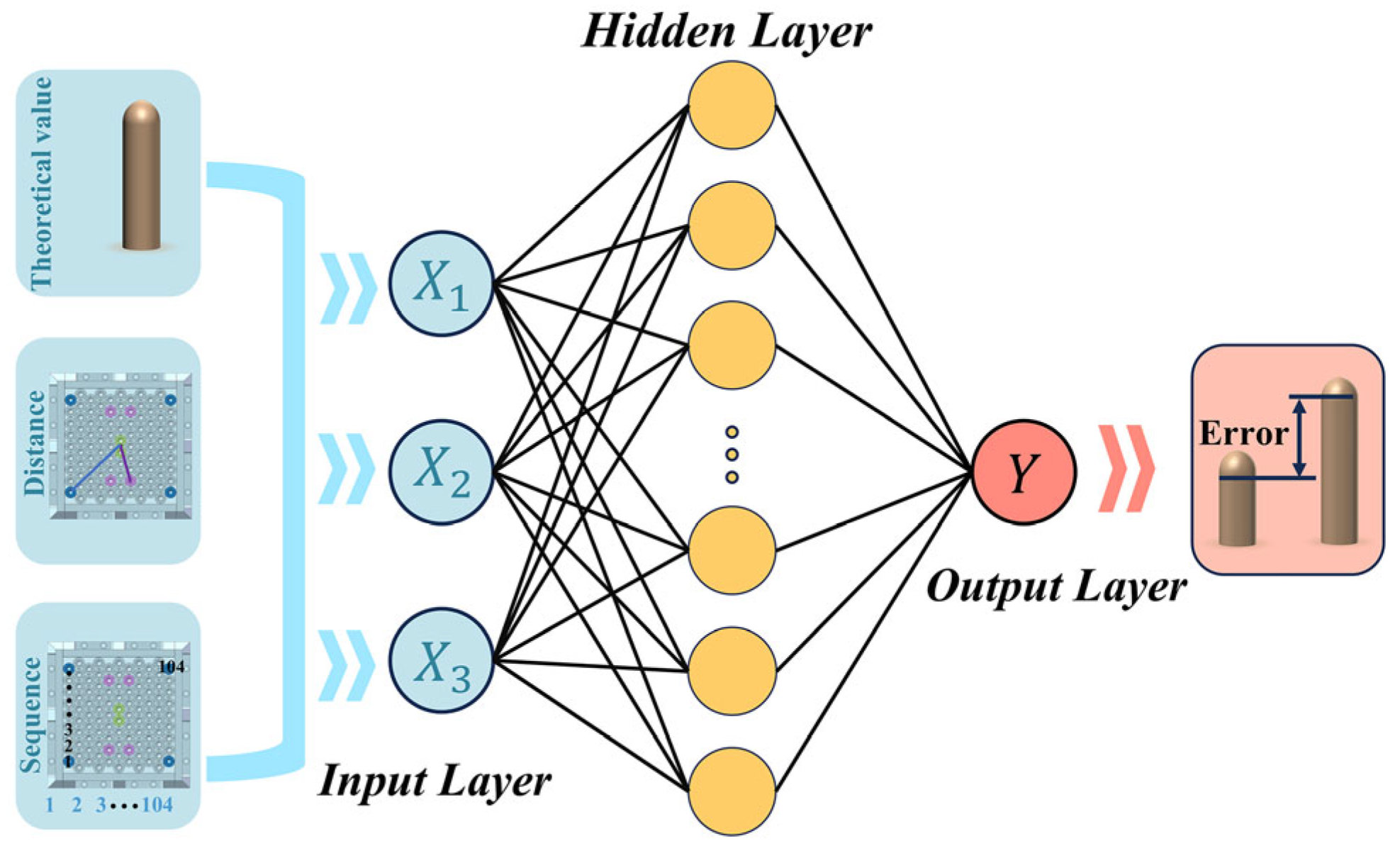
In view of the nonlinear dependencies identified in Section 3.2, a baseline backpropagation neural network (BPNN) was developed to model the complex relationships between key influencing factors and adjustment errors in the robotic height adjustment system (RHAS). As illustrated in Figure 6, the network architecture consists of an input layer with three nodes corresponding to the significant variables: theoretical height (X1), radial distance from the die center (X2), and adjustment sequence (X3); a hidden layer for feature extraction and nonlinear mapping; and an output layer with a single node representing the predicted adjustment error (Y).
To enhance the network’s ability to capture complex nonlinear patterns, the hidden layer employs the hyperbolic tangent sigmoid activation function (tansig):
( x ) = 2 1 + e 2 x 1
This function facilitates smooth transitions and constrains the outputs within (−1, 1), which improves convergence during backpropagation. The output layer uses a linear activation function (purelin), defined as:
f ( x ) = x
allowing continuous predictions suitable for regression tasks. The BPNN was trained using the standard backpropagation algorithm to minimize the mean squared error (MSE) between predicted and actual adjustment errors, calculated as:
M S E = 1 n i = 1 n   ( y i y ^ i ) 2
where y i and y ^ i represent the actual and predicted adjustment errors for the ith sample, respectively, and n denotes the total number of samples.

4.2. Bi-Level Optimization Strategy

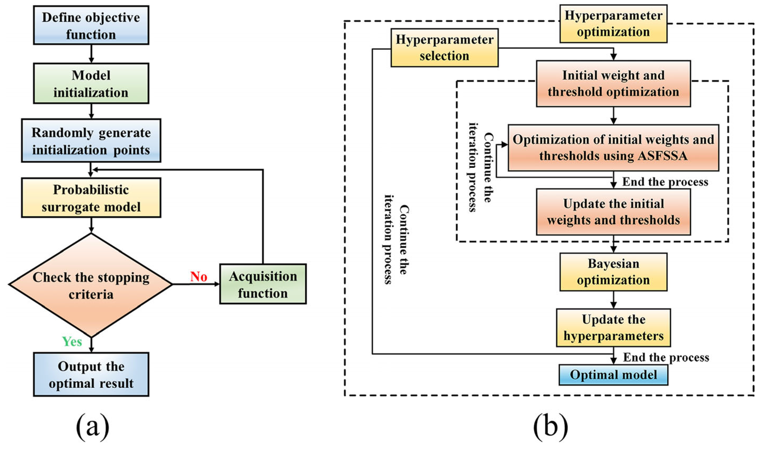
To address the challenges of parameter sensitivity and convergence instability commonly encountered in neural networks, this study proposes a bi-level optimization strategy that integrates Bayesian Optimization (BO) and the Adaptive Spiral Flight Sparrow Search Algorithm (ASFSSA) [41], as depicted in Figure 7b. This approach is designed to systematically tune critical hyperparameters and refine the initial weights and biases of the network. The underlying objective is to improve the predictive performance and robustness of the error compensation model by enhancing convergence stability and reducing entrapment in local minima.

4.2.1. BO-Based Hyperparameter Optimization

BO was applied to efficiently search the hyperparameter space of the BPNN and identify configurations that minimize the root mean square error (RMSE) on the training dataset:
f η , H = R M S E η , H
as illustrated in Figure 7a, BO uses Gaussian Process Regression (GPR) to build a surrogate model of the objective function f . For each candidate configuration x, the predictive mean μ ( x ) and variance σ 2 ( x ) are computed as:
μ ( x ) = k ( x , X ) K ( X , X ) + σ n 2 I 1 y
σ 2 ( x ) = k ( x , x ) k ( x , X ) K ( X , X ) + σ n 2 I 1 k ( X , x )
where k ( , ) denotes the kernel function, K ( X , X ) is the covariance matrix of observed data X and σ n 2 represents the noise variance. The Expected Improvement (EI) acquisition function guides the search process:
E I x = E m a x f b e s t f x , 0
this process iterates until convergence or a maximum of 20 iterations, yielding optimal hyperparameters ( η * , H * ) for BPNN training.

4.2.2. ASFSSA-Based Weight and Bias Initialization

ASFSSA was applied to globally optimize the initial weights and biases of the BPNN, addressing convergence instability caused by random parameter initialization. ASFSSA enhances the standard Sparrow Search Algorithm (SSA) by introducing adaptive spiral flight patterns to balance global exploration and local exploitation during the search process.
In this framework, all trainable parameters of the BPNN, namely the weights from the input layer to the hidden layer, the weights from the hidden layer to the output layer, and the biases of both layers, are encoded into a high dimensional decision vector. The dimensionality of this vector is defined as:
D = I × H + H × O + H + O
where I, H, and O represent the numbers of neurons in the hidden input, and output layers, respectively.
To enhance population diversity and improve exploration, a Tent chaotic map is used to initialize the population:
z i + 1 = 2 z i + r a n d ( 0,1 ) 1 N , 0 z 1 2 2 ( 1 z i ) + r a n d ( 0,1 ) 1 N , 1 2 z 1
The resulting chaotic values z i , j are scaled into the actual search space using:
x i , j = l b j + u b j l b j z i , j
where x i , j is the jth dimension of the ith individual, and l b j , u b j denote the lower and upper bounds for the jth parameter.
The fitness function is defined as the root mean square error (RMSE) on the training dataset:
R M S E = 1 n i = 1 n   ( y i y ^ i ) 2
where y i and y ^ i denote the actual and predicted outputs for the ith sample, respectively, and n is the total number of samples.
During the discoverer phase, ASFSSA integrates a time-adaptive spiral flight mechanism to update individual positions:
x i t + 1 = w ( t ) x i t e x p r 1 i t
where the adaptive weight function w ( t ) is given by:
w t = 0.2 cos π 2 1 t t m a x
here, r 1 0 ,   1 is a uniformly distributed random number, t is the current iteration, and t m a x is the maximum number of iterations. To improve the algorithm’s ability to escape local optima, a Levy flight mechanism is incorporated:
L e v y ( β ) = μ | ν | 1 / β , μ N ( 0 , σ 2 ) , ν N ( 0,1 )
During the joiner phase, individuals perturb the current global best solution using:
x i t + 1 = x b e s t + ϵ r a n d n 1 , D x i t x b e s t
where ϵ is a scaling parameter and r a n d n 1 , D denotes a D-dimensional Gaussian random vector. The optimization process terminates when a predefined precision criterion is met or the maximum number of iterations is reached. The best individual found yields the optimal weight vector W * and bias vector b * for initializing the BPNN, thereby improving convergence stability and prediction accuracy.

4.3. Data Validation

The proposed BO-ASFSSA-BPNN model was trained and validated through simulation in MATLAB 2022b, utilizing 2080 adjustment error samples collected from the experimental platform (Section 2.2) after removing outliers and anomalous data points to ensure data reliability. Based on the hyperparameter optimization results from Section 4.2.1, the optimal configuration ( H * , η * ) was determined by minimizing the root mean square error (RMSE) on the training dataset:
m i n H , η   R M S E t r a i n ( H , η )
Subsequently, the initial weights (W) and biases (b) were optimized globally using ASFSSA (Section 4.2.2) to refine network initialization and improve convergence:
m i n W , b   R M S E t r a i n ( W , b | H * , η * )
After outlier removal, the dataset was randomly partitioned into a training set (80.0%) and a testing set (20.0%), and all input variables were normalized to [0, 1] to enhance convergence speed. The training was conducted with a maximum of 100,000 iterations and an error threshold of 10−7, ensuring high-precision learning in the MATLAB simulation environment.
To evaluate the predictive performance of the BO-ASFSSA-BPNN model, four widely used regression metrics were employed: coefficient of determination (R2), root mean square error (RMSE) (14), mean absolute error (MAE), and mean absolute percentage error (MAPE):
R 2 = 1 ( y i y ^ i ) 2 ( y i y ¯ ) 2
M A E = 1 n y i y ^ i
M A P E = 100.00 % n i = 1 n   y ^ i y i y i
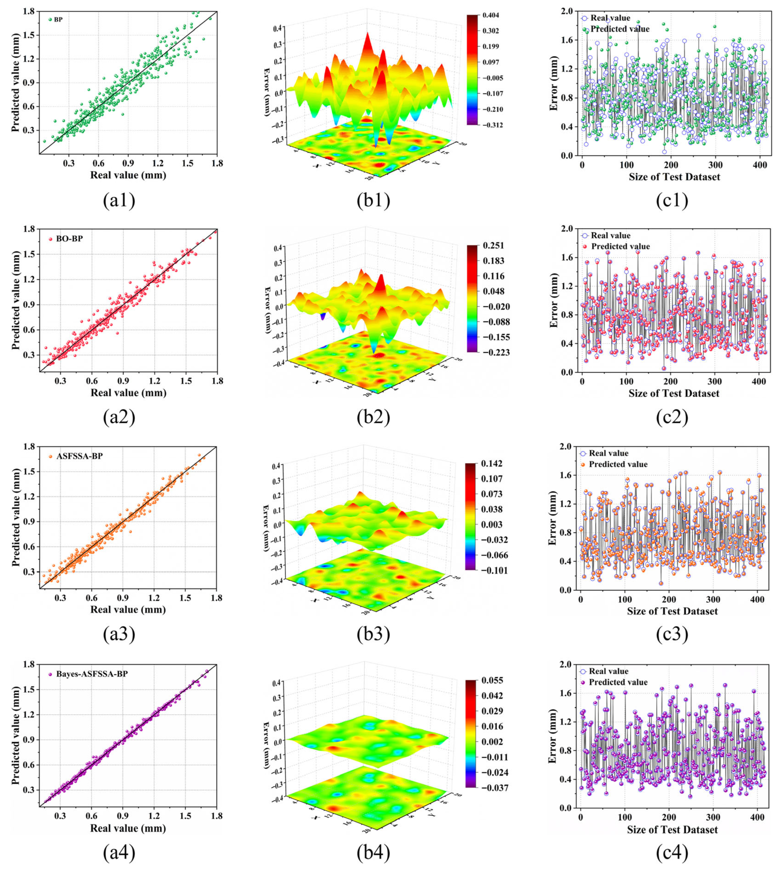
To evaluate the predictive performance of different models, BPNN, BO-BPNN, ASFSSA-BPNN, and BO-ASFSSA-BPNN were comparatively analyzed using statistical measures including R2, RMSE, MAE, MAPE, and training time (Table 3). The baseline BPNN exhibited limited accuracy (R2 = 0.9089, RMSE = 0.1112) but required the least computational time (2.00 s). The introduction of Bayesian Optimization (BO-BPNN) significantly improved performance, reducing RMSE and MAPE by more than 50.0% compared with the baseline, with a moderate increase in training time to 4.19 s. Further refinement through ASFSSA optimization (ASFSSA-BPNN) yielded lower prediction errors but incurred the highest computational cost (20.00 s). The combined BO-ASFSSA-BPNN model achieved the best results, with R2 = 0.9973, RMSE = 0.0218, MAE = 0.0148, and MAPE = 2.2%. Moreover, this hybrid model demonstrated improved efficiency compared to ASFSSA-BPNN by reducing the training time to 16.14 s, indicating a substantial improvement in accuracy and generalization without maximizing computational burden.
The visual comparisons in Figure 8 reinforce these findings. As shown in Figure 8(a1–a4), the predicted values of each successive model become progressively closer to the actual values, consistent with the observed rise in R2. The residual surfaces Figure 8(b1–b4) further demonstrate this trend: the error distribution evolves from a wide and uneven range in BPNN to a nearly flat surface centered around zero in BO-ASFSSA-BPNN, thereby confirming improved convergence and reduced bias. Finally, the error trends across the test dataset Figure 8(c1–c4) reveal that the dual-optimized model exhibits the smallest fluctuations and the most stable tracking of real values, verifying its superior predictive capability.

5. Compensation for RAPDS Adjustment Errors

To validate the engineering practicality of the proposed BO-ASFSSA-BPNN model, this section applies the trained model to predict height-adjustment errors of the RAPDS actuated support units and applied a feedforward error-compensation strategy to correct those errors. To evaluate the model’s potential in flexible forming scenarios, three representative 3D component surfaces were selected to assess its adjustment accuracy and stability.

5.1. Compensation Theory

To achieve effective error correction in the support unit height adjustment during the first adjustment of RAPDS, an error compensation strategy is proposed. This strategy aims to minimize the deviation of the target surface by incorporating multiple sources of error into the initial adjustment stage. After all support units are calibrated to the reference plane, the flatness deviation caused by inherent actuation errors or structural discrepancies is measured and denoted as the initial surface error ( δ i n i t ). This value is then embedded into the theoretical punch height to preemptively compensate for platform-induced errors. Meanwhile, the BO-ASFSSA-BPNN model is employed to predict surface errors arising from the complex geometry of target components, yielding the predicted adjustment error ( δ p r e d ). These two error components are then integrated with the ideal theoretical height ( Δ Z ) to obtain the compensated punch height ( H a d j ), which is defined as follows:
H a d j = Δ Z + δ i n i t + δ p r e d
This compensation strategy incorporates both the initial errors of the support units in the flexible multi-point mold and the errors of the RAPDS into the first adjustment stage. Consequently, it minimizes height deviations during the initial process, thereby improving the overall accuracy and robustness of the RAPDS.

5.2. Compensation Experiment

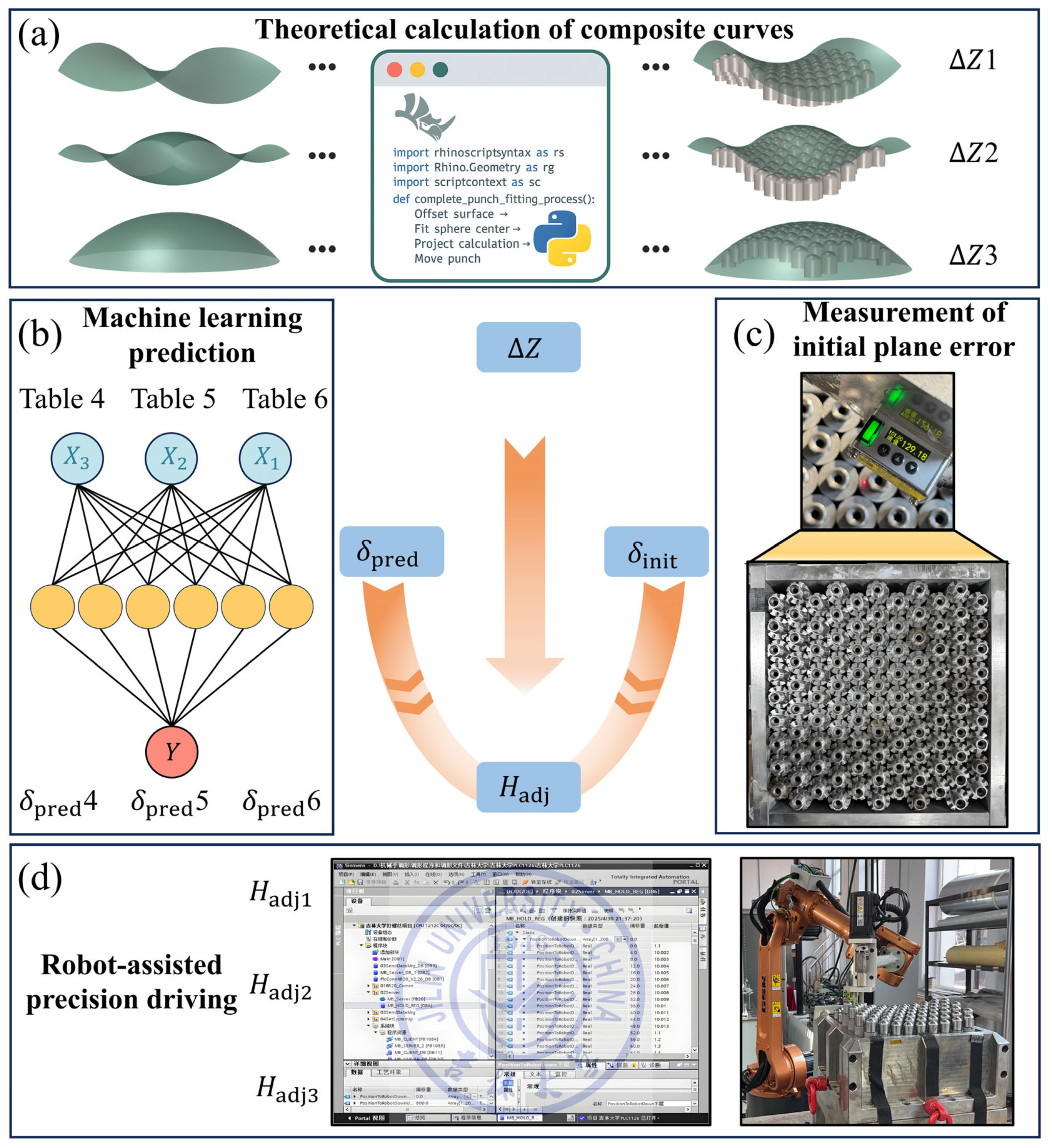
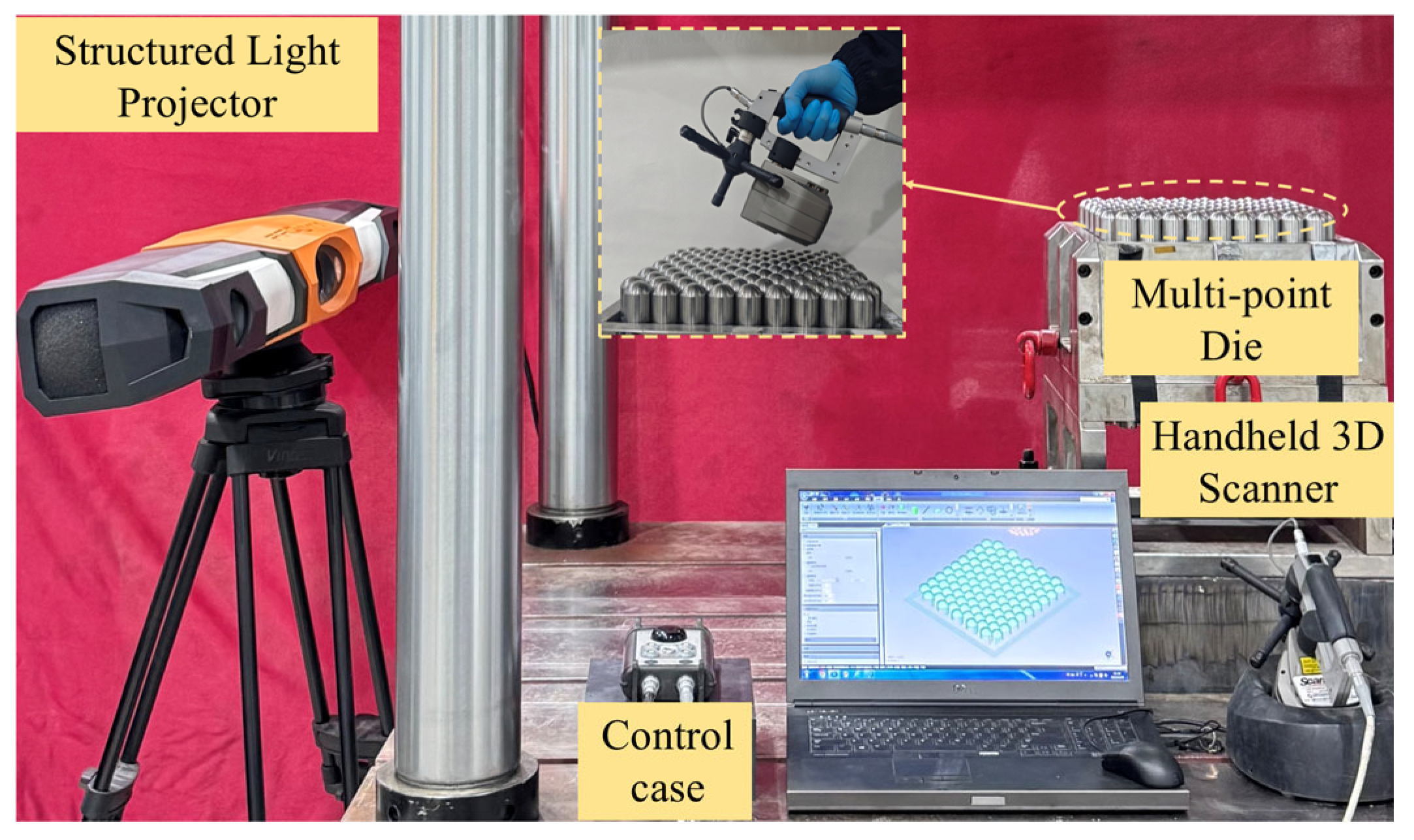
The CAD model of the target composite component is imported into Rhino, where the custom TOUC algorithm is applied to fit the multi-point punch units to the desired geometry. This process generates the theoretical forming surface and calculating the theoretical adjustment height for each punch Figure 9a. These theoretical heights are then input into the pre-trained BO-ASFSSA-BPNN model to efficiently and accurately predict the adjustment errors of the supporting units, Figure 9b. After aligning the punches with the reference plane, a laser displacement sensor is used to measure the initial planar deviation, Figure 9c. The theoretical heights, model-predicted errors, and measured deviations are then integrated into a unified adjustment command, which is uploaded to the robot controller to drive the supporting units of the flexible multi-point mold for height calibration. This process enables the combined heights of the supporting units to align the forming surface with the target geometry, Figure 9d. After the adjustment, the compensated surface formed by the supporting units is captured using a structured-light projector and a handheld 3D scanner, Figure 10, to obtain a high-density point cloud. The acquired point cloud data are then used to quantify the deviations between the compensated and theoretical heights, completing the closed loop for performance evaluation and further refinement.

6. Discussions

6.1. Error Adjustment on Baseline Shape

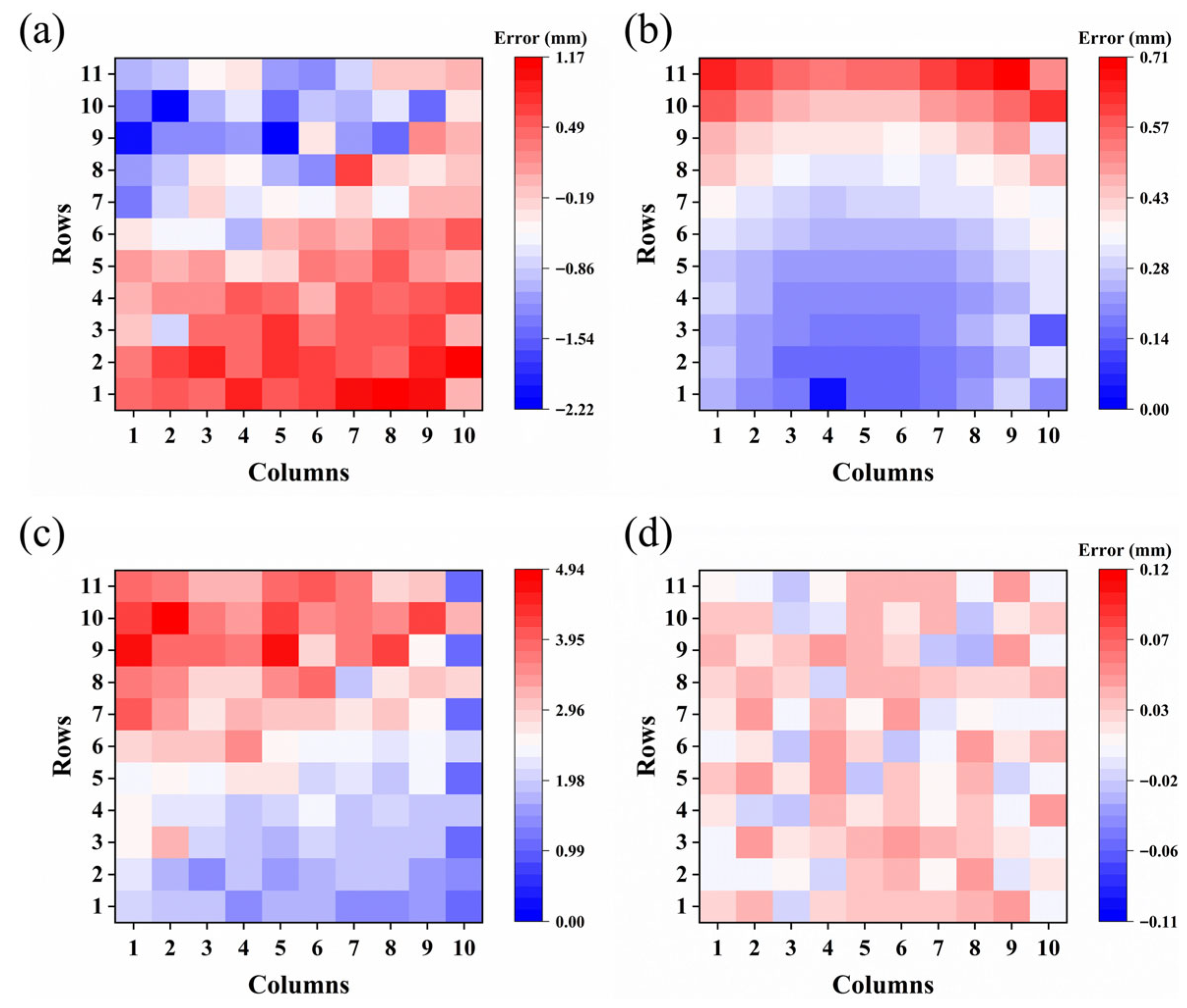
During the adjustment of complex composite component surfaces, the initial plane is aligned with the reference plane to minimize its impact on subsequent adjustment accuracy. Figure 11a shows the distribution of the initial surface error, with a maximum deviation of ±2.22 mm and significant regional differences. Subsequently, the trained BO-ASFSSA-BPNN model was applied to predict the adjustment error of each punch unit. As shown in Figure 11b, the predicted errors range from 0 to 0.71 mm, with a relatively concentrated distribution. The compensation values were then calculated based on the initial error, the predicted error, and the theoretical heights of the support units, as illustrated in Figure 11c. The robot then adjusted the support unit heights according to the calculated compensation values, and a laser displacement sensor was employed to measure the surface error of the flexible multi-point mold after adjustment. As shown in Figure 11d, the final surface error was controlled within ±0.12 mm, with an average error of approximately 0.04 mm, thereby verifying the effectiveness of the proposed compensation strategy in plane adjustment.

6.2. Evaluation of Method Effectiveness on Complex Shape

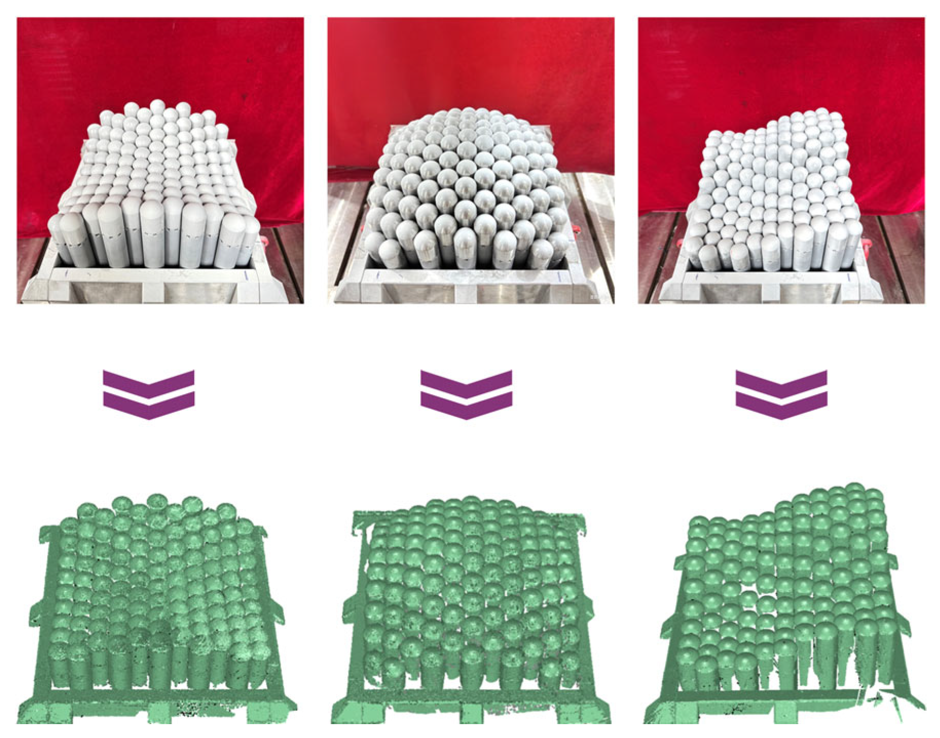
To further evaluate the applicability of the proposed compensation strategy for adjusting the support units of the flexible multi-point mold in RAPDS, high-precision 3D scanning was performed using a structured-light projector and a handheld 3D scanner Figure 10. This setup enabled the acquisition of dense point cloud data representing the adjusted surfaces of the flexible multi-point mold Figure 12. The acquired data were then processed in Geomagic Control X for denoising and dimensional analysis. Based on the filtered, high-quality point clouds, both a global 3D surface-deviation evaluation and a local 2D cross-sectional height-profile analysis were conducted. These analyses provided a quantitative assessment of the overall 3D surface adjustment accuracy and localized height deviations of the flexible multi-point mold support units, thereby verifying the adjustment performance across various complex component geometries.
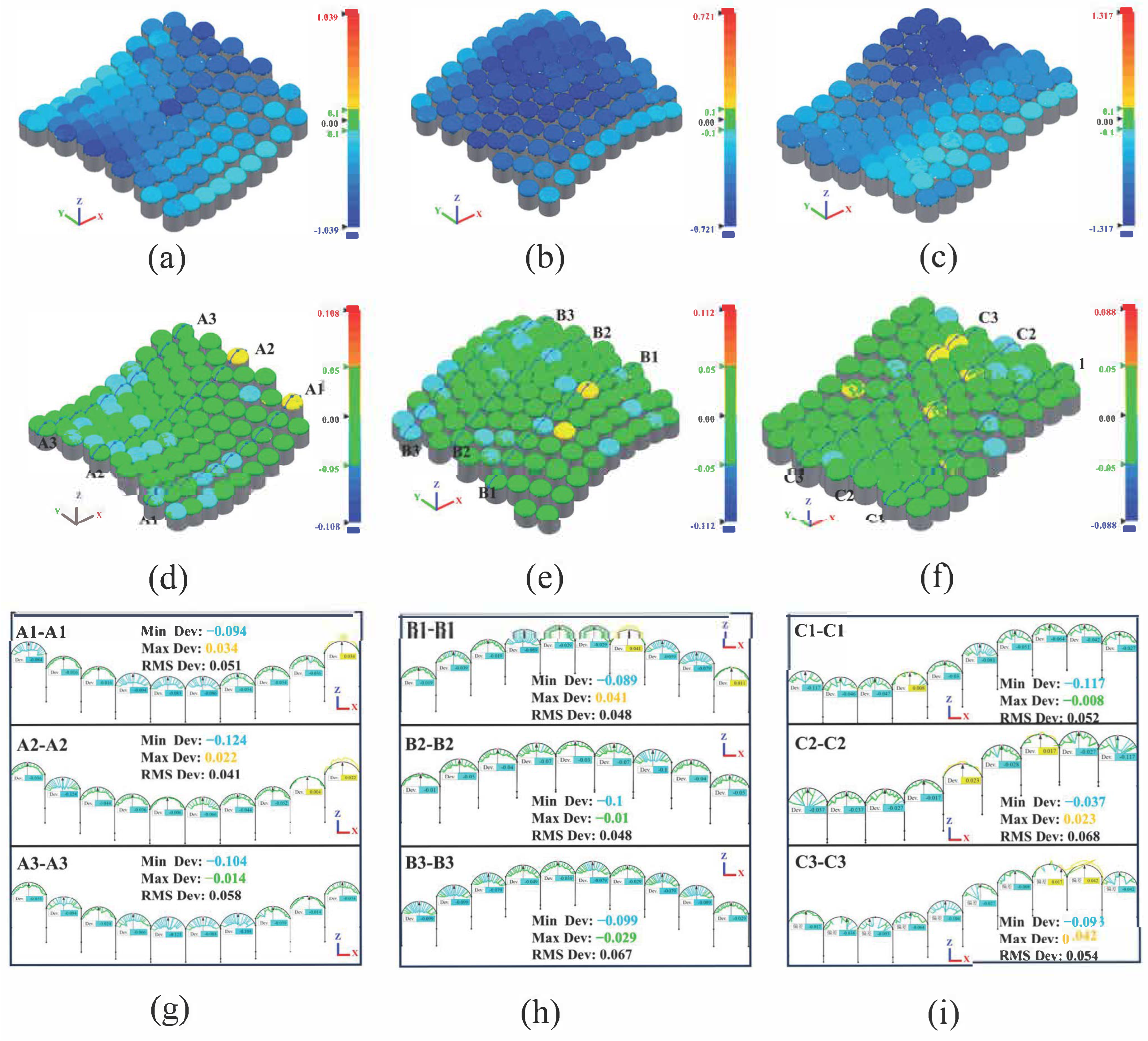
Figure 13 presents the deviation analyses of the saddle, spherical, and wavy composite surfaces before and after applying the neural network-based compensation strategy. As shown in Figure 13a–c, noticeable deviations were observed in all three surface types before compensation, with maximum errors of ±1.04 mm, ±0.72 mm, and ±1.32 mm, respectively. After compensation, Figure 13d–f, the deviation magnitudes were significantly reduced, and the error distributions became more uniform across all surfaces. The cross-sectional profiles further corroborate this improvement. For the saddle surface (A1–A3, Figure 13g), the mean deviation decreased from −0.481 mm to −0.012 mm, with the deviation range narrowed to between −0.124 mm and 0.034 mm (RMS 0.041–0.058 mm), and 82.4% of the surface falling within ±0.05 mm. The spherical surface (B1-B3, Figure 13h) exhibited a similar trend, with the mean deviation reduced from −0.485 mm to −0.010 mm, and the profiles confined between −0.100 mm and 0.041 mm (RMS 0.048–0.067 mm), achieving 84.0% conformity within the ±0.05 mm tolerance. The wavy surface (C1–C3, Figure 13i) showed the most pronounced improvement, with the mean deviation reduced from −0.492 mm to −0.030 mm and the cross-sectional deviations controlled within −0.117 mm and 0.052 mm (RMS 0.052–0.068 mm), resulting in 90.3% of the surface satisfying the ±0.05 mm tolerance threshold. The results indicate that the proposed compensation strategy effectively mitigates height deviations caused by the RAPDS when reconstructing complex composite geometries using flexible multi-point mold die support units. Moreover, the method demonstrates strong adaptability to surfaces with varying curvature and maintains stable adjustment accuracy. Overall, these findings validate the robustness and practical feasibility of the BO-ASFSSA-BPNN compensation framework integrated with the RAPDS for high-precision composite surface reconstruction.

6.3. Evaluation of the Shape Accuracy of Composite Components

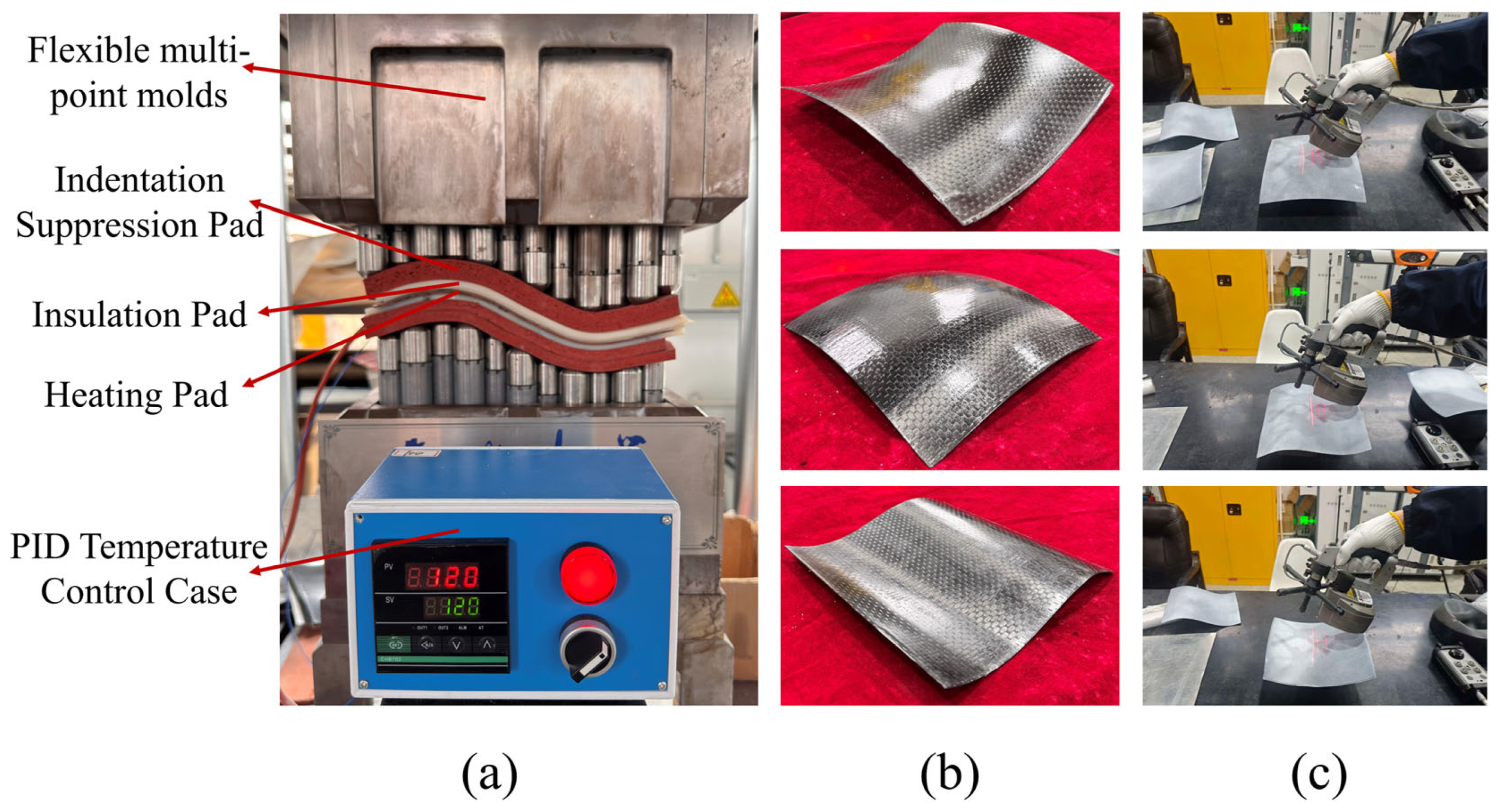
To evaluate the effectiveness of the proposed flexible multi-point mold in improving the forming accuracy and efficiency of composite components, three types of composite specimens were fabricated and analyzed, as illustrated in Figure 14. Figure 14a shows the flexible forming setup based on the MPRD, which mainly consists of multiple supporting units, a heating pad, an insulation pad, an indentation suppression pad, and a PID temperature control system. To ensure uniform heat transfer and consistent curing quality, a two-stage heating and curing scheme was applied. The temperature was first increased from room temperature to 80 °C and maintained for 90 min under a hydraulic pressure of 0.8 MPa, followed by heating to 120 °C and holding for 120 min to complete curing. Through the optimized surface adjustment and configuration process, the die surface was efficiently reshaped to the target geometry, enabling accurate and efficient forming of the composite specimens. As shown in Figure 14b, the three carbon fiber composite parts obtained from the flexible multi-point mold process exhibited smooth surfaces and well-defined geometries without noticeable defects. Subsequently, a high-precision 3D scanning system was used to capture the surface morphology of the formed parts, as shown in Figure 14c, providing the data required for the quantitative evaluation of geometric accuracy.
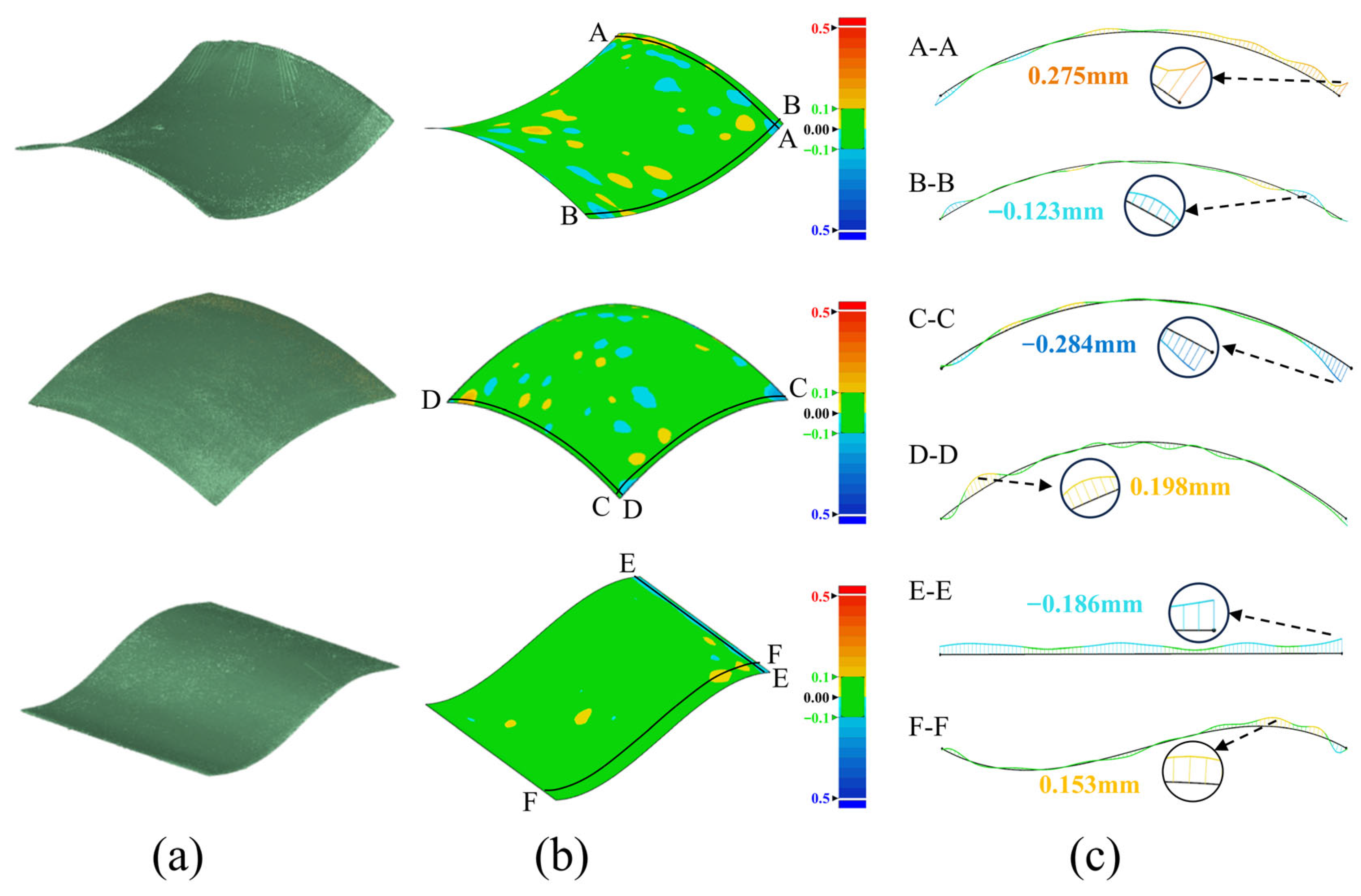
Figure 15 presents the geometric evaluation results of the three composite components obtained from the 3D scanning process shown in Figure 14c. Figure 15a shows the reconstructed point cloud models of the three formed components, while Figure 15b illustrates the corresponding overall surface deviation maps. The results indicate that more than 90.2% of the surface points of all three CFRP components fall within a deviation range of ±0.1 mm, which satisfies the typical tolerance requirements for high-precision aerospace and automotive applications. This demonstrates that the proposed flexible multi-point forming process can maintain stable geometric accuracy during continuous fabrication. Figure 15c shows the cross-sectional deviation profiles extracted from the regions with the maximum and minimum deviations identified in Figure 15b. The largest deviations mainly occur near the edges of the components, which may be attributed to resin flow during curing or slight warpage after forming. The two-dimensional sectional analysis further confirms that the formed surfaces of the three composite components closely match the designed target geometry, with only minor deviations appearing along the boundaries.

7. Conclusions

In this study, a machine-learning-based robot-assisted precision driving system (RAPDS) was developed for achieving precise actuation and adaptive error control of discrete units in flexible molds, thereby optimizing the forming process of fiber-reinforced composites (FRCs). The system integrates a backpropagation (BP) neural network, the tangential offset unit configuration (TOUC) algorithm, industrial robotic actuation, Bayesian optimization (BO), and the Adaptive Spiral Flight Sparrow Search Algorithm (ASFSSA). The main conclusions are as follows.
(1)
By integrating TOUC algorithm implemented in Rhino-Python with an industrial robot, a RAPDS was developed to efficiently and accurately convert the geometric curved surfaces of composite components into the forming curved surfaces of the flexible multi-point mold. Compared with the conventional fixed-mold manufacturing method for composite components, this system exhibits superior flexibility and adaptability in the composite forming and manufacturing process.
(2)
The proposed BO-ASFSSA-BPNN adopts a bi-level optimization framework that effectively enhances model stability, accuracy, and generalization. Compared with traditional BPNN variants, it achieves significantly lower prediction errors (RMSE = 0.0218 mm, MAE = 0.0148 mm) and a higher determination coefficient (R2 = 0.9973), providing reliable predictive support for the feedforward error compensation of the RAPDS and enabling high-precision and efficient composite forming.
(3)
The experimental results confirm that the proposed compensation strategy markedly enhances adjustment accuracy for both planar and complex composite surfaces. The maximum deviation in planar alignment was reduced from ±2.22 mm to ±0.12 mm, while over 85.0% of complex surface points fell within the ±0.05 mm tolerance. This strategy ensures stable, high-precision adjustment and significantly improves geometric conformity between the composite forming surface and the flexible multi-point mold, providing a robust basis for efficient flexible manufacturing.
(4)
The experimental results from the forming tests of composite components demonstrate that, during the continuous flexible manufacturing of three distinct complex geometries, more than 90.2% of the surface deviations of all formed components remain within ±0.1 mm. This finding confirms that the proposed flexible multi-point forming process can maintain stable geometric accuracy throughout continuous manufacturing. Moreover, the consistency and smoothness of the formed composite surfaces validate the process reliability and surface replication capability of the flexible multi-point mold.
In this study, significant improvements in the reconstruction accuracy and efficiency of surfaces within the flexible multi-point mold were achieved through the integration of the TOUC algorithm, industrial robotic execution, and the BO-ASFSSA-BPNN model. These developments establish a data-driven foundation for high-precision and efficient forming of composite components in flexible manufacturing applications. Although the current RAPDS framework demonstrates stable performance, it still operates based on a feedforward and offline optimization strategy. This limitation means that the system cannot update its compensation decisions during the forming process, and the absence of closed-loop feedback prevents it from responding to evolving deviations or unexpected disturbances in real time. Addressing this constraint is essential for extending the technology to more dynamic and variable forming scenarios. To achieve real-time operation and effectively integrate adaptive error compensation in dynamic forming environments, further in-depth research is required. Future work will focus on developing a real-time adaptive compensation framework that integrates online sensing, closed-loop feedback, and predictive modeling to further enhance the responsiveness and autonomy of the RAPDS. Moreover, the integration of the bi-level optimized neural network into intelligent manufacturing platforms will be pursued to enable in-situ learning and adaptive reconfiguration. The proposed RAPDS has strong potential to evolve into a core enabling technology for intelligent, high-precision forming and reconfigurable manufacturing of fiber-reinforced composites.

Author Contributions

W.W.: Writing—Original draft, Validation, Software, Methodology, investigation, Formal analysis, Data Curation. H.S.: Formal analysis. X.C.: Methodology. R.D.: Data Curation, J.S. and Y.L.: Investigation. X.W., S.H. and J.Y.: Data Curation. Q.H.: Writing review & editing, Supervision. All authors have read and agreed to the published version of the manuscript.

Funding

This research was funded by the National Key R&D Program of China (2021YFF0500103), the pre-production and industrialization projects of Scientific and Technological Achievements of Jilin University (23GNZ24), and Program for the Central University Youth Innovation Team (419021423505).

Data Availability Statement

The original contributions presented in this study are included in the article. Further inquiries can be directed to the corresponding author.

Conflicts of Interest

The authors declare no conflict of interest.

References

  1. Shi, M.D.; Han, Q.G.; Liu, X.; Cheng, X.H.; Han, Z.W. Coupling bionic design and application of flow curved surface for carbon fiber composite fan blade. J. Mater. Res. Technol. 2023, 27, 1797–1807. [Google Scholar] [CrossRef]
  2. He, D.; Kim, H.C.; Sommacal, S.; Stojcevski, F.; Soo, V.K.; Lipinski, W.; Morozov, E.; Henderson, L.C.; Compston, P.; Doolan, M. Improving mechanical and life cycle environmental performances of recycled CFRP automotive component by fibre architecture preservation. Compos. Part A Appl. Sci. Manuf. 2023, 175, 107749. [Google Scholar] [CrossRef]
  3. Miyano, Y.; Nakada, M.; Ichimura, J.; Hayakawa, E. Accelerated testing for long-term strength of innovative CFRP laminates for marine use. Compos. Part B Eng. 2008, 39, 5–12. [Google Scholar] [CrossRef]
  4. Zhu, Z.; Tang, X.; Chen, C.; Peng, F.; Yan, R.; Zhou, L.; Li, Z.; Wu, J. High precision and efficiency robotic milling of complex parts: Challenges, approaches and trends. Chin. J. Aeronaut. 2022, 35, 22–46. [Google Scholar] [CrossRef]
  5. Tang, Y.; Fairclough, J.P.A. A novel tooling-free carbon fibre reinforced polymer (CFRP) manufacturing method, double point incremental forming (DPIF) with direct electrical curing (DEC). Compos. Part A Appl. Sci. Manuf. 2024, 187, 108478. [Google Scholar] [CrossRef]
  6. Vita, A.; Castorani, V.; Germani, M.; Marconi, M. Comparative life cycle assessment of low-pressure RTM, compression RTM and high-pressure RTM manufacturing processes to produce CFRP car hoods. Procedia CIRP 2019, 80, 352–357. [Google Scholar] [CrossRef]
  7. Li, Y.; Shi, Z.; Rong, Q.; Zhou, W.; Lin, J. Effect of pin arrangement on formed shape with sparse multi-point flexible tool for creep age forming. Int. J. Mach. Tools Manuf. 2019, 140, 48–61. [Google Scholar] [CrossRef]
  8. Cheng, X.; Han, Q.; Huang, Y.; Shi, M.; Shi, H.; Ji, M.; Yang, C. Bioinspired ultra-fine hybrid nanocoating for improving strength and damage tolerance of composite fan blades in flexible manufacturing. Compos. Sci. Technol. 2025, 259, 110956. [Google Scholar] [CrossRef]
  9. Cai, Z.-Y.; Wang, S.-H.; Xu, X.-D.; Li, M.-Z. Numerical simulation for the multi-point stretch forming process of sheet metal. J. Mater. Process. Technol. 2009, 209, 396–407. [Google Scholar] [CrossRef]
  10. Zhang, Q.; Wang, Z.R.; Dean, T.A. The mechanics of multi-point sandwich forming. Int. J. Mach. Tools Manuf. 2008, 48, 1495–1503. [Google Scholar] [CrossRef]
  11. Qu, E.; Li, M.; Li, R. Investigation of spring-back using a discrete steel pad in multi-point forming. Int. J. Adv. Manuf. Technol. 2019, 103, 4541–4551. [Google Scholar]
  12. Liu, C.; Li, M.; Fu, W. Principles and apparatus of multi-point forming for sheet metal. Int. J. Adv. Manuf. Technol. 2008, 35, 1227–1233. [Google Scholar] [CrossRef]
  13. Jia, B.-B.; Chen, G.; Wang, W.-W.; Shen, Y.; Gu, Y. Deformation characteristics and forming force limits of multi-point forming with individually controlled force-displacement. Int. J. Adv. Manuf. Technol. 2022, 123, 1565–1576. [Google Scholar] [CrossRef]
  14. Jia, B.-B.; Shen, Y.; Gu, Y. Influence of the deformation sequence on the shape accuracy of multi-point forming. Int. J. Adv. Manuf. Technol. 2023, 16, 66. [Google Scholar] [CrossRef]
  15. Zhao, X.; Ou, H. A new flexible multi-point incremental sheet forming process with multi-layer sheets. J. Mater. Process. Technol. 2023, 322, 118214. [Google Scholar] [CrossRef]
  16. Zheng, S.; El-Aty, A.A.; Hu, S.; Cui, Z.; Lu, Y.; Liu, C.; Cheng, C.; Tao, J.; Guo, X. Innovative high degree of freedom single-multipoint incremental forming system for manufacturing curved thin-walled components. J. Manuf. Syst. 2024, 74, 1019–1036. [Google Scholar] [CrossRef]
  17. Zheng, Y.; Liu, W.; Zhang, Y.; Han, L.; Li, J.; Lu, Y. Integration and calibration of an in situ robotic manufacturing system for high-precision machining of large-span spacecraft brackets with associated datum. Robot. Comput. Integr. Manuf. 2025, 94, 102928. [Google Scholar] [CrossRef]
  18. Choi, Y.W.; Lee, J.; Lee, Y.; Lee, S.; Jeong, W.; Lim, D.Y.; Lee, S.W. A vision-guided adaptive and optimized robotic fabric gripping system for garment manufacturing automation. Robot. Comput. Integr. Manuf. 2025, 92, 102874. [Google Scholar] [CrossRef]
  19. Song, C.; Liu, Z.; Wang, X.; Qiu, T.; Liang, Z.; Shen, W.; Gao, Y.; Ma, S. Surface roughness online prediction using parallel ensemble learning in robotic side milling for aluminum alloy. Mech. Syst. Signal Process. 2025, 235, 112932. [Google Scholar] [CrossRef]
  20. Zhang, J.; Zou, L.; Zhang, X.; Wang, Z.; Wang, W. An error compensation method for on-machine measuring blade with industrial robot. Measurement 2025, 242, 116039. [Google Scholar] [CrossRef]
  21. Ma, W.; Hu, T.; Zhang, C.; Chen, Q. Adaptive remanufacturing for freeform surface parts based on linear laser scanner and robotic laser cladding. Robot. Comput. Integr. Manuf. 2025, 91, 102855. [Google Scholar] [CrossRef]
  22. Wu, C.; Guo, K.; Sun, J.; Liu, Y.; Zheng, D. Active vibration control in robotic grinding using six-axis acceleration feedback. Mech. Syst. Signal Process. 2024, 214, 111379. [Google Scholar] [CrossRef]
  23. Chen, C.; Cai, Z.; Chen, T.; Li, Z.; Yang, F.; Liang, X. A vision-based calibration method for aero-engine blade-robotic grinding system. Int. J. Adv. Manuf. Technol. 2023, 125, 2195–2209. [Google Scholar] [CrossRef]
  24. Cai, Z.-Y.; Li, M.-Z. Multi-point forming of three-dimensional sheet metal and the control of the forming process. Int. J. Press. Ves. Pip. 2002, 79, 289–296. [Google Scholar] [CrossRef]
  25. Cai, Z.; Li, M. Optimum path forming technique for sheet metal and its realization in multi-point forming. J. Mater. Process. Technol. 2001, 110, 136–141. [Google Scholar]
  26. Tan, F.X.; Li, M.Z.; Cai, Z.Y. Research on the process of multi-point forming for the customized titanium alloy cranial prosthesis. J. Mater. Process. Technol. 2007, 187–188, 453–457. [Google Scholar] [CrossRef]
  27. Xiao, Y.; Zhou, X.; Zhou, H.; Wang, J. Multi-label deep transfer learning method for coupling fault diagnosis. Mech. Syst. Signal Process. 2024, 212, 111327. [Google Scholar] [CrossRef]
  28. Zhou, Z.; Li, L.; Fürsterling, A.; Durocher, H.J.; Mouridsen, J.; Zhang, X. Learning-based object detection and localization for a mobile robot manipulator in SME production. Robot. Comput. Integr. Manuf. 2022, 73, 102229. [Google Scholar] [CrossRef]
  29. Zheng, Y.; Liu, W.; Zhang, Y.; Ding, H.; Li, J.; Lu, Y. Laser in-situ measurement in robotic machining of large-area complex parts. Measurement 2025, 241, 115718. [Google Scholar] [CrossRef]
  30. Gong, J.; Song, Q.; Fu, H.; Jiang, L.; Zhang, H.; Cai, Y.; Liu, Z.; Luan, Q.; Wang, H. Systematic error reduction in laser triangulation OMM: A study on measurement parameters and compensation techniques. Measurement 2025, 247, 116802. [Google Scholar] [CrossRef]
  31. Li, F.; Wu, Z.; Qian, F.; Yue, T.; Xu, T. Adaptive active noise feedforward compensation for exhaust ducts using a FIR Youla parametrization. Mech. Syst. Signal Process. 2022, 170, 108803. [Google Scholar] [CrossRef]
  32. Lei, Y.; Yang, B.; Jiang, X.; Jia, F.; Li, N.; Nandi, A.K. Applications of machine learning to machine fault diagnosis: A review and roadmap. Mech. Syst. Signal Process. 2020, 138, 106587. [Google Scholar] [CrossRef]
  33. Liu, Y.; Zhao, Y.; Lin, Q.; Pan, W.; Wang, W.; Ge, E. DeviationGAN: A generative end-to-end approach for the deviation prediction of sheet metal assembly. Mech. Syst. Signal Process. 2023, 204, 110822. [Google Scholar] [CrossRef]
  34. Ma, Q.; Yue, C.; Yu, M.; Song, Y.; Cui, P.; Yu, Y. Research on fault diagnosis strategy of air-conditioning system based on signal demodulation and BPNN-PCA. Int. J. Refrig. 2024, 158, 124–134. [Google Scholar] [CrossRef]
  35. Yang, X.; Xie, L.; Chen, J.; Zhao, B.; Wang, K. Estimation of Weibull distribution using the back-propagation neural network for fatigue failure data. Probabilistic Eng. Mech. 2025, 82, 103828. [Google Scholar] [CrossRef]
  36. Kang, R.; Hu, J.; Li, M.; Zhang, Q.; Su, X.; Li, Z.; Tian, W. Digital twin modeling of the robotic gluing system for predicting the quality of glue lines and optimizing gluing parameters. J. Manuf. Syst. 2025, 80, 1074–1092. [Google Scholar] [CrossRef]
  37. Wang, Y.; Ge, Q. Adaptive STCPF for UCA pose estimation with improved GA-BPNN and multiple fading factors. Neurocomputing 2024, 575, 127238. [Google Scholar] [CrossRef]
  38. Chen, G.; Liu, M.; Chen, J. Frequency-temporal-logic-based bearing fault diagnosis and fault interpretation using Bayesian optimization with Bayesian neural networks. Mech. Syst. Signal Process. 2020, 145, 106951. [Google Scholar] [CrossRef]
  39. Shi, H.; Wang, W.; Cheng, X.; Sun, J.; Ding, R.; Yue, D.; Han, Q. Curvature-driven regionally sampling and machine learning for forming error measurement in composite manufacturing. Mech. Syst. Signal Process. 2025, 238, 113231. [Google Scholar] [CrossRef]
  40. Sun, J.; Han, Q.; Cheng, X.; Shi, H.; Ding, R.; Shi, M.; Liu, C. A data-driven computational optimization framework for designing thin-walled lenticular deployable composite boom with optimal load-bearing and folding capabilities. Thin-Walled Struct. 2024, 203, 112244. [Google Scholar] [CrossRef]
  41. Ouyang, C.; Qiu, Y.; Zhu, D. Adaptive Spiral Flying Sparrow Search Algorithm. Sci. Program. 2021, 2021, 6505253. [Google Scholar] [CrossRef]
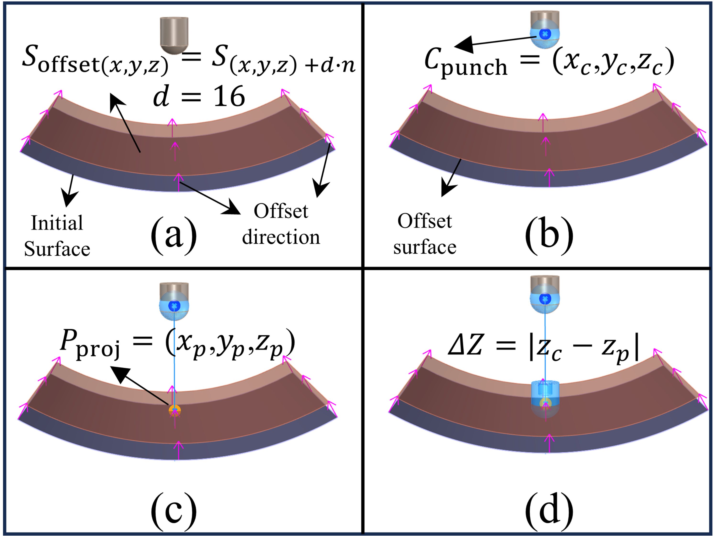
Figure 1. Tangential Offset Unit Configuration Algorithm: (a). Offset surface generation along unit normal vectors, (b). Spherical fitting of the punch tip to locate the punch center, (c). Z-directional projection of the fitted center onto the offset surface, (d). Computation of vertical displacement (ΔZ) for achieving tangential alignment.
Eng 06 00356 g001
Figure 2. RAPDS for composite surface reconstruction process.
Eng 06 00356 g002
Figure 3. Laser-based robotic system for measuring errors in multi-point flexible forming molds.
Eng 06 00356 g003
Figure 4. Correlation analysis of adjustment errors in RAPDS.
Eng 06 00356 g004
Figure 5. Response surface methodology for RAPDS adjustment error prediction: (a1a3). Experimental setup and implementation, (b1b3). 3D interaction surfaces, (c1c3). model prediction performance.
Eng 06 00356 g005
Figure 6. Neural network architecture for adjustment error prediction.
Eng 06 00356 g006
Figure 7. Bi-level optimization of BPNN for RAPDS adjustment error prediction. (a). Bayesian hyperparameter tuning, (b). ASFSSA-based weight and threshold optimization.
Eng 06 00356 g007
Figure 8. Comparative results of four BPNN-based models: (a1a4). predicted vs. actual, (b1b4). residual surfaces, (c1c4). test-set error trends.
Eng 06 00356 g008
Figure 9. Experimental procedure of the error compensation method: (a). theoretical calculation of composite curves, (b). machine learning prediction, (c). measurement of initial plane error, (d). robot-assisted precision driving.
Eng 06 00356 g009
Figure 10. High-precision 3D scanning and measurement device.
Eng 06 00356 g010
Figure 11. Surface error compensation in initial plane alignment: (a) initial errors (b) predicted errors, (c) compensation value (d) final errors after adjustment.
Eng 06 00356 g011
Figure 12. 3D complex surfaces of flexible multi-point mold and their corresponding point clouds.
Eng 06 00356 g012
Figure 13. 3D point-cloud and 2D cross-sectional deviation analysis of saddle, spherical and wavy surfaces before and after BO-ASFSSA-BPNN compensation: (ac) pre-compensation 3D deviations, (df). post-compensation 3D deviations, (gi) 2D cross-sectional profiles along the A-A, B-B and C-C series lines.
Eng 06 00356 g013
Figure 14. Flexible forming and 3D scanning of composite parts: (a) forming setup, (b) formed components, (c) 3D scanning process.
Eng 06 00356 g014
Figure 15. Geometric deviation analysis of the three formed composite components: (a) measure point cloud, (b) shape error cloud maps, (c) local error curve.
Eng 06 00356 g015
Table 1. Box–Behnken design matrix for six-factor RAPDS analysis.
RunX1 (mm)X2 (mm)X3X4 (°C)X5 (mm)X6Y (mm)
10.0293.67104.0020.000.004.000.31
2100.0015.0052.0023.000.003.001.56
3100.0093.671.0020.000.002.001.67
450.01176.84104.0020.00−1.503.001.03
550.0193.6752.0020.000.003.000.73
6100.0093.6752.0017.001.503.001.55
750.0193.6752.0020.000.003.000.77
8100.0093.6752.0017.00−1.503.001.53
950.0115.001.0020.00−1.503.000.33
1050.0115.0052.0020.00−1.504.000.59
1150.0115.001.0020.001.503.000.32
1250.0193.671.0017.000.002.000.26
130.0293.671.0020.000.002.000.04
1450.0193.67104.0017.000.002.001.88
1550.0115.00104.0020.00−1.503.000.77
160.0215.0052.0017.000.003.000.23
1750.0193.67104.0023.000.004.001.89
1850.0193.6752.0020.000.003.000.53
1950.01176.841.0020.001.503.000.61
2050.0115.00104.0020.001.503.000.98
2150.0115.0052.0020.00−1.502.000.53
220.0293.6752.0017.001.503.000.21
2350.0193.671.0023.000.004.000.21
240.0293.67104.0020.000.002.000.46
25100.093.6752.0023.00−1.503.001.33
2650.01176.84104.0020.001.503.001.37
2750.01176.8452.0020.001.502.000.71
2850.0193.6752.0020.000.003.000.62
2950.01176.8452.0020.00−1.502.000.88
300.02176.8452.0023.000.003.000.47
310.0293.671.0020.000.004.000.02
3250.01176.841.0020.00−1.503.000.99
3350.0115.0052.0020.001.502.000.71
34100.00176.8452.0017.000.003.001.44
35100.0015.0052.0017.000.003.001.55
3650.0193.67104.0017.000.004.001.73
3750.0193.6752.0020.000.003.000.66
380.0293.6752.0017.00−1.503.000.19
390.0293.6752.0023.00−1.503.000.26
4050.0193.671.0017.000.004.000.45
410.0293.6752.0023.001.503.001.33
42100.0093.6752.0023.001.503.001.47
430.0215.0052.0023.000.003.000.03
4450.01176.8452.0020.001.504.000.91
45100.0093.67104.0020.000.004.001.46
46100.00176.8452.0023.000.003.001.77
4750.0193.67104.0023.000.002.001.76
4850.0115.0052.0020.001.504.000.73
49100.0093.671.0020.000.004.001.01
500.02176.8452.0017.000.003.000.49
5150.01176.8452.0020.00−1.504.000.83
5250.0193.6752.0020.000.003.000.79
53100.0093.67104.0020.000.002.001.85
5450.0193.671.0023.000.002.000.44
Table 2. Statistical screening of factors influencing adjustment error.
FactorPCC (r)SRC (ρ)F-Valuep-Value
Theoretical Height (mm)0.6630.63663.7220.001
Radial Distance (mm)0.1780.1854.2100.050
Adjustment Sequence0.2470.28434.9610.001
Ambient Temperature (°C)−0.050−0.0400.4540.507
Initial Error (mm)0.0890.0731.1430.295
Motor Speed Level0.0650.0590.4540.504
Table 3. Performance comparison of different BPNN models for adjustment error prediction.
ModelsR2RMSEMAEMAPETraining Time/s
BPNN0.90890.11120.085912.4%2.00
BO-BPNN0.95040.04680.03586.6%4.19
ASFSSA-BPNN0.96990.03720.02564.4%20.00
BO-ASFSSA-BPNN0.99730.02180.01482.2%16.14
Disclaimer/Publisher’s Note: The statements, opinions and data contained in all publications are solely those of the individual author(s) and contributor(s) and not of MDPI and/or the editor(s). MDPI and/or the editor(s) disclaim responsibility for any injury to people or property resulting from any ideas, methods, instructions or products referred to in the content.