An Integrated TCN-GRU Deep Learning Approach for Fault Detection in Floating Offshore Wind Turbine Drivetrains

Abstract

In the complex operational environment of offshore wind turbines, the drivetrain system faces multiple uncertainties including wind speed fluctuations, wave disturbances, and dynamic coupling effects, which significantly increase the difficulty of fault identification. To address this challenge, this paper proposes a deep learning model integrating Temporal Convolutional Networks (TCN) and Gated Recurrent Units (GRU) to enhance fault detection capability. The TCN module extracts multi-scale temporal features from vibration signals, while the GRU module captures long-term dependencies in drivetrain degradation patterns. The study utilizes a publicly available Zenodo dataset containing simulated acceleration signals from a 5-MW reference drivetrain under three offshore conditions, covering healthy and faulty states of the main shaft, high-speed shaft, and planet bearings. Experimental validation under different operational conditions demonstrates that the proposed TCN-GRU model outperforms baseline models in terms of accuracy, precision, and recall.

1. Introduction

In recent years, offshore wind energy technology has continuously evolved. Floating wind turbines, which are unaffected by seabed geological conditions, have demonstrated significant potential for deployment in deep-sea regions. However, due to their extended operation in complex marine environments, floating wind turbines face greater challenges regarding operational stability and maintenance. The drivetrain, as a critical power transmission component in wind turbines, is subject to a relatively high failure rate compared to other subsystems. Issues such as gear wear, bearing damage, or inadequate lubrication not only result in equipment downtime but also incur substantial repair costs. This is especially problematic in offshore locations, where maintenance is particularly challenging. As a result, there is an urgent need to develop efficient and intelligent fault detection methods for drivetrain systems [1,2,3].

Early fault detection in the drivetrain system is crucial for the stable operation of wind turbines and for reducing maintenance costs [4]. Especially in floating offshore wind turbines, the complexity of the offshore environment presents additional challenges for fault detection [5]. Accurate and efficient fault detection can significantly enhance the system reliability. Research by Musial et al. indicates that faults in the wind turbine drivetrain system typically originate from bearings. Therefore, early fault detection of drivetrain bearing components is particularly critical [6,7]. Similarly, by monitoring changes in the system response, the condition of the gearbox can be effectively assessed to detect early-stage faults.

In the study of fault detection for wind turbine drivetrain systems, vibration analysis [8] and oil analysis [9,10] are the commonly employed technical approaches. Of these, vibration-based condition monitoring has become one of the standard methods for drivetrain fault detection [11]. This approach leverages the fact that system defects induce rapid changes in vibration signals [12]. Standards such as ISO 10816-21 [13] and ISO 16079-2 [14] provide explicit recommendations for critical measurement locations in drivetrain vibration monitoring. These measurement points are typically situated close to components with high failure rates, such as bearings and gears, to promptly capture signal variations induced by faults. Thus, optimizing the placement of vibration sensors on the drivetrain to minimize sensor count while preserving adequate fault-related data is critical for improving the efficiency and economic viability of fault detection [15]. To determine the optimal placement and number of vibration sensors, it is first necessary to investigate the complex relationships among the signals from various sensors. A system health function can be constructed based on the shared information among multiple sensors. When a fault occurs, this shared information changes [16], thereby altering the health function. For example, many studies have used the degree of correlation between vibration measurements as a fault indicator in the detection of rotating machinery. Xiong et al. [17] also developed a fault detection method for rotating machinery that integrates dimensionless indicators with the Pearson correlation coefficient. However, traditional methods based on correlation analysis exhibit limitations in handling high-dimensional, multi-source, and nonlinear data and thus cannot fully capture complex fault characteristics.

With the advancement of information technology and breakthroughs in deep learning, data-driven fault detection methods have been widely applied in the field of wind turbines. Zare and Ayati [18] developed a fault detection algorithm based on a self-constructed database using a multi-channel convolutional neural network (CNN). In their study, multiple fault types, such as rotor imbalance and pitch actuator faults, were simulated in a 5 MW wind turbine benchmark model, and high diagnostic accuracy was achieved under various wind speed conditions. Ziane et al. [19] proposed neural network optimization algorithms to predict the fatigue life of wind turbine blades under variable hygrothermal conditions, employing multiple metaheuristic approaches to improve prediction accuracy. Garousi et al. [20] performed vibration analysis of centrifugal pumps with healthy and defective impellers, using a multi-layer perceptron (MLP) algorithm to detect and classify faults based on features in the time and frequency domains. Cui et al. [21] employed a recurrent neural network (RNN) to capture long-term temporal dependencies among various time-series signals, and their results indicated that the model successfully identified operational risks and decreased false alarms. Recently, more advanced architectures have been explored to address the challenges in wind turbine fault detection. Xiang et al. [22] developed a fault detection model for wind turbines using SCADA data by combining convolutional neural networks (CNN) and long short-term memory (LSTM) with an attention mechanism. This hybrid deep learning framework effectively captures spatial–temporal dependencies in multivariate sensor data and enhances the accuracy and interpretability of fault detection. Wang et al. [23] developed a hybrid model combining one-dimensional CNN with bidirectional LSTM (1D-CNN-BiLSTM) for multi-fault detection of wind turbine gearboxes, demonstrating superior performance in feature extraction and temporal modeling compared to traditional methods. More recently, Chen et al. [24] proposed a transfer learning–based framework for wind turbine fault diagnosis by integrating Inception V3 and TrAdaBoost algorithms to identify blade icing and gear cog belt fracture using SCADA data. Despite these significant advances in fault detection accuracy and modeling techniques, existing studies still exhibit certain limitations including heavy reliance on large-scale labeled data, limited generalization capability across different operating conditions, insufficient real-time performance for online monitoring, and challenges in adapting to the complex and dynamic marine environments of offshore wind farms.

Existing studies on drivetrain fault diagnosis fall into two main categories: (i) data-driven approaches using experimental or SCADA measurements, exemplified by Hamid et al. [25] who developed a CNN-based method for bearing-fault identification in high-speed wind turbines and by Teng et al. [26] who conducted a comprehensive vibration-analysis investigation for drivetrain fault detection, and (ii) approaches based on physics-based simulation models. The methods rely on real measurement data, which contain realistic noise and operational variability but suffer from incomplete labeling, limited fault types, and the difficulty of obtaining representative fault samples from operating turbines. In contrast, the present study employs a model-based simulation framework, where diverse fault scenarios are generated using a validated multibody dynamics model. This enables full control over operating conditions, reproducible fault cases, and complete fault labeling, providing a systematic benchmark for the development and evaluation of deep learning-based diagnostic methods. Therefore, the proposed work complements existing experimental and SCADA-based studies by offering a controlled simulation platform for early-stage algorithm validation.

Addressing the identified challenges, this study aims to fulfill the stringent fault detection demands of floating offshore wind turbine drivetrain systems operating under intricate and dynamic marine conditions. To tackle the complexities arising from time-varying loads, multi-coupling vibrations, and non-stationary operational states, an improved deep learning framework is proposed that synergistically combines Temporal Convolutional Networks (TCN) with Gated Recurrent Units (GRU). In this hybrid architecture, the complementary strengths of both networks are strategically leveraged: TCN excels in capturing long-range dependencies through dilated causal convolutions and parallel processing, while GRU demonstrates superior capability in modeling non-linear dynamics and sequential patterns inherent in vibration signals. Furthermore, to address the high dimensionality and redundancy issues in multi-sensor monitoring data, the Pearson correlation coefficient is incorporated as a feature selection criterion and enables effective dimensionality reduction while preserving critical diagnostic information. This integrated approach not only enhances the diagnostic accuracy by extracting more discriminative fault features from complex signal patterns, but also significantly improves the real-time performance and computational efficiency of the model. These improvements make it particularly suitable for online condition monitoring applications in offshore wind farms. The proposed methodology demonstrates strong potential for practical deployment in harsh marine environments where reliability and timely fault detection are paramount.

The remainder of this paper is organized as follows. Section 2 introduces the wind turbine and drivetrain model used in this study, the decoupled analysis method applied to obtain drivetrain loads, and the defined fault scenarios. Section 3 elaborates on the methodology employed, including data preprocessing, Pearson correlation analysis and the architecture of the proposed model. Section 4 presents the experimental results and provides an in-depth discussion. Finally, Section 5 concludes the paper and outlines prospects for future research.

2. Numerical Models

2.1. Wind Turbine Reference Model

The OC3-Hywind Spar-type 5 MW floating wind turbine [27] is adopted as the reference model in this study. The mooring system of the Spar-type platform is typically composed of mooring cables or chains. Compared to other floating foundations, advantages such as a simpler structure, lower installation costs, and reduced wave-induced motions are offered, which makes it more suitable for deployment in deep-water regions. The main parameters of the Spar-type floating wind turbine and the key characteristics of its platform are summarized in

Table 1. NREL 5MW Spar Wind Turbine System-Complete Specifications.

System Parameters
Wind Turbine
	Rated power	5 MW
	Number of blades	3
	Rotor/hub diameter	126 m/3 m
	Hub height	90 m
	Operating wind speed	3–25 m/s (rated: 11.4 m/s)
	Masses (rotor/nacelle/tower)	110/240/347.46 t
Spar Platform
	Mooring lines	3
	Depth to base	120 m
	Cable stiffness	$3.842\times {10}^8$ N
	Platform mass	$7.466\times {10}^6$ kg
	Roll inertia about CM	$4.229\times {10}^9$ kg/m2
Gearbox
	Configuration	2 Planetary + 1 Parallel
	Gear ratios	1:3.947/1:6.167/1:3.958
	Total ratio	1:96.354
	Designed power	5000 kW

.

2.2. Drivetrain Model and Fault Modeling

To validate the proposed fault detection method, the publicly available bearing damage dataset released by Dibaj and Nejad on Zenodo [28] was used. The dataset contains simulated acceleration signals of a 5-MW reference drivetrain on a spar-type floating wind turbine, generated with a validated SIMPACK multibody dynamics model [27]. It provides vibration data for multiple bearing fault scenarios under three representative offshore environmental conditions. The drivetrain model employed for data generation is based on the experimentally validated SIMPACK gearbox model developed by Nejad et al., and the environmental parameters were adopted from their floating wind turbine load analysis study [29]. As a result, the vibration signals utilized in this work originate from a rigorously validated simulation framework, offering reliable benchmark data for developing and assessing fault diagnosis algorithms. Although simulated data cannot fully replicate real measurements, its controllability, repeatability, and complete labeling make it highly suitable for the algorithm development stage. This reference gearbox model is installed on a Spar-type floating wind turbine. In wind turbines, a typical design is represented by the gearbox, which is comprised of three gear stages: two planetary gears and one parallel-stage gear. A four-point support configuration with two main bearings was adopted to limit non-torque loads entering the gearbox. In this reference model, the bearings are modeled using SIMPACK [30] force elements with corresponding stiffness values. The detailed parameters of the gearbox are summarized in Table 1.

The complexity of the marine environment presents greater challenges to the steady-state operation of wind turbines. Additional dynamic loads on the drivetrain are introduced by the interaction between the floating platform and marine waves, which results in increased irregularity and complexity in vibration patterns. In this study, fault scenarios are considered in the main bearing, high-speed shaft, and planetary bearings [31].

Acceleration vibration data in both axial and radial directions are acquired under three distinct environmental conditions, namely wind speeds below, at, and above the rated value. These data are used to validate the effectiveness of the model under varying operational environments. The specific environmental conditions are summarized in

Table 2. Environmental conditions.

Parameter	EC1 (Below-Rated)	EC2 (Rated)	EC3 (Above-Rated)
Wind speed U (m/s)	7.0	12.0	14.0
Turbulence intensity I (-)	0.19	0.15	0.14
Significant wave height Hs (m)	4.5	5.0	4.0
Spectral peak period Tp (s)	12.0	12.0	10.0

, with each condition corresponding to a different region on the wind turbine power curve. At below-rated wind speeds, which cover the range between the cut-in and rated wind speeds, the generator torque is regulated to optimize power output across varying wind conditions. At the rated wind speed, maximum power output within rated capacity is achieved, and blade angle adjustments are performed by the pitch control system to respond to turbulent wind conditions. Above the rated wind speed, i.e., between the rated and cut-out wind speeds, pitch control adjustments are applied to maintain power generation at the rated level. The simulation is conducted with a sampling rate of 200 Hz and a duration of 3600 s to generate acceleration signals. Forces and torques obtained from the SIMO–RIFLEX–AeroDyn simulation tools [32] are used as input to the multibody system (MBS) model of the drivetrain. Axial and radial acceleration measurements acquired from the main shaft, low-speed shaft, intermediate-speed shaft, and high-speed shaft were regarded as condition monitoring data for fault detection. Since the bearing housings are not modeled in this drivetrain system, acceleration measurements from the shaft bodies (the components closest to the bearing elements) in the MBS model are selected as condition monitoring data. Figure 1 illustrates the four specific measurement locations within the drivetrain model. These four locations are designated as MSI (Main Shaft Input), LAS (Low Speed Axis, corresponding to the planet carrier PLC), ISA (Intermediate Speed Axis), and HAS (High Speed Axis). The MSI is located on the main shaft and supported by bearings INP-A and INP-B. The LAS is positioned at the output end of the first-stage planetary gear and supported by bearings PLC-A and PLC-B. The ISA is situated on the intermediate-speed shaft following the second-stage output and supported by bearings IMS-A, B, and C. The HAS is located on the high-speed shaft after the third-stage output, supported by bearings HS-A, B, and C, and connected to the generator. Acceleration signals are acquired from the shaft body at positions near the bearing elements to capture the vibration characteristics induced by bearing faults.

Table 3. Drivetrain fault cases and corresponding stiffness values.

Fault Case	Description	Original (N/m)	Reduced (N/m)
class 0	Reference case (healthy)	–	–
class 1	Damage in main bearing (INP-B)	$4.06\times {10}^6$	$4.06\times {10}^7$
class 2	Damage in high-speed shaft bearing (HS-A)	$8.2\times {10}^8$	$8.2\times {10}^6$
class 3	Damage in low-speed planet bearing (IMS-PL-A)	$6.12\times {10}^7$	$6.12\times {10}^5$

presents the original stiffness values and reduced stiffness values for each load condition. The technical specifications of the vibration data acquisition were summarized in

Table 4. Technical specifications of the vibration data acquisition system.

Specification Item	Details
Measurement Type	Acceleration (Axial and Radial)
Sampling Frequency	200 $\mathrm{Hz}$
Signal Duration	1 h per simulation (3600 s)
Total Points per Channel	720,000 points
Data Format	MATLAB R2024b (.mat) file
Channel Configuration	4 positions × 2 directions (Axial/Radial)

. For each simulation, an acceleration time series was generated under a specific combination of fault conditions and environmental scenarios. The complete dataset provides labeled vibration signals that support fault classification tasks.

2.3. Limitations of Simulation-Based Data

In machine-learning–driven fault diagnosis, the quality and representativeness of the underlying data play a decisive role in determining the robustness, applicability, and generalization capability of the developed algorithms. In this study, the proposed method is evaluated using vibration data generated from a SIMPACK multibody dynamics model. Although simulation-based data provide several clear advantages—such as high controllability, complete labeling of fault states, and excellent repeatability—they are inevitably accompanied by a number of inherent assumptions and limitations. These factors need to be acknowledged in order to correctly interpret the diagnostic performance and to guide future research toward real-world validation.

(1)

Simplification of physical processes.

The multibody dynamics model adopted in the simulations simplifies several complex physical mechanisms to improve computational efficiency. Nonlinear material behavior inside bearings, microscopic frictional interactions, and the dynamic characteristics of lubricant films are typically approximated. Such simplifications may lead to deviations in high-frequency vibration components or transient responses when compared with actual drivetrain systems. Furthermore, fine-scale gear-mesh contact dynamics and the frequency-dependent behavior of structural damping cannot be fully represented in the current modeling framework.

(2)

Idealized measurement conditions.

In operational offshore wind turbines, vibration sensors are exposed to a variety of disturbances, including wave-induced vibrations, wind-excited structural responses, electromagnetic interference from power electronic devices, temperature variations, and sensor nonlinearities. Only a subset of these effects can be realistically incorporated into the simulated signals. As a result, diagnostic algorithms that perform well under idealized conditions may experience degradation when applied to noisy, harsh offshore environments where signal distortion, saturation, or intermittent sensor failures are common.

(3)

Absence of long-term operational effects.

Real drivetrains undergo continuous evolution during long-term operation, driven by lubricant degradation, seal aging, accumulated manufacturing tolerances, progressive gear wear, and environmental corrosion. These gradual changes alter baseline vibration characteristics and significantly influence the manifestation of fault signatures. However, the simulation data used in this study rely on snapshot-style fault representations, which do not fully capture fault progression or its coupling with system-level degradation mechanisms.

(4)

Limited representation of extreme operating conditions.

Although the dataset used in this work covers three representative environmental conditions, it still provides only a limited approximation of the highly complex offshore operating environment. Extreme wind gusts during storms or typhoons, icing and low-temperature effects, non-Gaussian and highly stochastic wave loads, and multi-factor coupled wind–wave–current interactions are not fully modeled. These extreme or atypical conditions may generate vibration responses that differ substantially from those present in the simulation scenarios, potentially constraining the generalization ability of the diagnostic algorithms.

Overall, while simulation-based data offer a valuable and well-controlled foundation for early-stage algorithm development and benchmarking, the above limitations highlight the need for future validation using real-world measurement data. Such validation will be essential to ensure the robustness and practical applicability of the proposed diagnostic framework under realistic offshore operating conditions.

3. Methodology

An end-to-end deep learning framework is employed in this study for fault diagnosis. The TCN–GRU network is used to automatically learn the mapping from vibration signals to fault categories in a purely data-driven manner. This end-to-end learning paradigm enables the extraction of complex nonlinear features and temporal dependencies, making it particularly suitable for diagnosing faults in floating offshore wind turbines and other highly coupled dynamic systems. Specifically, the input vibration signals are processed by the TCN to extract temporal features, while the GRU layer models long-term dependencies. The resulting representations are then mapped to fault classes through fully connected layers, and a probability distribution over the possible fault states is produced as the final output.

3.1. Data Preprocessing

This paper uses SIMPACK software [30] to generate simulated fault data for the 5 MW drivetrain system. This simulated data stream, which replicates the sampling characteristics of a real-time condition monitoring system, is used to train and evaluate the proposed fault diagnosis model. To ensure the reliability of the data-driven method and accurate fault detection, the dataset is divided into training and test sets, with 80% of the data (6400 samples) used for training and 20% (1600 samples) for testing. To ensure each fault type has enough training samples, the data is evenly distributed by fault type. Each category contains 2000 samples, with 1600 samples for the training set and 400 samples for the test set. During the data preprocessing, each 1-h measurement is segmented into 10-s signals, with each signal containing 2000 samples. The data from each axial and radial direction is divided into 360 signal segments to ensure the model captures sufficient feature information. All data is standardized and augmented to ensure data consistency and diversity, reducing the risk of overfitting the model.

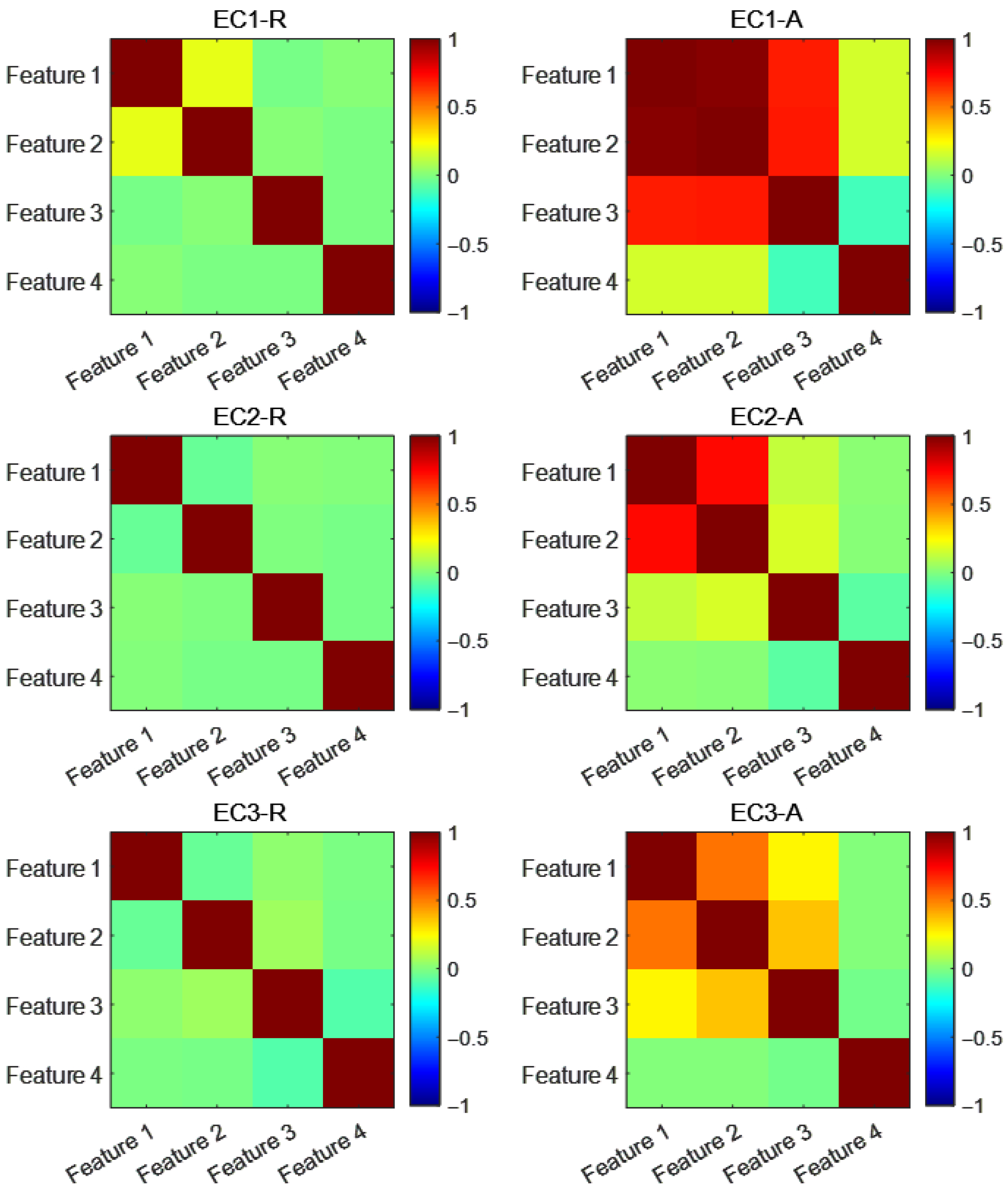
3.2. Pearson-Based Feature Analysis

For this work, the measurement values simulated by SIMPACK software are divided into training and test samples, and key features are identified through Pearson correlation analysis for constructing the fault detection model. The measured values are subjected to skin depth frequency analysis after acquisition, and a pattern recognition model for this study was established. The training data samples and test data samples are obtained through this method. The degree of linear correlation between variables was verified through quantitative analysis. Pearson Correlation Coefficient is used to provide a specific basis for feature selection. The Pearson correlation coefficient derived from Karl Pearson’s statistics is theoretically complete and computationally simple [33]. It has important applications in academic research and practical implementation. The Pearson correlation coefficient is used to measure the linear correlation between two variables. The degree of correlation between the two variables is quantified by a numerical value. The formula for the correlation coefficient is:

$$r={\displaystyle \frac{{\sum }_{i=1}^n(x_i-\overline{x})(y_i-\overline{y})}{\sqrt{{\sum }_{i=1}^n{(x_i-\overline{x})}^2}\sqrt{{\sum }_{i=1}^n{(y_i-\overline{y})}^2}}}$$

(1)

where, x and y represent the mean values of n test values, respectively. r represents the correlation coefficient between the corresponding values of 1. A positive value indicates a positive correlation. A negative value indicates a negative correlation. 0 indicates no linear correlation.

In the feature analysis, the correlation coefficient between each input feature and the output is first calculated and calculated. The predictive ability of each feature for different types of faults is evaluated based on this. The absolute value of the correlation coefficient directly reflects the importance of the feature. After the correlation coefficient is constructed, if the correlation coefficient matrix exhibited high correlation, multicollinearity issues would exist at this time. The selection and removal of features are then based on the correlation coefficient analysis results.

The final dataset is divided into training and test sets. 80% of the data (6400 samples) are allocated for training, and 20% of the data (1600 samples) are allocated for testing. To ensure that each fault type had sufficient training samples, each category contained 2000 samples. 1600 samples per category are included in the training set, and 400 samples per category are included in the test set.

3.3. Proposed Methodological Framework

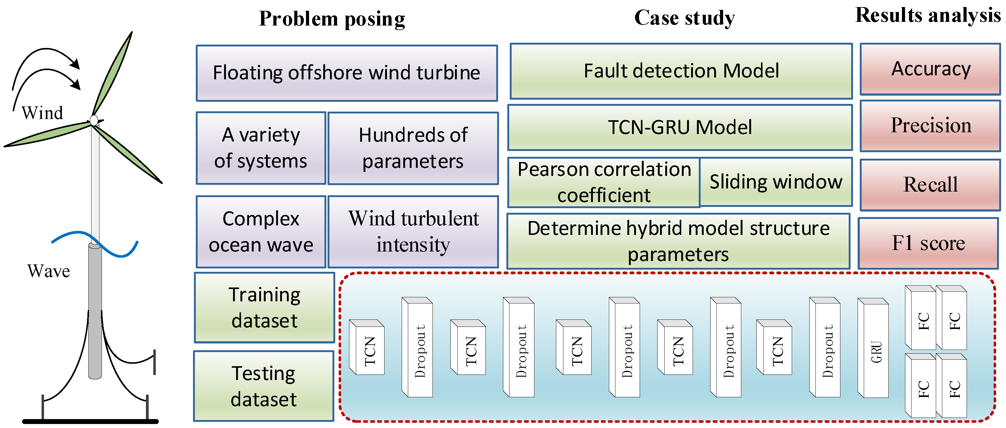
An integrated deep learning model based on TCN and GRU is proposed in this study for fault detection and detection in wind turbine drive systems. The drive system, consisting mainly of a gearbox and bearings, enables real-time monitoring of the system’s health status through the analysis of vibration acceleration signals. Random gradient descent is used as the optimization algorithm during the data training phase, and the network parameters are optimized through stochastic gradient descent. The detection results are output after the network training is completed. The proposed TCN-GRU model adopts a hierarchical feature extraction and sequence modeling combined architecture, as shown in Figure 2. The model is composed of four core components:

(1)

Input Preprocessing Module: The raw vibration signals are standardized and augmented by this module. The continuously collected acceleration signals are converted into a format suitable for processing by deep learning models. Consistent numerical ranges and statistical properties are ensured for signals collected under different operating conditions and from different sensors.

(2)

TCN Feature Extraction Module: This module consists of five TCN blocks and corresponding Dropout layers alternately stacked. Multi-scale temporal features are hierarchically extracted through progressively increasing dilation factors. Discriminative features related to faults in the vibration signals are automatically learned by this module, without requiring manual feature engineering.

(3)

GRU Sequence Modeling Module: The high-dimensional feature sequences extracted by the TCN are received by this module. Temporal dependencies and dynamic evolution of the features are modeled through gating mechanisms. The gradual process of fault development and transient features related to state transitions are captured by this module.

(4)

Fully Connected Classification Module: The sequence features encoded by the GRU are mapped to the fault category space by this deep classifier, which consists of four fully connected layers. Accurate classification of various operating conditions, such as normal states, gear faults, and bearing faults, is achieved by this module.

Feature extraction and fault classification of transmission system vibration signals are achieved by the TCN-GRU architecture through hierarchical time series and gated control units. In this framework, the raw data are first organized into batch form as ${\mathbf{X}}_{raw}\in {\mathbb{R}}^{B\times C_{in}\times T}$, where B represents the batch size, $C_{\mathrm{in}}$ represents the number of input channels (corresponding to the acceleration measurement channels of the main shaft, low-speed shaft, medium-speed shaft, and high-speed bearing), and T represents the time series length. Temporal features are subsequently captured by five TCN blocks through standard one-dimensional convolution. The number of feature channels is expanded from $C_{\mathrm{in}}$ to $C_{\mathrm{out}}$ while the temporal dimensions are preserved. The transformed output feature matrix ${\mathbf{H}}^{\left(L\right)}\in {\mathbb{R}}^{B\times C_{out}\times T}$ is reorganized and then input to the GRU layer. Global sequence modeling is performed through the gating mechanism.

The reorganized sequence data are received by the GRU layer. Each time step corresponded to a $C_{\mathrm{out}}$ dimensional feature vector. Historical information was selectively retained and updated through the gating mechanism of the update gate, reset gate, and candidate hidden state. The entire time series is compressed into an H dimensional hidden state representation $\mathrm{h}\in {\mathbb{R}}^{B\times H}$, where H is the GRU hidden state dimension. This compressed representation contained the global temporal patterns and fault feature information of the sequence. Finally, classification decisions are made through a two-layer fully connected network based on the hidden state output by the GRU. End-to-end fault detection is achieved.

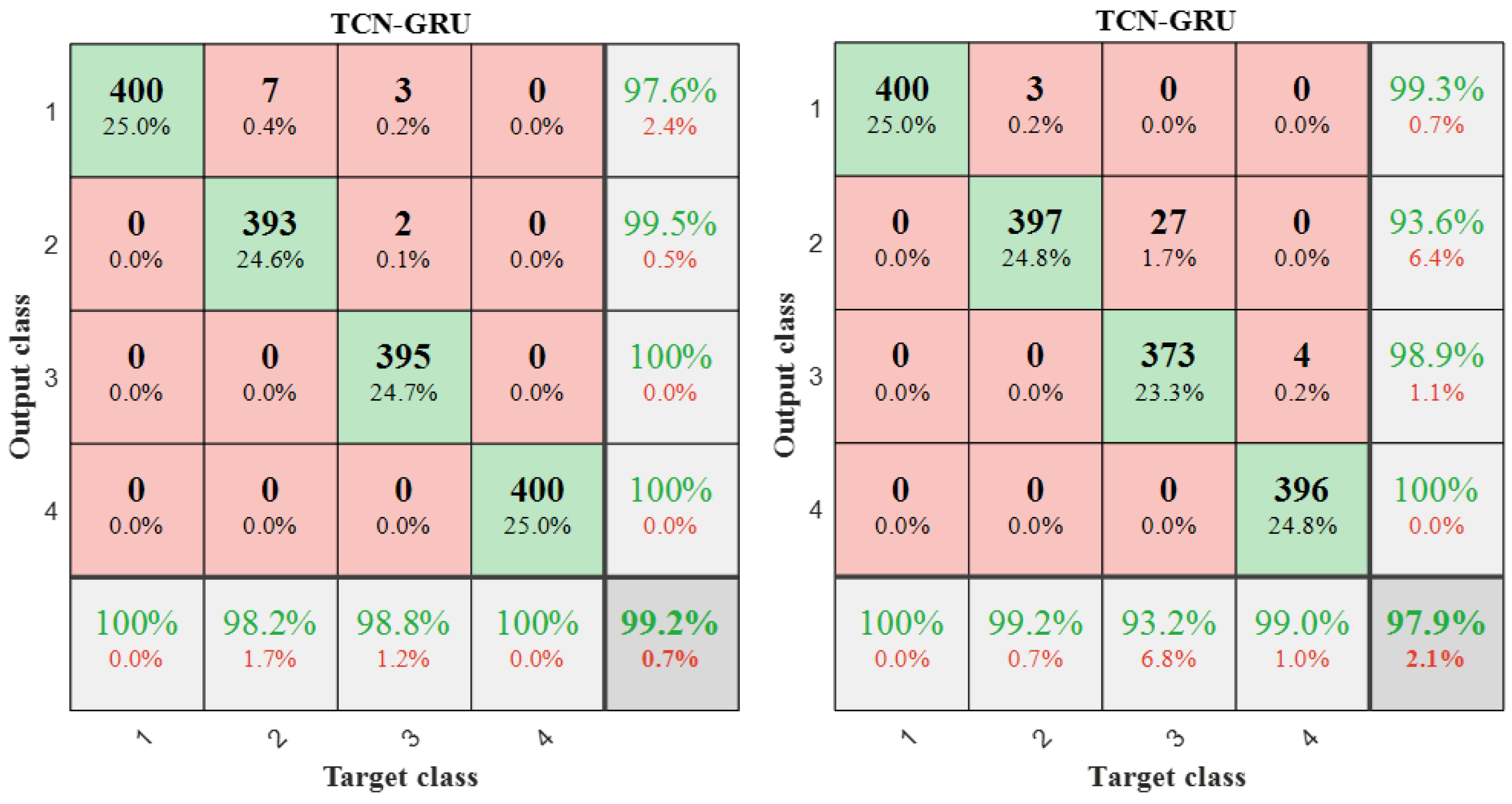
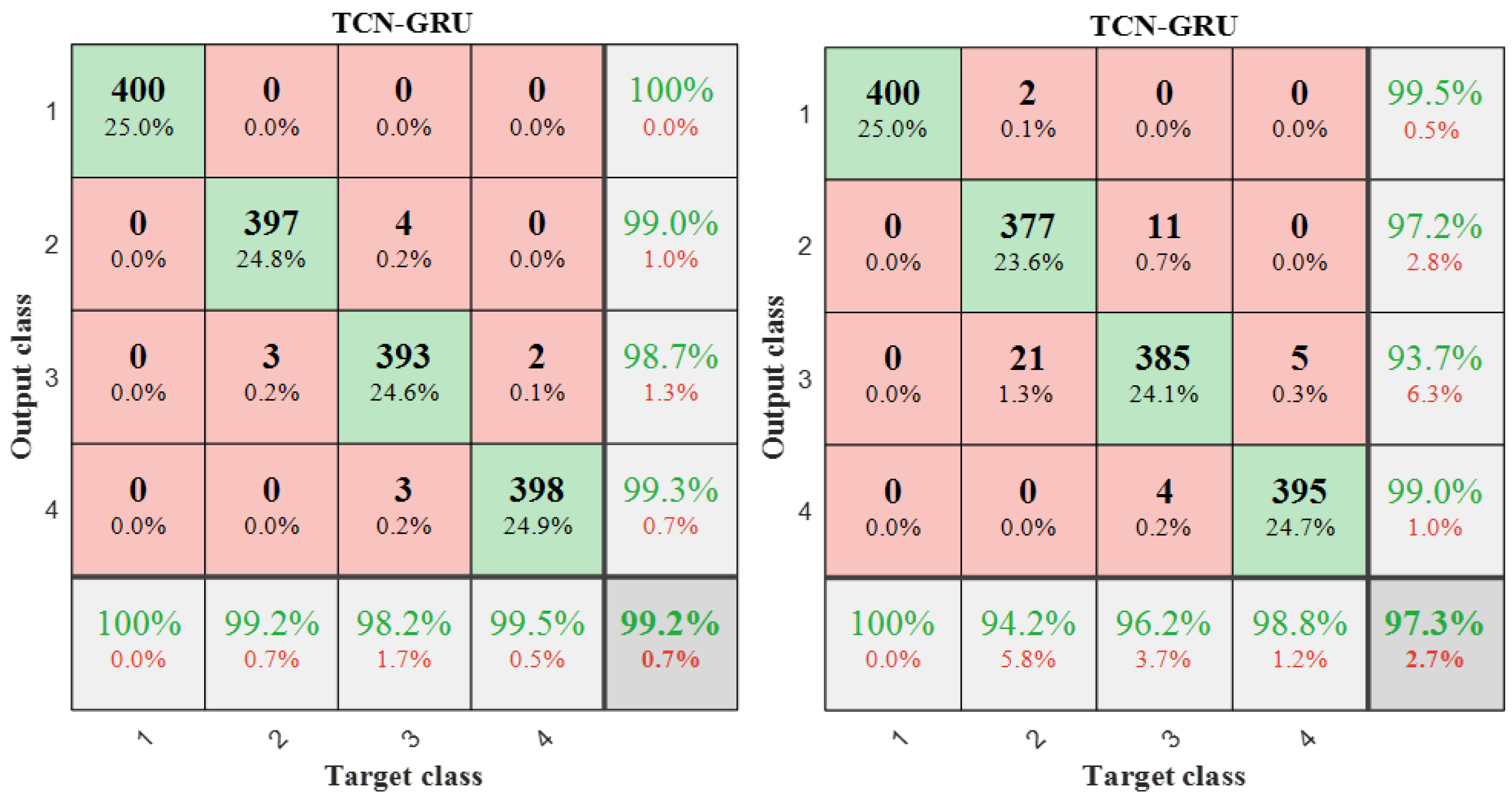
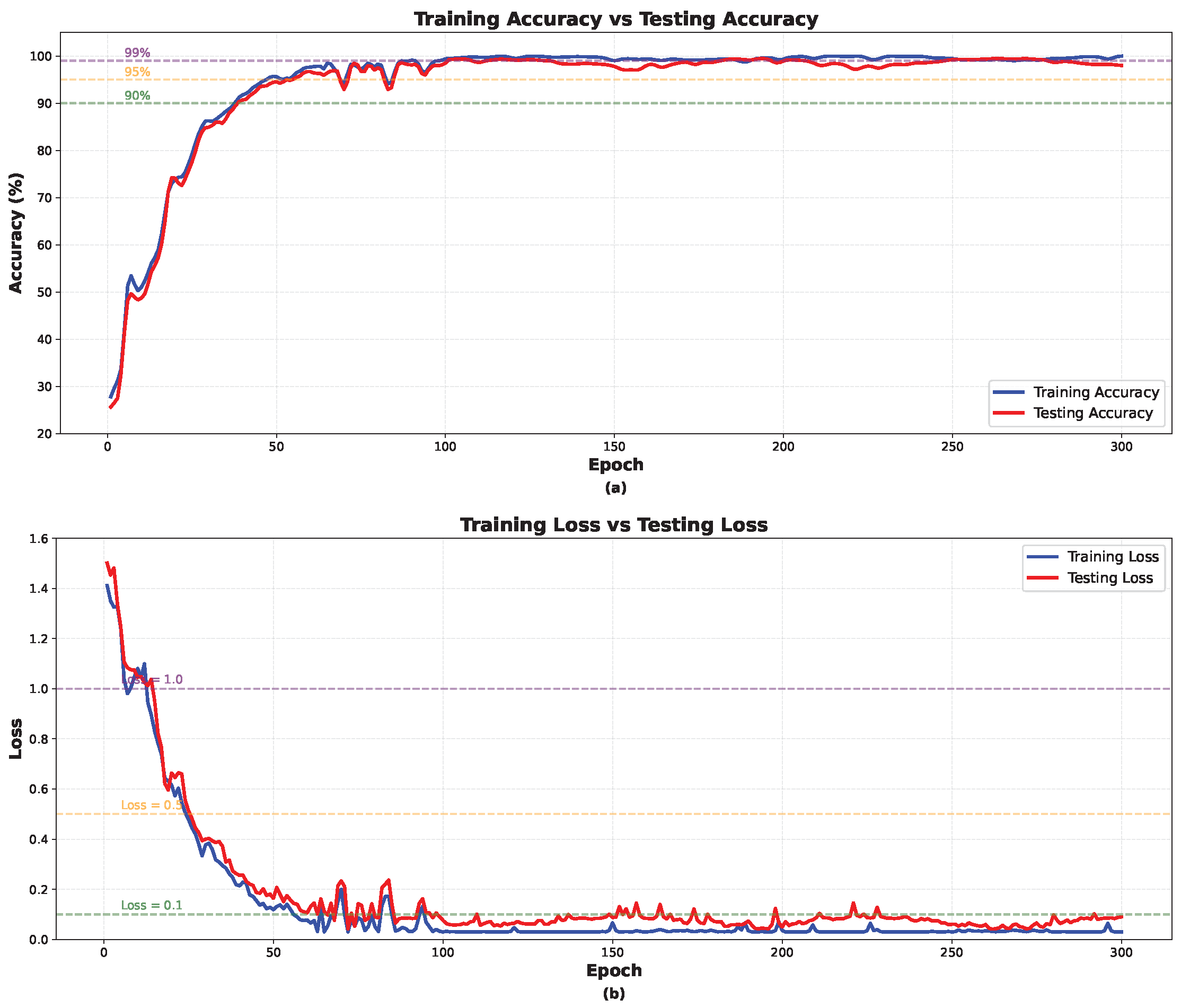
The entire TCN-GRU hybrid architecture realized an end-to-end mapping from 4-dimensional vibration features to 4 fault condition categories. The advantages of TCN in local feature extraction and the capability of GRU in sequence modeling are fully integrated. Accurate and reliable solutions for fault detection of transmission systems are provided. The discriminative ability of the model for different fault types can be comprehensively evaluated through confusion matrices and accuracy assessment.

3.4. Method Details

3.4.1. Detailed Introduction to the TCN Module

The TCN module is the core component of the model, with its design carefully considering the causal characteristics of time series data. The module is composed of five stacked TCN layers, with a dilated convolution strategy applied to gradually expand the receptive field, thus constructing a deep network structure with strong temporal modeling capability [34]. To satisfy the causality constraint required for temporal prediction, a causal convolution mechanism is employed in each TCN layer. 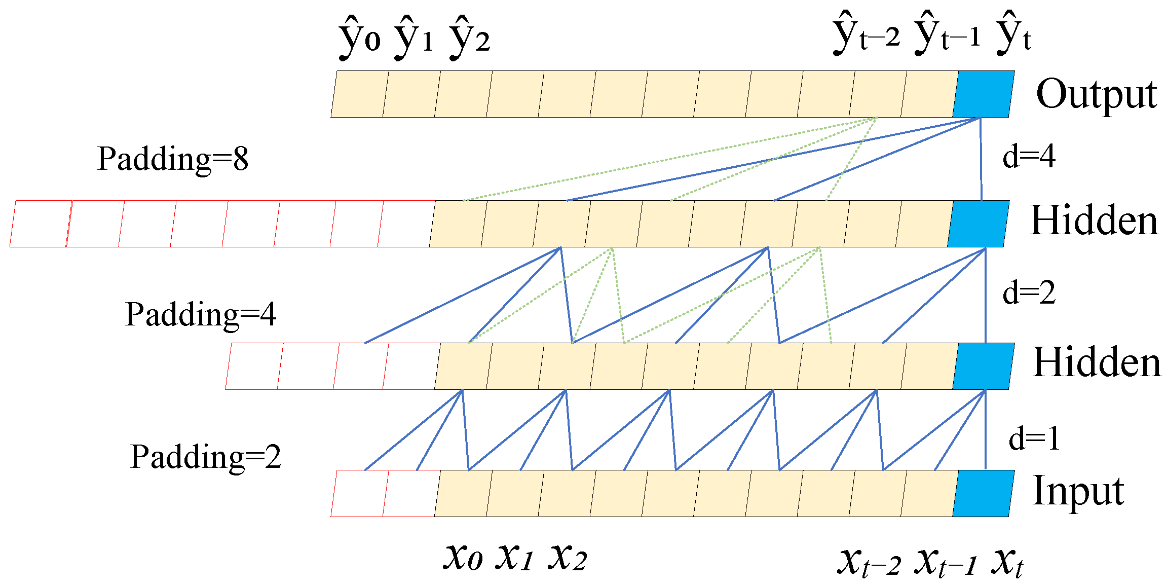It is ensured that the output at time t depends only on the inputs at time t and earlier, with the unidirectional flow of time being strictly followed. This causal design guarantees that no future information is used during prediction, preventing information leakage and allowing the model to accurately capture the temporal evolution of vibration signals. The specific structure of the causal convolution is shown in Figure 3.

Considering that the input data consists of 4-dimensional features, the TCN structure parameters have been carefully adjusted to accommodate this specific signal characteristic. The 4-dimensional input signals, which contain the key feature measurements of the system, are processed using standard 1D convolution operations by the TCN for feature extraction. The mathematical expression for the standard convolution operation is as follows:

$$\left(\mathbf{X}{\ast }_d\mathbf{F}\right)\left(t\right)=\sum _{c=1}^{C_{\mathrm{in}}}\sum _{i=0}^{k-1}\mathbf{F}(c,i)·{\mathbf{X}}_{c,t-d·i}$$

(2)

where, $C_{in}=4$ represents the number of input channels, which correspond to measurements from four axes in two directions. $\mathbf{F}\in {\mathbb{R}}^{C_{out}\times C_{in}\times k}$ is the learnable convolution filter. d is the dilation factor, controlling the spacing between sampled points. k is the filter size. The causality constraint $t-d·i\ge 0$ ensures that only historical and current information is used by the model, preventing future information leakage. This is crucial for real-time fault detection systems, as it guarantees the model’s feasibility during actual deployment.

As illustrated in Figure 4, Temporal Convolutional Networks with dilated convolutions can achieve an extensive receptive field even with a shallower network architecture. This allows for efficient temporal modeling while mitigating the vanishing gradient problem during training [35]. After introducing dilated convolutions, the receptive field can be expressed as:

$$R{F}_L=1+(k-1)·\sum _{\mathrm{i}=0}^{L-1}{\mathrm{d}}_{\mathrm{i}}$$

(3)

where, $d_i$ is the dilation factor of the $\mathit{i}\text{-}\mathit{th}$ layer of causal convolution, typically set to $d_i=b^i$, and b is referred to as the base dilation factor.

Temporal dependencies are ensured by TCN through causal convolution. During the feature propagation process, long-range dependencies in the input data are captured by extracting important features over extended time periods. Data with long sequence lengths and complex features can be effectively handled by TCN. Additionally, strong parallel computing capabilities and more stable gradient propagation are offered by TCN layers. These advantages are particularly demonstrated when processing long sequences [36].

3.4.2. Detailed Introduction to the GRU Module

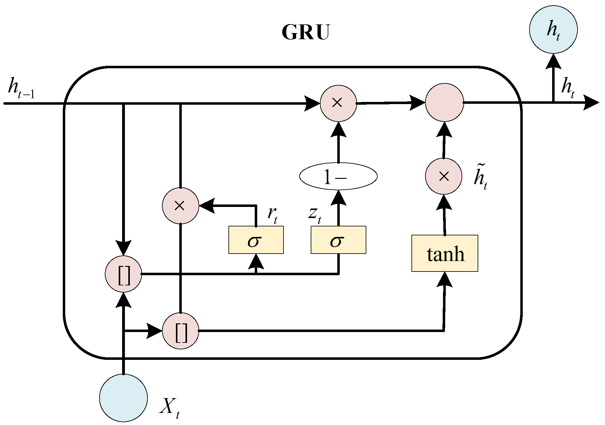
The GRU serves as the core sequence modeling component of the model. It is responsible for converting the spatial features extracted by TCN into temporal representations. In the fault detection of wind turbine transmission systems, vibration signals contain not only transient impact characteristics but also the dynamic evolution process of fault development. Therefore, a GRU layer is introduced after TCN feature extraction to perform further sequence encoding on the extracted features.The architecture of the GRU model is illustrated in Figure 5. The number of parameters is reduced by this structure, while performance comparable to LSTM is still maintained in many scenarios. Such design makes GRU highly efficient in processing sequential data, particularly when a lighter model or faster training is required [37].

The high-dimensional feature sequence from TCN is received by GRU. First, dimension reorganization needs to be performed to accommodate the requirements of recurrent processing. The feature tensor output by TCN undergoes dimension permutation to be converted into a temporal format:

$$s=\mathrm{Permute}\left({\mathbf{H}}^{\left(5\right)}\right):{\mathbb{R}}^{B\times 64\times N}\to {\mathbb{R}}^{B\times N\times 64}$$

(4)

where, ${\mathbf{H}}^{\left(5\right)}$ represents the feature tensor output from the 5th layer of TCN. B denotes the batch size, 64 represents the number of channels, and N indicates the sequence length. S is the reorganized sequential feature. Each time step corresponds to a 64-dimensional feature vector. The Permute operation exchanges the channel and time dimensions. Each time step t is enabled by this transformation to correspond to a set of vibration characteristics encompassing all scales at that moment.Through the stacking of 5 standard convolution layers, the feature vector at each time step integrates temporal patterns from local to medium scales. The theoretical receptive field spans 11 time steps. This is sufficient to capture critical changes in vibration characteristics.

The update gate, reset gate, and candidate hidden state together form the core computational mechanism of the GRU. The mathematical expression for this mechanism is as follows:

$${\mathbf{z}}_t=\sigma ({\mathbf{W}}_z{\mathbf{s}}_t+{\mathbf{U}}_z{\mathbf{h}}_{t-1}+{\mathbf{b}}_z)$$

(5)

$${\mathbf{r}}_t=\sigma ({\mathbf{W}}_r{\mathbf{s}}_t+{\mathbf{U}}_r{\mathbf{h}}_{t-1}+{\mathbf{b}}_r)$$

(6)

$${\tilde{\mathbf{h}}}_t=\tanh ({\mathbf{W}}_h{\mathbf{s}}_t+{\mathbf{U}}_h({\mathbf{r}}_t\odot {\mathbf{h}}_{t-1})+{\mathbf{b}}_h)$$

(7)

where, ${\mathbf{W}}_z$, ${\mathbf{W}}_r$ and ${\mathbf{W}}_h$ are the weight matrices input to each gate, respectively. The features extracted by TCN are compressed into the gate control signal space. ${\mathbf{U}}_z$, ${\mathbf{U}}_r$ and ${\mathbf{U}}_h$ are the corresponding cyclic weight matrices. The self-feedback of the hidden state is captured. ${\mathbf{b}}_z$, ${\mathbf{b}}_r$ and ${\mathbf{b}}_h$ are the bias vectors. ⊙ represents the Hadamard product (element-wise multiplication).

In the processing of wind turbine vibration signals, unique adaptability is exhibited by this mechanism. The update gate determines the proportion of historical information to be retained and new information to be accepted at each time step. The sigmoid activation function limits the gate value within the range of [0, 1], which corresponds physically to the proportion of information that is passed. Selective forgetting is achieved by the reset gate, with the extent of historical information usage being controlled to precisely manage memory. The current input is combined with the history filtered by the reset gate to generate a new estimate for the current state by the candidate hidden state.

3.4.3. Fully Connected Network Classification

The fully connected network serves as the final decision-making module of the TCN-GRU architecture. The time-series features encoded by GRU are mapped to the fault category space. The multi-class fault detection is calculated based on the following formulas:

$${\mathbf{z}}_{fc1}={\mathbf{W}}_{fc1}·{\mathbf{h}}_{avg}+{\mathbf{b}}_{fc1}$$

(8)

$${\mathbf{z}}_{fc2}={\mathbf{W}}_{fc2}·{\mathbf{f}}_1^{drop}+{\mathbf{b}}_{fc2}$$

(9)

where, ${\mathbf{W}}_{fc1}$ is the weight matrix of the first fully connected layer. The time-series features output by GRU are mapped to a higher-dimensional feature space by this matrix. ${\mathbf{W}}_{fc2}$ is the weight matrix of the second fully connected layer. The 64-dimensional features are mapped to 4 fault categories by this matrix. ${\mathbf{b}}_{fc1}$ and ${\mathbf{b}}_{fc2}$ are the bias vectors of the corresponding layers, respectively. ${\mathbf{h}}_{avg}$ is the average value of the time-series features output by GRU. ${\mathbf{f}}_1^{drop}$ is the output after the first fully connected layer passes through ReLU activation and Dropout processing.

Discriminative mapping from multi-dimensional time-series features to specific fault categories is achieved by the classification module through progressive feature transformation. The dimensionality of feature representation is increased by the first fully connected layer. The network is enabled to learn more complex decision boundaries. The weight matrix ${\mathbf{W}}_{fc1}$ is learned through training to map from time-series features to high-dimensional discriminative space optimally. Non-linear activation is introduced by the ReLU activation function. The similarity between fault categories is captured. Overfitting is prevented by the Dropout mechanism applied simultaneously. The dimensionality is gradually reduced in subsequent fully connected layers. A golden pyramid structure of features is formed. The probability distribution of fault categories is finally obtained through the Softmax function. Accurate identification of normal state, gear fault, bearing fault, and other working conditions is achieved.

4. Results and Analysis

4.1. Model Evaluation Metrics

To validate the effectiveness of the TCN-GRU model in bearing fault detection for offshore wind turbines, four evaluation metrics were adopted: accuracy, precision, recall, and F1-score. These metrics were used to assess the performance of the deep learning architecture employed in this study. The formulas for the four evaluation metrics are as follows:

$$\mathrm{Accuracy}={\displaystyle \frac{TP+TN}{TP+TN+FP+FN}}$$

(10)

$$\mathrm{Precision}={\displaystyle \frac{TP}{TP+FP}}$$

(11)

$$\mathrm{Recall}={\displaystyle \frac{TP}{TP+FN}}$$

(12)

$$\mathrm{F}1={\displaystyle \frac{2·\mathrm{Precision}·\mathrm{Recall}}{\mathrm{Precision}+\mathrm{Recall}}}$$

(13)

where, accuracy represents the proportion of all samples that are correctly classified by the model, TP represents the number of faults correctly identified by the model, TN represents the number of non-faults correctly identified by the model, FP represents the number of non-faults incorrectly identified as faults by the model, and FN represents the number of actual faults that the model failed to identify. Precision indicates how many of the samples identified as faults by the model are indeed true faults. Recall measures how many actual fault cases are correctly identified by the model. The F1-score is the harmonic mean of precision and recall, serving as a comprehensive evaluation metric. A high F1-score indicates a more harmonious balance between the diagnostic model precision and recall, which suggests that the model has achieved an optimal performance level.

4.2. Hyperparameter Settings

The proposed TCN-GRU model was implemented using MATLAB R2021a (MathWorks, Natick, MA, USA) with the Deep Learning Toolbox. The network was trained on an NVIDIA GPU with the hyperparameters listed in

Table 5. Hyperparameter settings.

Hyperparameter	Value
Epochs	300
Batch size	96
Optimizer	SGDM
Initial learning rate	0.005
Learning rate schedule	Piecewise
Learning rate drop factor	0.5
Learning rate drop period	40 epochs

. The setting of hyperparameters for neural networks is crucial. The random gradient descent method is used for optimization, where the algorithm randomly selects samples to compute gradients and update model parameters, thus reducing the computational cost. The escape from local minima is facilitated by the inherent randomness of this method. Convergence to the global minimum is made easier, and the model generalization ability is enhanced. As a result, greater adaptability to the dataset is achieved by the model. In the experiment, the number of training epochs is set to 300, with an initial network learning rate of 0.005. The learning rate decay factor is 0.5, and the learning rate is decreased every 40 epochs. The number of hidden units corresponds to the size of the hidden state vector in each batch. A large number of hidden units reflects an increase in model complexity, but for a given system and data attributes, networks with too many hidden units may cause data overfitting. Additionally, errors can be excessive when the batch size is too large or too small. After multiple tests, the batch size is set to 96 in this experiment. The L2 regularization coefficient is used by adding a penalty term in the loss function to constrain the size of the model parameters, thus preventing overfitting. The form of L2 regularization is the sum of the squares of all model weights, multiplied by a penalty coefficient. Through the penalization of excessively large weights, a simpler model is encouraged by L2 regularization, which prevents overfitting on the training data. The L2 regularization coefficient is set to 0.0008.

4.3. Experimental Results and Analysis

4.3.1. Correlation Coefficient Analysis Results

In the overall analysis of the Pearson correlation coefficient heatmap, strong inter-feature correlations were observed in the axial data, whereas the radial data showed a tendency for weaker inter-feature correlations. The features shown in Figure 6 correspond to the main shaft, low-speed shaft, intermediate-speed shaft, and high-speed shaft, respectively. In the EC1-A condition, the main shaft and low-speed shaft consistently demonstrated high correlation across all three subplots, with a correlation coefficient of 0.9785. This indicates a strong linear relationship between these two features. In EC3-A, the correlation between the main shaft and intermediate-speed shaft was relatively weaker yet still showed a certain degree of association, with a correlation coefficient of 0.2624, which reflects a moderately weak positive correlation. The correlation between the low-speed shaft and intermediate-speed shaft was also notable, with a correlation coefficient of 0.3645. This suggests a fairly strong relationship between these two features.

In contrast, the features within the radial data exhibit significantly weaker correlations among themselves. The correlation coefficients between features are generally low, approaching zero, which indicates negligible linear relationships between them. For instance, in EC2-R, the correlation coefficient between Feature 1 and Feature 3 is 0.0089, which suggests an almost nonexistent linear relationship. Correlations among other features are also very weak—for example, the correlation between Feature 1 and Feature 4 is 0.0035, further supporting the independence among these features.

Based on the analysis of these correlation coefficients, it can be concluded that the axial data demonstrate strong positive correlations, which reflect a high degree of interdependence among the features in the axial direction. In contrast, features in the radial data generally show weak correlations, which indicates that they are relatively independent. Therefore, subsequent research should verify whether the high correlation observed in the axial data leads to higher accuracy rates.

4.3.2. Fault Detection Results

A deep learning model based on TCN-GRU was developed to identify the health state and three different fault conditions of wind turbine blades. The model was evaluated under three distinct environmental conditions—below-rated, rated, and above-rated wind speed—where its fault detection performance was assessed. Multiple performance metrics, including accuracy, precision, recall, and F1-score, were employed to comprehensively evaluate the model effectiveness. A confusion matrix was plotted to visually represent the classification outcomes. The dataset was partitioned into 80% for training and 20% for testing.

A comparative experiment was conducted to evaluate the classification performance of five neural network architectures: CNN, CNN-LSTM, CNN-GRU, TCN, and TCN-GRU. As shown in Figure 7, Figure 8 and Figure 9, the best performance across all wind speed conditions was achieved by the TCN-GRU model. Under below-rated wind speed, an accuracy of 0.943 was attained by TCN-GRU, outperforming both TCN and CNN-GRU. At rated wind speed, the accuracy of all models decreased, with TCN-GRU still maintaining the highest accuracy of 0.886, while CNN-LSTM achieved only 0.854. It was observed that wind speed conditions had a notable influence on model performance. Specifically, near the rated wind speed, the detection accuracy of all models declined. This phenomenon is likely attributed to the fact that wind turbines operate under rated power control in this region, where fluctuations in aerodynamic loads interfere with fault-related features. Consequently, stronger feature extraction capabilities are required by models under high turbulence or near-rated wind conditions. In comparison, the temporal dependency modeling ability of TCN and the sequential learning capacity of GRU are combined in TCN-GRU, which leads to more stable fault recognition under varying wind speeds. This result indicates that the proposed model is not only suitable for steady conditions but also exhibits strong adaptability in dynamic environments.

In the EC1 condition, high accuracy in identifying the healthy state was demonstrated, with a correct classification rate of 97.6% achieved. For Fault Type 1, a precision of 100% was yielded, with no false alarms during prediction. The recall rates for Fault Type 2 and Fault Type 3 were 98.2% and 100%, respectively, suggesting that most faulty samples were successfully detected. However, a slightly higher missed detection rate was observed for Fault Type 2. The F1-score was reached at 98.8%, reflecting a well-balanced performance across different fault categories. Compared to existing fault detection methods, superior accuracy was exhibited across all tested environmental conditions, with an overall accuracy of 99.2%. This result significantly outperformed the 95% accuracy achieved by conventional methods under similar operational conditions, demonstrating that stronger adaptability in handling complex temporal data is possessed by the TCN-GRU model.

As shown in Figure 10, Figure 11 and Figure 12 under three different environmental conditions, the model based on axial data demonstrates relatively stable performance and achieves the highest accuracy rates of 99.2%, 99.1%, and 99 %, respectively. These results indicate that highly consistent classification performance is maintained by the model across varying wind speeds and turbulence intensities, with particularly low misclassification rates observed in fault detection. The high accuracy is reflected by the sensitivity of axial data to the fault conditions of the wind turbine, which allows for the detection of subtle variations and enhancement of the model diagnostic capability. In contrast, the model based on radial data shows fluctuating performance under the three environmental conditions, with accuracy values of 97.9%, 94.6%, and 97.3%, respectively.Notably, under the second environmental condition—characterized by higher wind speed or stronger turbulence—the classification accuracy of radial data decreases to 94.6%, indicating certain challenges to the model robustness in such scenarios. This decline may be attributed to the insensitivity of radial data to certain fault types or increased susceptibility to noise under high-turbulence conditions. By comparing the classification results between axial and radial data, it is evident that axial data generally yields higher accuracy. Particularly in complex environments, radial data are more prone to disturbances, whereas axial data exhibit superior stability. The stronger perceptiveness of axial data to state changes in wind turbines underscores its critical role in both model training and fault detection processes.

The proposed TCN-GRU model demonstrates excellent performance over 300 training epochs. As shown in Figure 13, both the training accuracy (blue curve) and the testing accuracy (red curve) increase steadily, ultimately reaching a high level. In the early training stage, the model exhibits pronounced rapid-learning behavior: the accuracy rises from about 27% to about 90%, indicating a strong ability to quickly capture drivetrain fault signatures. The model also shows good generalization, with the training and testing accuracies remaining closely aligned and a generalization gap of only 2–3%, suggesting no evident overfitting. This rapid learning indicates that the adopted network architecture and feature-extraction strategy effectively identify fault patterns in drivetrain vibration signals. During the final 200 epochs, the model maintains highly stable performance without the large late-stage oscillations in accuracy often associated with training instability.

5. Conclusions

This study proposes an integrated TCN-GRU deep learning model to address fault detection challenges in floating offshore wind turbine drivetrains under complex marine conditions. By combining TCN’s multi-scale temporal feature extraction with GRU’s capability to capture long-term degradation patterns, the proposed model demonstrates superior performance compared to Traditional deep learning models across multiple operational conditions. The integration of temporal and recurrent mechanisms proves particularly effective in handling the dynamic coupling effects between platform motions and drivetrain vibrations, which are characteristic of floating offshore installations. While this study establishes a robust framework using validated simulation data, future work will focus on applying the model to field monitoring data to verify its performance under actual operating conditions with sensor noise, environmental uncertainties, and real degradation mechanisms. This research provides a foundation for developing practical condition monitoring systems for offshore wind turbine drivetrains.