Abstract
Highways constructed on stratified foundations with thick soft soil interlayers in the Yellow River floodplain of Shandong Province have experienced long-term settlement. However, accurately predicting subgrade settlement caused by the secondary consolidation of soft soils remains a major engineering challenge. In this study, PLAXIS 3D numerical simulation was combined with a neural network model to predict the long-term temporal and spatial settlement behavior of highway subgrades. The results show that the soft soil creep (SSC) constitutive model better represents the consolidation process of the soft soil interlayer than the soft soil (SS) model. A decrease in permeability will prolong the dissipation time of excess pore water pressure and the settlement stabilization time, leading to an increase in the proportion of post-construction settlement in the total settlement. The final settlement increases linearly with the thickness of the soft soil interlayer and embankment height, while it decreases following a power-law function with increasing interlayer burial depth. By comprehensively considering the combined effects of multiple factors, a genetic algorithm–optimized backpropagation neural network (GA-BP) model was developed. The testing dataset achieved a root mean square error (RMSE) of 0.01488 m, a mean absolute percentage error (MAPE) of 7.0562%, and a coefficient of determination (R2) of 0.9706, demonstrating the model’s ability to achieve intelligent full-period and full-section settlement prediction for subgrades with soft soil interlayers. Overall, this study developed an intelligent framework for predicting long-term settlement in subgrades with soft soil interlayers, offering practical guidance for evaluation and timely settlement control.
1. Introduction
The Yellow River floodplain in Shandong Province is characterized by widely distributed layered foundations and the presence of thick soft soil interlayers, which pose significant safety risks for the long-term operation of highways. Currently, post-construction settlement prediction and control of existing subgrades is a critical technical issues during highway operation. With the continuous refinement of advanced soil mechanics theories [1], various methods for calculating the settlement of existing subgrades have been developed. Common methods include the layer summation method [2], data extrapolation methods [3], and numerical simulation [4]. However, the layer summation method does not account for the lateral displacement of the soil structure, resulting in considerable computational errors. Based on field-measured data, fitting methods such as the hyperbolic method [5], exponential curve method, and Asaoka methods [6] have been proposed, but these require long-term observation and are significantly influenced by the accuracy of the monitoring data. The finite element method (FEM) numerical simulation can more comprehensively consider characteristics such as soil constitutive behavior, consolidation effects, porous structure, Young’s modulus and permeability, offering higher feasibility, applicability, and accuracy in predicting the settlement of subgrades and other structures [7,8,9,10].
Moreover, different methodologies have been developed and presented by researchers to enhance the predictive performance and field applicability of these models. Hsieh et al. [11] introduced a technique that effectively forecasts ground surface settlement and angular distortion for concave and spandrel settlement profiles. Li et al. [12] employed a time-series model to estimate total settlement during roadbed filling operations. Li et al. [13] developed a hybrid approach that integrates an exponential curve with artificial neural networks (ANN) to categorize roadbed settlements into certain and uncertain components. To further improve prediction accuracy, various innovative approaches have been explored. Hui et al. [14] presented the twin support vector regression method, which outperformed traditional support vector regression in forecasting accuracy. Huang et al. [15] introduced a Richards model based on the bidirectional difference-weighted least-squares (BD-WLS) technique, enhancing the accuracy of soft soil subgrade settlement predictions. By combining a limited amount of actual settlement data obtained from intelligent monitoring equipment with regression analysis and machine learning techniques, settlement prediction can also be effectively achieved [16,17,18,19].
Influenced by the Yellow River floodplain, there is a certain thickness (ranging from 1 to 4 m) of soft soil interlayer in the foundation of the Shandong section of the highway. Even after several years of operation, the highway continues to experience settlement. According to on-site monitoring data, during the 15 years since the highway opened to traffic, uneven settlement has occurred in multiple sections of the subgrade. In areas where the soft soil interlayer is approximately 4 m thick, the maximum settlement has reached 38 cm, significantly exceeding highway subgrade design and construction standards. Accurate and timely prediction of time-dependent deformation behavior in soft soils is essential, as it significantly mitigates threats to infrastructure resilience. By furnishing accurate predictions, stakeholders can implement proactive mitigation strategies, optimize design and construction methodologies, and minimize the likelihood of unforeseen losses and damage.
This study, centered on a prototype highway in Shandong, employs creep parameters to ascertain the time-dependent settlement characteristics of the existing subgrade. Using PLAXIS 3D finite element software (PLAXIS 3D CE V20), the model simulates the consolidation characteristics of layered foundation soils. The finite element constitutive model of the soft soil interlayer is based on the Soft Soil Creep (SSC) model to calculate post-construction subgrade settlement on soft soil foundations. By comparing the numerical results with field-measured data, the rationality and reliability of the finite element model were validated. Numerical simulations were performed to analyze subgrade settlement over the service life, considering different geotechnical properties of the soft soil. The analysis examined the effects of consolidation time, soft soil interlayer permeability, soft soil interlayer thickness, burial depth, and subgrade height on settlement. Furthermore, this study proposes a settlement prediction method for soft soil interlayer foundations in the Yellow River floodplain region, using deep learning neural networks with multi-parameter inputs.
2. Soil Constitutive Model and Parameter Determination
Both the Soft Soil Model (SS) and the Soft Soil Creep Model (SSC) are second-order models based on the viscoplastic theory framework included in PLAXIS software [20]. They are used to simulate time-dependent characteristics of normally consolidated clays and peat, among other soft soils. The SS model, built on the Mohr–Coulomb criterion, incorporates a broader range of soil behavior characteristics, providing a more accurate description of the nonlinear behavior of soft soil foundations under compression and shear [21]. As an extension of the SS model, the SSC model introduces the concept of secondary compression in soft soils, integrating primary and secondary consolidation of the soil mass to better reflect the volumetric creep characteristics of soft soil. In the SSC constitutive model, the total volumetric strain is defined as:
Here, represents the total volumetric strain generated when the average effective stress increases from to over a certain period. denotes the elastic volumetric strain, and denotes the viscoplastic volumetric strain, which is further divided into primary consolidation strain () and secondary consolidation strain (). represents the time at which primary consolidation is complete, is the time for secondary consolidation and effective creep, is the initial effective stress before embankment construction, is the final load effective stress, and are the pre-consolidation pressure and final consolidation pressure before embankment construction, respectively. is the corrected swelling index, is the corrected compression index, and is the corrected creep coefficient. The SS constitutive model is formulated by removing the secondary consolidation portion from the viscoplastic volumetric strain in the SSC model.
3. Computational Model and Soil Parameters
Numerical calculations are conducted using the PLAXIS 3D hydro-mechanical consolidation finite element program, employing tetrahedral mesh elements with pore water pressure monitoring defined at the center of each element.
3.1. Subgrade Model
Based on site-specific geological investigation data, the ZK111 profile of the highway subgrade section is highlighted in Figure 1. The analysis in this study is based on the section exhibiting the highest measured settlement.
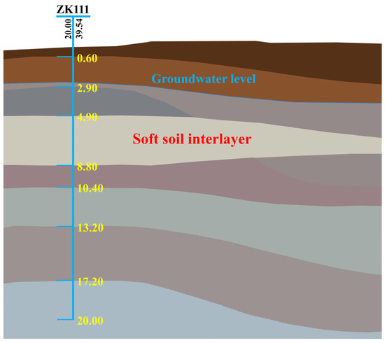
Figure 1.
Calculation of cross-section geologic profiles (unit: m).
For a section of the subgrade with a 4-m-thick soft soil interlayer, a three-dimensional finite element analysis model of the subgrade and foundation was established, as shown in Figure 2, based on the actual highway width. To simplify the modeling and analysis process, the model represents half of the highway subgrade, with a thickness of 2.0 m and a total height of 28.0 m. This includes a foundation soil thickness of 20.0 m and an embankment height of 8.0 m. The horizontal length of the foundation is set to 60.0 m to mitigate the effects of boundary conditions, while the width of the road surface is 14.0 m, with a slope gradient of 1:1.5. The groundwater level is set at 2.5 m below the foundation. During the calculations, the lateral boundaries of the finite element model are constrained in the normal direction, and the bottom boundary is fully fixed. Considering the transverse symmetry and longitudinal continuity of the subgrade, the Boundary X-Min, Boundary Y-Min, and Boundary Y-Max in the groundwater seepage conditions are set as undrained. In contrast, to account for the hydraulic connectivity of groundwater during the long-term settlement process, the Boundary X-Max, Boundary Z-Min, and Boundary Z-Max are set as drained. Initial pore pressures in the soil layers are set to hydrostatic pressure. The dimensions of the subgrade and soil distribution are illustrated in Figure 2. The subgrade construction period is 100 days, after which the settlement development over time is calculated in conjunction with the consolidation settlement process.
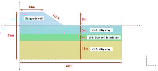
Figure 2.
Finite element model of the subgrade.
To improve computational efficiency, the following simplifications were applied to the soil parameters:
- The multi-layer embankment loading model is simplified to a single-layer embankment loading, with the embankment load applied over a period of 100 days, ignoring the stabilization period between the compaction of successive fill layers.
- Multiple soil layers below the soft soil interlayer are treated as a single layer of silty clay. The subgrade is divided into C-1, S-1, and C-2 layers, with the upper layer being floodplain silty clay, the middle layer being silty soft soil interlayer, and the lower layer being silty clay.
- The constitutive model for the embankment soil and the two layers of silty clay employs the Mohr–Coulomb model. The constitutive model for the soft soil interlayer uses either the Soft Soil Creep (SSC) model or the Soft Soil (SS) model. Specific parameters such as soil unit weight, cohesion, and angle of internal friction are based on the geotechnical investigation report.
3.2. Analysis and Calculation of Soil Parameters
Based on triaxial tests and other laboratory experiments, the basic geotechnical parameters of undisturbed soil in each foundation layer were determined, as shown in Table 1. The schematic diagram of the experimental setup is shown in Figure 3. The Poisson’s ratio for all soil layers in the model is uniformly set to 0.3 based on empirical values. The typical range for Poisson’s ratio is as follows: for silt, 0.25–0.35; for silty clay, 0.35–0.45; and for clay, 0.40–0.50 [22]. The numerical differences are minor, and the lateral deformation of the soil has a negligible impact on the settlement of the foundation and subgrade.

Table 1.
Basic properties of soil.
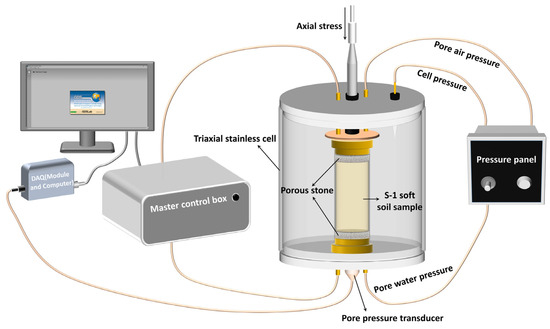
Figure 3.
Diagram of the triaxial apparatus experimental setup.
For undisturbed soil and remolded soil, the rebound index (), compression index (), and secondary consolidation coefficient () of the S-1 soil properties are essentially consistent and can be directly calculated based on consolidation tests. The modified swelling index (), modified compression index (), and modified creep coefficient () for the S-1 soft soil interlayer were calculated based on Equations (5)–(7) [23].
The relevant parameters for the Soft Soil (SS) and Soft Soil Creep (SSC) models are listed in Table 2.
Table 2.
Parameters related to S-1 soft soil interlayer constitutive modeling.
Seepage of groundwater within foundation soils can affect the stress distribution in the soil, leading to settlement [24,25]. Accurate prediction of settlement behavior in engineering practice requires comprehensive consideration of the permeability coefficient. This enables fluid–structure interaction analysis, which investigates both pore water pressure distribution and soil compressibility. The permeability coefficients of the foundation soils are presented in Table 3.
Table 3.
Soil permeability coefficient.
3.3. Correlation Analysis Between the Calculation Results and the Finite Element Mesh Size
To evaluate the influence of finite element mesh size on the computational results and ensure convergence, a systematic mesh sensitivity analysis was conducted in PLAXIS. The relative element size factor (re) in the software was adopted as the key parameter to control mesh density. Five different levels of re were selected, ranging from very coarse (re = 2.0) to very fine (re = 0.5), covering a broad range of mesh densities. For each re level, the corresponding average element size, total number of elements, and total number of nodes were calculated, as summarized in Table 4. The settlement–time curves at the subgrade centerline for different mesh sizes are presented in Figure 4. When re is smaller than 1.0, the settlement curves at different mesh levels tend to overlap, indicating that mesh size has little effect on the computational results. Therefore, to balance computational accuracy and efficiency, a fine mesh with re = 0.7 was adopted for all subsequent analyses.
Table 4.
Finite element mesh division parameter levels.
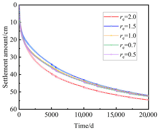
Figure 4.
Settlement at the subgrade centerline under different mesh density levels.
4. Settlement Prediction Calculation Result Analysis
4.1. Settlement in the Center of the Subgrade
Figure 5 presents the simulated variation in the settlement against time at the center of the subgrade under the SSC constitutive model for the soft soil interlayer. The red solid line represents linear time; the blue solid line represents logarithmic time. As shown in the figure, during highway construction, the settlement at the subgrade center increases rapidly, resulting in significant immediate settlement, reaching 8.81 cm by the end of construction. The settlement recorded after the post-construction increases remarkably during the initial 10,000 days, while the change in settlement is almost minimal as the consolidation period reaches 50,000 days. The final total settlement at the subgrade centerline is 61.90 cm, with post-construction settlement of 53.09 cm. Finite element analysis predicts that significant settlement potential remains in the subgrade, with stabilization taking an extended period.
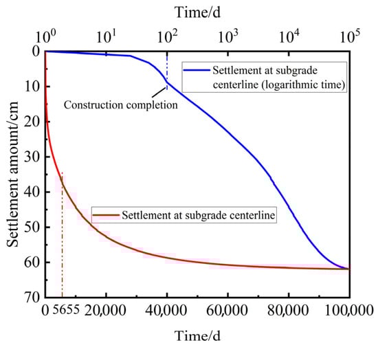
Figure 5.
Settlement characteristics observed at the center of the subgrade.
At the subgrade centerline of section ZK111, six on-site settlement measurements were conducted using the DSZ3 level instrument manufactured by South Surveying & Mapping at 800, 1650, 2600, 3680, 4400, and 5655 days, respectively. Figure 6 presents a comparison between the monitored and simulated settlements at the subgrade centerline of ZK111. In addition, the Root Mean Square Error (RMSE) and Mean Absolute Percentage Error (MAPE) were calculated using Equations (8) and (9) to evaluate the reliability and engineering applicability of the finite element model.
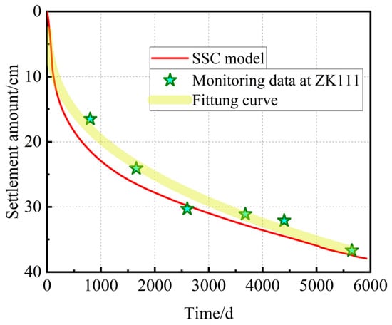
Figure 6.
Comparison between monitored settlement and simulated settlement at the subgrade centerline of ZK111.
In the formula, represents the monitored settlement value at time t; represents the simulated settlement value at time t; n is the number of samples in the dataset.
The calculated RMSE between the monitored and simulated settlement data is 2.5524 cm, accounting for 8.3965% of the average simulated settlement, which is less than 10%. The MAPE is 9.3510%, also below 10%. Therefore, there is a strong correlation and a small deviation between the simulated and monitored settlement values.
4.2. Analysis of the Impact of Soil Constitutive Model Selection on Macroscopic Settlement
To investigate the impact of secondary consolidation in the soft soil interlayer on subsequent settlement development, the soil constitutive model for the silty soft soil interlayer in the calculation was changed from the SSC model to the SS model, while keeping all other calculation conditions and parameters unchanged. Based on the application of different constitutive models for the soft soil interlayer, a comparative analysis was conducted to examine the differences in settlement patterns at the center of the subgrade when the SS model and SSC model are applied to the soft soil interlayer. Figure 5 illustrates the comparative settlement development curves for the two cases (with the dashed line indicating the end of construction). Figure 7 shows that when the SS model is used to represent the stress–strain relationship of the soft soil interlayer, the predicted settlement at the center of the subgrade is significantly reduced. The calculated construction settlement is 8.10 cm, and the total settlement at 5655 days is 33.78 cm, with subsequent settlement development being extremely slow, which does not match the actual monitoring results.
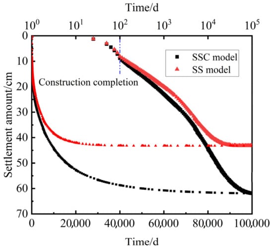
Figure 7.
Comparative settlement characteristics at the center of the subgrade determine from the SSC model and the SS model.
By comparing the calculation results of the two models, differences exist in the ratio of construction settlement to total settlement. For the SSC model, construction settlement accounts for 14.23% of total settlement, while for the SS model, construction settlement constitutes 18.75% of total settlement. Simultaneously, secondary consolidation settlement due to soft soil interlayer creep behavior can be determined. At 5655 days, 3.60 cm of secondary consolidation settlement occurs, accounting for 9.6% of the total settlement. Analysis of settlement development curves under both SSC and SS models shows that at 5655 days, the soil is in the mid-stage of consolidation. While the first soil layers to finish primary consolidation have entered secondary consolidation, most of the soil mass has not yet fully developed its secondary consolidation settlement.
4.3. Analysis of Pore Pressure Dissipation Characteristics and Strain Development Patterns
By the end of subgrade construction, the soil layers, excluding the soft soil interlayer within the foundation, had essentially completed primary consolidation and dissipation of the excess pore water pressure. Therefore, the C-1 and C-2 soil layers primarily influence the magnitude and rate of early settlement, particularly the immediate settlement. In contrast, the post-construction settlement magnitude and rate are mainly influenced by the S-1 soft soil interlayer [26].
Stress monitoring points were selected at the center of the subgrade and the middle of the S-1 soft soil interlayer to analyze the settlement and excess pore water pressure variations under different constitutive models. The analysis of the settlement and pore water pressure curves for the soft soil interlayer, as shown in Figure 8, reveals that during the rapid construction phase of the subgrade, pore water pressure rapidly accumulates due to the inadequate drainage condition of the foundation soil. The peak excess pore water pressure generated in the SSC constitutive model is 7.31% higher than that in the SS model, indicating that the compression of the soil is greater in the SSC model during the construction phase. From a temporal perspective, the maximum excess pore water pressure in the soft soil interlayer does not coincide with the completion of subgrade construction but exhibits a certain lag. This lag is more pronounced in the SSC model compared to the SS model. Analyzing the strain variation over time in the middle of the soft soil interlayer shows that strain development is faster in the SS model. This phenomenon occurs because the peak excess pore water pressure in the SS model is smaller and occurs earlier than in the SSC model, leading to the earlier dissipation of pore pressure in the middle of the soft soil interlayer, resulting in the compression of voids between soil particles and the subsequent strain.
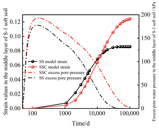
Figure 8.
Excess pore water pressure dissipation and strain curves of soil in the middle of the S-1 soft soil interlayer in the center of the subgrade.
As the operation time continues to increase, the excess pore water pressure gradually decreases, and by 20,000 days, the strain value of the soil in the SSC constitutive model will exceed that of the soil in the SS constitutive model. At 100,000 days, the strain value of the soil in the SSC model is 0.03857 higher than that in the SS model, accounting for 44.98% of the soil strain value in the SS model.
By comprehensively comparing the subgrade settlement and excess pore water pressure, it is evident that the settlement predictions and parameter calculations using the SSC constitutive model for the soft soil interlayer more accurately reflect the actual engineering conditions. Therefore, the subsequent analysis of settlement influenced by multiple factors is based on the SSC soft soil creep constitutive model.
4.4. Permeability Impact Analysis
The geotechnical properties of the interlayer soil significantly influence post-construction settlement. As the soil is a porous medium involving fluid–structure interaction, the consolidation process of the soft soil interlayer is significantly affected by different permeability coefficients [27,28].
The permeability coefficients of the soft soil interlayer are set to 5.75 × 10⁻⁵ m/d, 5.75 × 10⁻⁶ m/d, and 5.75 × 10⁻⁷ m/d, respectively. Stress nodes identical to those in Section 4.3 are selected to compare and analyze the differences in subgrade settlement and parameter variations under varying permeability conditions.
Figure 9 presents a comparison of the subgrade settlement under different permeability conditions. The settlement curves indicate that permeability significantly affects both the immediate settlement during construction and the post-construction settlement, but has minimal impact on the total settlement [29]. Specifically, for permeability parameters of 5.75 × 10⁻⁵, 5.75 × 10⁻⁶, and 5.75 × 10⁻⁷ m/d, the construction settlements are 14.30 cm, 8.81 cm, and 6.08 cm, respectively. The post-construction settlements are 48.27 cm, 53.38 cm, and 55.99 cm, respectively. This demonstrates that reducing permeability decreases immediate settlement while increasing the total post-construction settlement. Additionally, from the perspective of settlement stabilization time, reduced soil layer permeability significantly extends the duration required for settlement to stabilize [30,31]. This implies that soils with lower permeability dissipate the pore water pressure at a lower rate, leading to a prolonged settlement process. From a quantitative perspective, a tenfold decrease in the permeability coefficient results in the settlement stabilization time becoming 10.83 times longer than the original, while the post-construction settlement increases by an average of 7.74%.
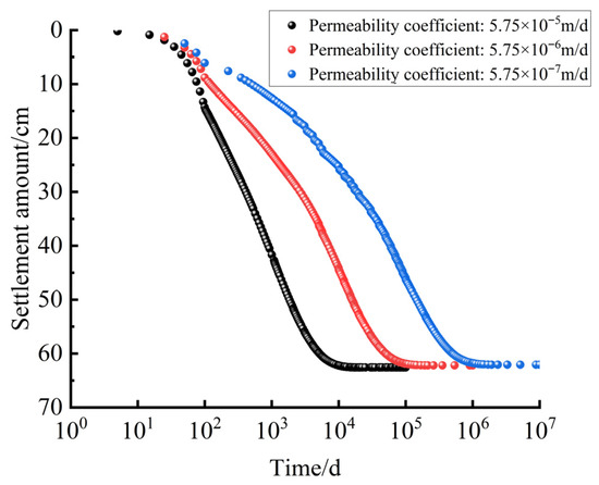
Figure 9.
Settlement curves of the subgrade center under different permeability coefficients of the S-1 soft soil interlayer.
4.5. Analysis of the Impact of Soft Soil Interlayer Thickness
The calculations indicate that the constitutive model and associated parameters of the S-1 soft soil interlayer are the primary factors determining subgrade settlement. According to the site investigation report, the thickness of the soft soil interlayer in the highway construction area ranges from 0.5 to 4 m. Therefore, it is essential to explore the impact of soft soil interlayer thickness on subgrade settlement. In this analysis, finite element models with varying thicknesses of the soft soil interlayer were established. The geotechnical properties for each layer remain consistent, while the soft soil layer is assigned a permeability coefficient of 5.75 × 10⁻⁶ m/d and a depth of 5 m. It is conducted to investigate the effects of soft soil interlayer thickness on settlement magnitude and stabilization time. Figure 10 shows the settlement variation curves at the subgrade center for different soft soil interlayer thicknesses, and Figure 11 presents the fitting curves for settlement magnitude, settlement time (representing 95% of the total settlement), and soft soil interlayer thickness.
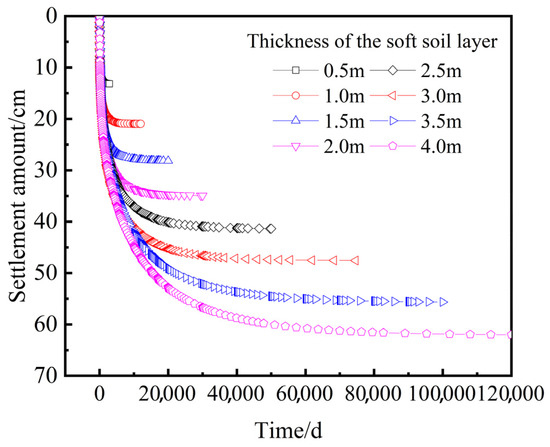
Figure 10.
Settlement curves of the subgrade center under different thicknesses of soft soil interlayer.
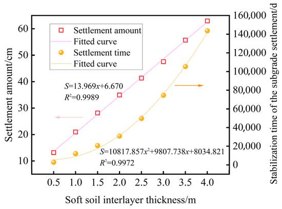
Figure 11.
Relationships of the thickness of soft soil interlayer with settlement and settling time.
Figure 10 illustrates that as the thickness of the soft soil interlayer increases, both the final settlement and the time required for settlement stabilization significantly increase. During the initial phase, the settlement trends for soft soil interlayers of varying thicknesses are nearly identical. However, the settlement rate for thinner soft soil interlayers gradually decreases over time, while thicker soft soil interlayers exhibit a continual increase in settlement to achieve an equilibrium condition. This indicates that, during long-term consolidation, the compression of the soil and dissipation of pore water pressure extend progressively from the interface between the soft soil interlayer and the silty clay layer into the interior of the interlayer, as shown in Figure 12, until a new equilibrium state is reached. This phenomenon corroborates the strain development patterns discussed in Section 4.3. It reflects the significant impact of soft soil interlayer thickness on settlement behavior and highlights the crucial role of the pore water pressure dissipation process in the consolidation process.
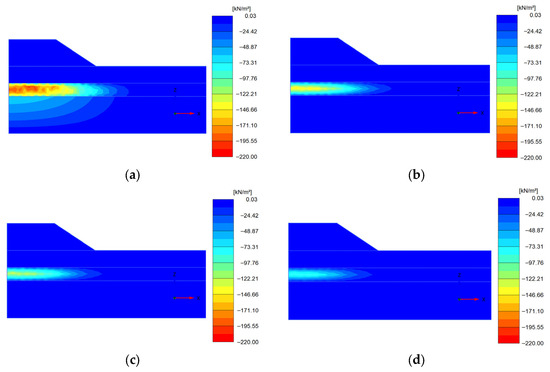
Figure 12.
Excess pore water pressure dissipation cloud map obtained after: (a) 100 days; (b) 5655 days; (c) 10,000 days; (d) 20,000 days.
Figure 11 indicates that the settlement magnitude exhibits a linear relationship with the thickness of the soft soil interlayer; thicker soft soil interlayers result in greater settlement. In contrast, the settlement time follows a quadratic function with respect to the soft soil interlayer thickness, with an increase in thickness significantly prolonging the stabilization time of the subgrade settlement. When the thickness of the soft soil interlayer increases from 0.5 m to 4 m, the final settlement becomes 4.78 times greater than the original value, and the settlement stabilization time becomes 50.39 times longer.
4.6. Analysis of the Impact of Soft Soil Interlayer Depth
Since the subgrade section features a typical sandwich soil layer structure, with consistent soil parameters, the geometrical parameters of the foundation soil play a critical role in controlling consolidation. Therefore, based on a finite element model with a 4-m-thick soft soil interlayer, the impact of the depth of the soft soil interlayer on foundation settlement characteristics was investigated by varying the thickness of the overlying silty clay layer (C-1). Figure 13 illustrates the variation in settlement at the subgrade center under different soft soil interlayer depths, as well as the functional relationship between the final settlement and the burial depth of the soft soil interlayer.
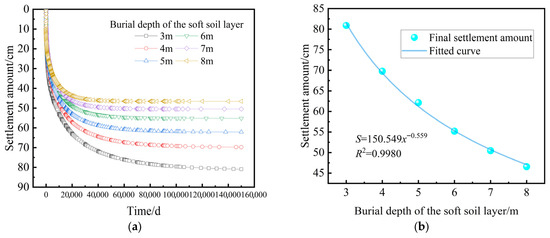
Figure 13.
Settlement characteristics at the subgrade centerline: (a) settlement curves under different burial depths of the soft soil interlayer; (b) functional relationship between the burial depth of the soft soil interlayer and the final settlement.
Figure 13 shows that as the depth of the soft soil interlayer increases, the final settlement decreases significantly, but this relationship is not linear. Within a certain depth range, the rate of reduction in final settlement decreases as the depth of the soft soil interlayer increases. When the burial depth of the soft soil interlayer increases from 3 m to 8 m, the final settlement decreases by approximately 42.44%. During the initial phase, the settlement trends for soft soil interlayers at different depths are nearly identical. However, over time, the settlement rate for deeper soft soil interlayers gradually slows down, while shallower soft soil interlayers continue to experience compression until they reach stabilization, with minimal differences in the final settlement stabilization time.
4.7. Analysis of the Impact of Subgrade Height
During highway operation, the long-term load applied to the foundation soil is the self-weight of the subgrade. For a constant subgrade width and slope, varying embankment heights result in different magnitudes of load on the foundation. Therefore, the height of the subgrade has a significant impact on the overall coordinated deformation of the foundation. In this analysis, finite element models with a 4-m-thick soft soil interlayer and a 5-m depth were used. By setting different embankment heights, the effects of embankment height on foundation settlement magnitude and stabilization time were computed and analyzed.
Figure 14 illustrates that as the subgrade fill height increases, both the final settlement magnitude and the time required for settlement significantly increase. When the embankment height increases from 2 m to 10 m, the final settlement increases by approximately 379.14%. The settlement magnitude exhibits a nearly linear relationship with embankment height, and the embankment height has a more significant influence on the final settlement compared to the thickness and depth of the soft soil interlayer. During the initial phase, the settlement trends for different embankment heights are almost identical. However, over time, the settlement rate for lower embankment heights gradually decreases, while higher embankment heights continue to experience compression until stabilization is achieved.
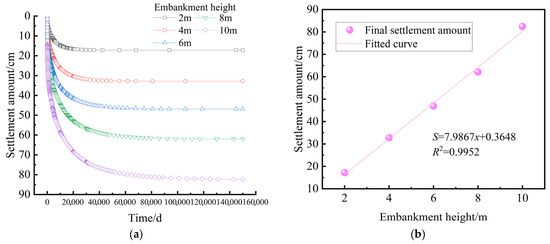
Figure 14.
Settlement characteristics at the subgrade centerline: (a) settlement curves under different embankment heights; (b) functional relationship between embankment height and final settlement.
The service life of the highway subgrade is sufficient at 20,000 days. Under the condition of a 4 m thick soft soil interlayer, the settlement of the subgrade over 20,000 days is influenced by both the burial depth of the soft soil interlayer and the embankment height, as shown in Figure 15. Overall, the embankment height has a greater impact on the settlement amount than the burial depth of the soft soil interlayer. When the burial depth of the soft soil interlayer is shallow and the embankment height is high, the settlement increases substantially. Conversely, when the burial depth of the soft soil interlayer is deep and the embankment height is low, the settlement increases gradually.
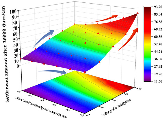
Figure 15.
Combined effect of the burial depth of the soft soil interlayer and embankment height on the settlement.
To address the critical issues arising from insufficient field settlement monitoring data, such as inaccurate subgrade settlement predictions, unclear multi-factor interactions, challenges in quantitative analysis of impact severity, and diverse soil layer structures in subgrade sections, a deep learning network is established to achieve comprehensive and precise prediction of subgrade settlement.
5. Prediction of Pavement Settlement Across Entire Sections and Operational Periods Using a Genetic Algorithm-Optimized Backpropagation Neural Network (GA-BP)
5.1. Construction of the Neural Network Model
The backpropagation neural network (BP) consists mainly of an input layer, hidden layers, and an output layer, as shown in Figure 16. The input layer receives data, the hidden layers perform feature extraction, and the output layer generates results. Its advantages include the ability to handle complex nonlinear problems, strong adaptability, and automatic optimization of the model through learning, making it suitable for various tasks such as regression and classification [32]. Additionally, genetic algorithms (GA) have strong global search capabilities, so GA is introduced to optimize the initial parameters of the BP neural network [33]. The process of optimizing a Backpropagation (BP) neural network using a genetic algorithm can be divided into three main modules: determining the optimization parameters for the genetic algorithm, defining the topology of the BP neural network, and implementing the prediction functionality of the BP neural network [34]. The detailed process is illustrated in Figure 17.
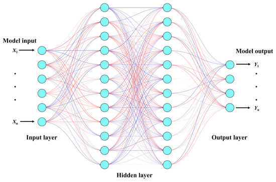
Figure 16.
Schematic Diagram of the BP Neural Network Architecture.
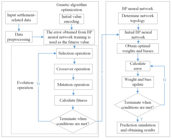
Figure 17.
GA-BP neural network subgrade settlement intelligent prediction process.
Optimizing the parameters of the neural network, specifically the weights and biases, involves encoding them using a genetic algorithm to generate an initial population, with each individual carrying specific weight and bias information [35]. During the optimization process, the genetic algorithm iteratively improves the performance of individuals in the population through selection, crossover, and mutation operations, enhancing their performance on training data. After multiple iterations, the algorithm converges to the optimal or near-optimal solution, resulting in the optimized weights and biases for the BP neural network [36]. The topology of the BP neural network is determined, including the number of input and output parameters, the number of weights for the input and output layers, and the number of biases for the hidden and output layers. Based on this topological information, the encoding length for the genetic algorithm individuals is established. The optimized BP neural network is then used for regression tasks, significantly improving the model’s generalization ability and prediction accuracy. Genetic algorithm optimization not only enhances the training effectiveness of the BP neural network but also overcomes the limitation of the algorithm’s tendency to fall into local optima, thus significantly improving the overall performance of the neural network.
5.2. Establishment of Training and Testing Datasets
This regression prediction model is implemented using MATLAB R2023b. It utilizes settlement data obtained from numerical simulations to prepare the input and output data for the model. Specifically, five parameters—road embankment height, soft soil interlayer thickness, soft soil interlayer depth, settlement time, and distance from the settlement monitoring points to the centerline—are used as input variables, while the corresponding subgrade settlement values for each set of input data are used as output variables. The specific values of each input parameter are detailed in Table 5. The schematic diagram of the distance from the settlement monitoring point on the top surface to the centerline is shown in Figure 18. The dataset consists of a total of 10,747 samples. Among them, 10,718 samples with subgrade heights of 2 m, 4 m, 6 m, and 10 m were used as the training set, while 29 samples with a subgrade height of 8 m were used as the test set for validation analysis. The prediction is carried out using a genetic algorithm-optimized BP neural network, where the absolute error of the training dataset is used as the fitness value for the test individuals. The individual with the smallest fitness value is ultimately selected for prediction calculations to ensure the accuracy and reliability of the results [37].
Table 5.
GA-BP input parameter.
Figure 18.
Schematic diagram of the distance from the surface settlement monitoring point to the subgrade centerline (unit: m).
5.3. Network Configuration and Model Accuracy Evaluation Methods
The network is configured with one hidden layer comprising 5 neurons. The parameters for the genetic algorithm are set as follows: initial population size of 50, evolution generations of 100, crossover probability of 0.4, mutation probability of 0.04, maximum number of iterations set to 1000, learning rate of 0.01, and a training target error threshold of 1 × 10⁻⁶. Training is terminated once the specified criteria are met, ensuring that the algorithm maintains a sufficient level of global search capability even after significant progress has been achieved.
To evaluate the accuracy of the prediction model, it is necessary to consider the errors in both the test set and the training set. This study employs Root Mean Square Error (RMSE) and Mean Absolute Percentage Error (MAPE) to assess the accuracy of the GA-BP neural network model [38], and the calculation method is consistent with Equations (8) and (9). Additionally, the coefficient of determination R2 is used to evaluate the fitting performance of the training set [39]. The calculation formula is as follows.
In the formula, represents the simulated settlement value at time t; represents the predicted settlement value at time t; n is the number of samples in the dataset; and denotes the mean of the n simulated settlement values. The smaller the Root Mean Square Error (RMSE) and Mean Absolute Percentage Error (MAPE), combined with a coefficient of determination (R2) closer to 1, indicates higher the prediction accuracy of the GA-BP model on the training.
The fitness value variation curve of the BP neural network prediction model optimized by the genetic algorithm is shown in Figure 19. As the number of iterations increases, the fitness value continuously decreases in a stepwise manner, indicating that the model’s prediction performance improves gradually, and the individuals in the population converge toward the global optimal solution [40]. The figure shows that after 35 iterations, the fitness value decreases from 0.01569 to 0.01476. After this point, the fitness value stabilizes and no significant changes occur with further iterations, indicating that the algorithm has converged to a relatively ideal solution.
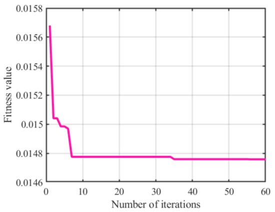
Figure 19.
Fitness value variation curve.
5.4. Analysis of Full-Section and Full-Cycle Pavement Settlement Prediction Results
The original data with embankment heights of 2 m, 4 m, 6 m, and 10 m were selected as the training set, while data with an 8 m embankment height, 4 m soft soil interlayer thickness, and 5 m soft soil depth were used as the test set. The test set includes data on the settlement of this typical cross-section as it varies with time and distance from the centerline. Given the inherent randomness in neural network training, predictions were averaged over 10 calculations to obtain the output. Model training is shown in Figure 20, with errors summarized in Table 6.
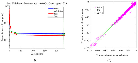
Figure 20.
Model Training and Establishment: (a) Network training process. (b) Fit of predictive model.
Table 6.
Details of performance indices during the training and testing of the model.
The training results of the GA-BP neural network model indicate an RMSE of 0.01826 m, an MAPE of 6.1610%, and a coefficient of determination R2 of 0.9864. For the testing results, the model yields an RMSE of 0.01488 m, an MAPE of 7.0562%, and a coefficient of determination R2 of 0.9706. The predicted settlement over time at the centerline for an 8 m embankment height, 4 m soft soil interlayer thickness, and 5 m soft soil depth is shown in Figure 21. The predicted settlement in the transverse spatial dimension at 5655 days for the same parameters is depicted in Figure 22. These results demonstrate that the developed model effectively predicts settlement data that vary with both time and spatial dimensions. By integrating the subgrade settlement data obtained from numerical simulations and based on the GA-BP neural network model, an effective solution was provided for the full life cycle and three-dimensional full-section precise prediction of subgrade settlement under the influence of multiple factors in soft soil interlayer foundations. This enriched the predictive experience database for subgrade settlement on soft soil interlayer foundations and provided valuable insights for similar engineering projects under the same environmental conditions.
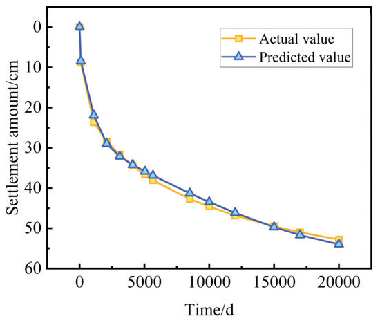
Figure 21.
Comparison of settlement behavior against time.
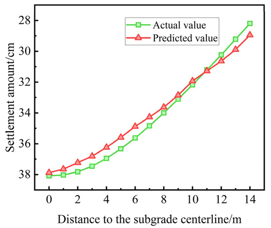
Figure 22.
Comparison of settlement behavior across the lateral spatial dimension.
6. Conclusions
This study established a subgrade settlement calculation model for soft soil interlayer foundations in the Yellow River floodplain using finite element numerical simulation. The model’s reliability was verified with field monitoring data, and the multi-factor influence of soft soil interlayers on embankment settlement was systematically analyzed. By integrating numerical simulation results with neural network techniques, a genetic algorithm–optimized backpropagation neural network (GA-BP) settlement prediction model was developed. The main findings are as follows:
- (1)
- Compared with the SS constitutive model, the SSC constitutive model more effectively simulates the secondary consolidation characteristics of soft soil interlayers, and the proportion of secondary consolidation settlement increases over time.
- (2)
- The choice of constitutive model affects the proportion of settlement occurring during construction: in the SSC model, construction-period settlement accounts for 14.23% of the total settlement, whereas in the SS model, this proportion reaches 18.75%.
- (3)
- Excess pore pressure dissipates progressively from the soft soil–silty clay interface to equilibrium. Lower permeability in the soft interlayer prolongs settlement stabilization and increases post-construction settlement. A tenfold permeability reduction makes stabilization 10.83 times longer and raises post-construction settlement by 7.74%.
- (4)
- The final settlement increases linearly with the soft interlayer thickness and embankment height, but decreases as a power function with greater interlayer depth. The stabilization time shows a quadratic relation with interlayer thickness and is little affected by interlayer depth or embankment height.
- (5)
- The proposed GA-BP model incorporates multiple influencing factors and considers the transverse spatial variability of the subgrade. The model achieved an RMSE of 0.01826 m, MAPE of 6.1610%, and R2 of 0.9864 for the training dataset, and an RMSE of 0.01488 m, MAPE of 7.0562%, and R2 of 0.9706 for the testing dataset.
The developed model can be applied to predict the long-term settlement of soft soil subgrades under temporal and spatial variations. However, its applicability is somewhat limited due to factors such as soil conditions and the exclusion of vehicle loads. Future studies could investigate the effects of soil variability and traffic load uncertainties on consolidation settlement.
Author Contributions
Conceptualization, Y.L. and T.L.; methodology, K.Y.; software, A.Z.; validation, Z.Y.; formal analysis, L.Z.; investigation, Z.S. (Zhaoyun Sun); resources, X.X.; data curation, Y.L. and L.Z.; writing—original draft, Y.L. and A.Z.; writing—review and editing, Z.S. (Zihan Sang), K.Y. and Z.Y.; visualization, T.L.; project administration, X.X.; funding acquisition, K.Y. All authors have read and agreed to the published version of the manuscript.
Funding
This research was funded by Shandong Provincial Natural Science Foundation (ZR2024LZN002), Shenzhen Science and Technology Program (SZXJP20230703093002005), and Jinan Science & Technology Bureau Project (202333051).
Data Availability Statement
The data supporting the conclusions of this study are included in this article. For further inquiries, please contact the corresponding authors directly.
Conflicts of Interest
Authors Yong Lu, Xianjin Xu and Tao Lei were employed by Qilu Expressway Company Limited. The remaining authors declare that the research was conducted in the absence of any commercial or financial relationships that could be construed as a potential conflict of interest.
References
- Navarro, V.; Asensio, L.; Alonso, J.; Yustres, Á.; Pintado, X. Multiphysics Implementation of Advanced Soil Mechanics Models. Comput. Geotech. 2014, 60, 20–28. [Google Scholar] [CrossRef]
- Hirai, H. Settlements and Stresses of Multi-Layered Grounds and Improved Grounds by Equivalent Elastic Method. Int. J. Numer. Anal. Methods Geomech. 2008, 32, 523–557. [Google Scholar] [CrossRef]
- Liu, Z. Research and Engineering Application of Roadbed Settlement Prediction Method Based on Measured Data. In Water Conservancy and Civil Construction Volume 2; CRC Press: Boca Raton, FL, USA, 2023; ISBN 978-1-003-45083-2. [Google Scholar]
- ACAR, Y.; HILAL, H.; TUMAY, M. Fem Analysis of Elastic Stress Distributions in Embankments. J. Geotech. Eng. ASCE 1988, 114, 711–718. [Google Scholar] [CrossRef]
- Lan, T.; Wang, J. Settlement Prediction and Differential Settlement Criterion for Heightening and Thickening Levee. Appl. Sci. 2018, 8, 2392. [Google Scholar] [CrossRef]
- Li, C. A Simplified Method for Prediction of Embankment Settlement in Clays. J. Rock Mech. Geotech. Eng. 2014, 6, 61–66. [Google Scholar] [CrossRef]
- Zhou, C.; Yu, L.; Huang, Z.; Liu, Z.; Zhang, L. Analysis of Microstructure and Spatially Dependent Permeability of Soft Soil during Consolidation Deformation. SOILS Found. 2021, 61, 708–733. [Google Scholar] [CrossRef]
- Khan, M.U.A.; Shukla, S.K.; Raja, M.N.A. Load-Settlement Response of a Footing over Buried Conduit in a Sloping Terrain: A Numerical Experiment-Based Artificial Intelligent Approach. Soft Comput. 2022, 26, 6839–6856. [Google Scholar] [CrossRef]
- Díaz, E.; Tomás, R. Revisiting the Effect of Foundation Embedment on Elastic Settlement: A New Approach. Comput. Geotech. 2014, 62, 283–292. [Google Scholar] [CrossRef]
- Díaz, E.; Tomás, R. A Simple Method to Predict Elastic Settlements in Foundations Resting on Two Soils of Differing Deformability. Eur. J. Environ. Civ. Eng. 2016, 20, 263–281. [Google Scholar] [CrossRef]
- Hsieh, P.; Ou, C. Shape of Ground Surface Settlement Profiles Caused by Excavation. Can. Geotech. J. 1998, 35, 1004–1017. [Google Scholar] [CrossRef]
- Li, Z.; Peng, Y.; Li, J.; Tang, Z. Composite Foundation Settlement Prediction Based on LSTM–Transformer Model for CFG. Appl. Sci. 2024, 14, 732. [Google Scholar] [CrossRef]
- Li, G.H.; Liu, H.B.; Qin, X.X. Settlement Prediction of Roadbed Based on Mixture Model with Exponential Curve and ANN. Adv. Mater. Res. 2013, 663, 76–79. [Google Scholar] [CrossRef]
- Hui, G.; Qi-chao, S.; Jun, H. Application of twin support vector regression in subgrade settlement prediction. Int. J. u- e-Serv. Sci. Technol. 2016, 9, 101–108. [Google Scholar] [CrossRef]
- Huang, C.; Li, Q.; Wu, S.; Li, J.; Xu, X. Application of the Richards Model for Settlement Prediction Based on a Bidirectional Difference-Weighted Least-Squares Method. Arab. J. Sci. Eng. 2018, 43, 5057–5065. [Google Scholar] [CrossRef]
- Huang, L.; Qin, W.; Dai, G.; Zhu, M.; Liu, L.-L.; Huang, L.-J.; Yang, S.-P.; Ge, M.-M. Ground Settlement Prediction for Highway Subgrades with Sparse Data Using Regression Kriging. Sci. Rep. 2024, 14, 24594. [Google Scholar] [CrossRef] [PubMed]
- Zhang, J. Research on Application of Intelligent Monitoring Technology in Highway Subgrade Settlement Prediction. In Frontiers in Artificial Intelligence and Applications; Jain, L.C., Balas, V.E., Wu, Q., Shi, F., Eds.; IOS Press: Amsterdam, The Netherlands, 2025; ISBN 978-1-64368-586-1. [Google Scholar]
- Xie, S.-L.; Hu, A.; Wang, M.; Xiao, Z.-R.; Li, T.; Wang, C. 1DCNN-Based Prediction Methods for Subsequent Settlement of Subgrade with Limited Monitoring Data. Eur. J. Environ. Civ. Eng. 2025, 29, 759–784. [Google Scholar] [CrossRef]
- Wang, L.; Li, T.; Wang, P.; Liu, Z.; Zhang, Q. BiLSTM for Predicting Post-Construction Subsoil Settlement under Embankment: Advancing Sustainable Infrastructure. Sustainability 2023, 15, 14708. [Google Scholar] [CrossRef]
- Berre, S. Back Calculation of Measured Settlements for an Instrumented Fill on Soft Clay. Master’s Thesis, Norwegian University of Science and Technology (NTNU), Trondheim, Norway, 2017. [Google Scholar]
- Waheed, M.Q.; Asmael, N.M. Using Soft Soil Models in Geotechnical Engineering: A Review Paper. E3S Web Conf. 2024, 531, 04018. [Google Scholar] [CrossRef]
- Kumar Thota, S.; Duc Cao, T.; Vahedifard, F. Poisson’s Ratio Characteristic Curve of Unsaturated Soils. J. Geotech. Geoenviron. Eng. 2021, 147, 04020149. [Google Scholar] [CrossRef]
- Sivasithamparam, N.; Karstunen, M.; Bonnier, P. Modelling Creep Behaviour of Anisotropic Soft Soils. Comput. Geotech. 2015, 69, 46–57. [Google Scholar] [CrossRef]
- Peduto, D.; Prosperi, A.; Nicodemo, G.; Korff, M. District-Scale Numerical Analysis of Settlements Related to Groundwater Lowering in Variable Soil Conditions. Can. Geotech. J. 2022, 59, 978–993. [Google Scholar] [CrossRef]
- Wei, Z.; Zhu, Y. A Theoretical Calculation Method of Ground Settlement Based on a Groundwater Seepage and Drainage Model in Tunnel Engineering. Sustainability 2021, 13, 2733. [Google Scholar] [CrossRef]
- Salem, M.; El-Sherbiny, R. Comparison of Measured and Calculated Consolidation Settlements of Thick Underconsolidated Clay. Alex. Eng. J. 2014, 53, 107–117. [Google Scholar] [CrossRef]
- Xie, K.; Xia, C.; An, R.; Ying, H.; Wu, H. A Study on One-dimensional Consolidation of Layered Structured Soils. Int. J. Numer. Anal. Methods Geomech. 2016, 40, 1081–1098. [Google Scholar] [CrossRef]
- Zhou, Y.; Lai, Y.; Chen, X.; Han, X.; Peng, Y. Research on Consolidation and Settlement Characteristics of Soft Soil with High Initial Water Content. J. Ocean Eng. Mar. Energy 2025, 11, 467–481. [Google Scholar] [CrossRef]
- Zeng, Y. Geotechnical Settlement Deformation Analysis of Soft Sub-Grade Embankment Filling Construction Period Based on Unified Hardening Model. Geotech. Geol. Eng. 2019, 37, 5473–5483. [Google Scholar] [CrossRef]
- Zhang, M.; Zhu, X.; Yu, G.; Yan, J.; Wang, X.; Chen, M.; Wang, W. Permeability of Muddy Clay and Settlement Simulation. Ocean Eng. 2015, 104, 521–529. [Google Scholar] [CrossRef]
- Zhou, S.; Wang, B.; Shan, Y. Review of Research on High-Speed Railway Subgrade Settlement in Soft Soil Area. Railw. Eng. Sci. 2020, 28, 129–145. [Google Scholar] [CrossRef]
- Buscema, M. Back Propagation Neural Networks. Subst. Use Misuse 1998, 33, 233–270. [Google Scholar] [CrossRef]
- Sexton, R.S.; Dorsey, R.E.; Johnson, J.D. Toward Global Optimization of Neural Networks: A Comparison of the Genetic Algorithm and Backpropagation. Decis. Support Syst. 1998, 22, 171–185. [Google Scholar] [CrossRef]
- Ding, S.; Su, C.; Yu, J. An Optimizing BP Neural Network Algorithm Based on Genetic Algorithm. Artif. Intell. Rev. 2011, 36, 153–162. [Google Scholar] [CrossRef]
- Abdolrasol, M.G.M.; Hussain, S.M.S.; Ustun, T.S.; Sarker, M.R.; Hannan, M.A.; Mohamed, R.; Ali, J.A.; Mekhilef, S.; Milad, A. Artificial Neural Networks Based Optimization Techniques: A Review. Electronics 2021, 10, 2689. [Google Scholar] [CrossRef]
- Lee, S.; Kim, J.; Kang, H.; Kang, D.-Y.; Park, J. Genetic Algorithm Based Deep Learning Neural Network Structure and Hyperparameter Optimization. Appl. Sci. 2021, 11, 744. [Google Scholar] [CrossRef]
- Wilson, S.W. Classifier Fitness Based on Accuracy. Evol. Comput. 1995, 3, 149–175. [Google Scholar] [CrossRef]
- Liu, C.Y.; Wang, Y.; Hu, X.M.; Han, Y.L.; Zhang, X.P.; Du, L.Z. Application of GA-BP Neural Network Optimized by Grey Verhulst Model around Settlement Prediction of Foundation Pit. Geofluids 2021, 2021, 5595277. [Google Scholar] [CrossRef]
- Chicco, D.; Warrens, M.J.; Jurman, G. The Coefficient of Determination R-Squared Is More Informative than SMAPE, MAE, MAPE, MSE and RMSE in Regression Analysis Evaluation. PeerJ Comput. Sci. 2021, 7, e623. [Google Scholar] [CrossRef]
- Pandey, H.M.; Chaudhary, A.; Mehrotra, D. A Comparative Review of Approaches to Prevent Premature Convergence in GA. Appl. Soft Comput. 2014, 24, 1047–1077. [Google Scholar] [CrossRef]
Disclaimer/Publisher’s Note: The statements, opinions and data contained in all publications are solely those of the individual author(s) and contributor(s) and not of MDPI and/or the editor(s). MDPI and/or the editor(s) disclaim responsibility for any injury to people or property resulting from any ideas, methods, instructions or products referred to in the content. |
© 2025 by the authors. Licensee MDPI, Basel, Switzerland. This article is an open access article distributed under the terms and conditions of the Creative Commons Attribution (CC BY) license (https://creativecommons.org/licenses/by/4.0/).