1. Introduction and State of the Art
Model-based damage identification approaches, which rely on finite element method-built models, are particularly popular, especially when it comes to damage localization and quantification [
1,
2]. With these approaches, simulated models are excited like their corresponding experimental structures and the real structure itself. The output is then observed and compared to the collected experimental results. The disparity in the responses is minimized by formulating an inverse problem, followed by the updating of the identified potential parameters that encapsulate the information change [
3,
4,
5,
6,
7]. In this regard, natural frequency and modal parameters are the most commonly extracted features to indicate damage [
8,
9]. The primary challenge associated with this approach is the difficulty in obtaining a reliable simulated model that accurately matches the corresponding experimental model [
10].
A comparable approach, fundamentally dependent on statistical analysis and pattern recognition, is the data-driven method. In contrast to the model-based approach, there is no need for a real- structure-representing simulated model. Instead, datasets collected from the target structure using sensors are processed to identify trends, recognize patterns, and observe statistical measurements [
11,
12,
13,
14,
15]. These extracted features will be used to train machine learning models and make acceptable predictions. Models trained with a data-driven approach, however, usually demand larger datasets [
16,
17,
18]. The larger the dataset, with due consideration given to its quality, the better the model will be.
Damage identification encompasses damage detection, localization, type, severity, and remaining lifetime prediction [
1,
19]. The first four steps constitute the diagnosis category. The fifth step, which usually is a prognosis, requires historical data and experience from similar structures and thus is not a simple task.
In a machine learning-based structural health monitoring (SHM) damage identification process, there are several essential steps, from data collection to damage prediction. The key intermediate steps include dataset preprocessing, feature extraction, dimensionality reduction, and model training [
20,
21].
Ref. [
22] employed data-driven one-dimensional convolutional neural network (CNN) and recurrent neural network (RNN) models to directly learn from time series signals. These signals, typically collected for vibration-based damage identification purposes, inherently possess sequence dependencies. They implemented an attention layer to compute attention weights for each input. A framework for damage identification was developed using a support vector machine (SVM) in [
23]. They applied the wavelet transform, Hilbert–Huang transform, and Teager–Huang transform to diagnose a cable-stayed bridge, accounting for environmental variability. A data-driven damage localization approach [
24] and the probabilistic quantification and assessment of prediction errors in damage detection [
25] are some of the achievements made in data-driven structural damage identification.
Ref. [
26] applied time-domain machine learning techniques to deal with environmental and operational effects (EOFs). They also extended their efforts to deal with autoregressive-based extrapolation approaches. This dataset is used in our current study.
Environmental effects, such as temperature variations, and operational effects, like traffic loading, have been identified as significant factors that greatly impact the damage identification process [
16,
27]. While not being direct indicators of damage, these effects exhibit trends similar to those caused by damage. They influence characteristics such as the mass and stiffness of structural members, consequently altering the natural frequencies. This phenomenon makes the activity of damage detection even more challenging.
Regression models [
28], blind source separation techniques [
29], the Mahalanobis squared distance [
30,
31], principal component analysis (PCA), and factor analysis have been implemented to treat environmental and operational effects [
32]. Extensive works on damage identification, modeling approaches, and EOF treatment may be found in [
33,
34,
35,
36,
37,
38,
39].
The features used to train machine learning models might be mined from different domains. Though time-domain [
40] approaches like autoregression (AR), autoregression moving average (ARMA), and autoregression moving average with exogenous inputs (ARMAX) are preferred for their simplicity, for complex tasks, however, frequency-domain approaches such as the fast Fourier transform (FFT) [
41] and time-and-frequency-domain approaches like the wavelet transform (WT) [
23,
42] are popular. As feature extraction and selection approaches have a crucial role in machine learning models, such areas of study constantly draw the attention of researchers.
The primary objective of this paper is to investigate the impact of various FFT- and WT-based features on machine learning models, such as neural networks (NNs) and recurrent neural networks (RNNs). Additionally, the paper proposes a comparable feature extraction/selection technique that can mitigate the influence of EOFs with reduced computational effort. The study extends its focus to include damage localization and severity assessment.
In this research, supervised machine learning models are trained using multiple features extracted from the acceleration signals of a three-story frame modeled in the Los Alamos laboratory, while considering the presence of EOFs. The effects of EOFs on this dataset were previously examined and successfully addressed using a time-domain approach involving autoregression and a statistical tool, the Mahalanobis distance [
26]. In our study, however, FFT and WT coefficients are used separately to train both NN and RNN models. Additionally, different WT coefficients and their combinations are tested to produce better-quality models.
A sensitivity analysis of signal segmentation, the overlapping length, training dataset imbalance treatment, and PCA usage for both dimension reduction and EOF treatment is also conducted on different combinations of features. Subsequently, leveraging the maximum change detection concept, a feature extraction/selection approach is developed and implemented. This method identifies the most damage-sensitive segment (MDSS) from each signal based on the maximum difference criterion of each selected feature variable, returning the associated coefficients as learning features. The results of this approach demonstrate improvements compared to the direct use of FFT and multiple WT-based features.
The remainder of this work is structured as follows. Initially, the damage detection process is elucidated, detailing the methods implemented in the study. Subsequently, the dataset utilized, acquired from four sensors, is outlined. Various approaches to replacing missing signals are considered, and the optimal method is selected. In the subsequent feature extraction section, coefficients from FFT and WT are extracted, with different sensitivity analyses conducted. The MDSS selection approach is introduced and discussed.
Following this, both binary and multiclass classification supervised machine learning models are trained, and their performance is evaluated. The damage detection, localization, and severity assessment are then examined. Severity labels are assigned based on insights derived from statistical computations of the FFT coefficients. The effects of oversampling and undersampling are also observed and discussed. Python 3.8.17 and Tensorflow 2.13.0 together with all machine learning libraries are used on Jupyter Notebook 7.0.8 for the training of the models and all related tasks. The desktop computer runs on the 64-bit Windows 10 operating system, with a 12th Gen Core i7 processor, with 3.63 TB storage and 32 GB RAM.
2. Damage Detection, Research Design, and Dataset Description
2.1. Damage Detection Process
The damage detection process primarily comprises two phases: the model creation phase and the prediction phase. In the model creation phase, data preparation—in this paper, involving the replacement of missing data and data normalization—is a crucial step. Subsequently, features are extracted to facilitate the training of the machine learning models. In this regard, potential features that can capture the trends and recognize the patterns, such as the FFT and WT coefficients, are used [
43]. To address the high dimensionality of these coefficients and enhance the training speed while reducing the computational demands, an unsupervised PCA method is implemented [
44]. Before training the model, the dataset used is balanced for the assigned labels. In this work, for binary classification, for example, the number of signals for the damaged and undamaged states of the given structure is balanced. For this purpose, both manual and SMOTE approaches are used [
45]. Then, the NN and RNN models are trained and tested [
34,
37].
In the prediction phase, the damage detection approach classifies structural conditions as damaged and undamaged. The damage identification process, however, includes damage localization, identifying the location of the potential damage, the damage severity, and the extent of the damage. The flow chart in
Figure 1 illustrates mainly the damage detection process with the methods implemented in this study. The MDSS, however, does not require dimensionality reduction methods such as PCA as it has less dimensionality, which corresponds to the types of coefficients extracted from the PSD plot (only twenty coefficients).
2.2. Research Design
Structures in the real world are exposed to multiple variabilities. Vibration-based sensors are preferred for their potential to capture the global response of a given structure are therefore expected to return signals capturing these variabilities. Accordingly, the dataset used in this work consists of signals representing four conditions: healthy, with EOFs, damaged, and damaged with EOFs.
To detect damage from the given conditions and thereby treat EOFs, multiple features ranging from the time to the time–frequency domains are extracted. The four condition signals are studied using coherence and PSD plots to capture meaningful patterns. Based on the observations from the PSD plots of the sample signals from all four conditions, the MDSS technique is developed and implemented. This technique searches for the most sensitive segment from each signal for a specified feature coefficient.
Figure 2 shows the research approach followed in this paper. In both cases, the approach is data-driven damage detection using ML models. In the left-hand approach, features are extracted based on time-domain, frequency-domain, and time–frequency domain coefficients. In the right-hand approach, however, sample signals from four different conditions are first studied with coherence and PSD plots regarding whether they contain underlying patterns that differentiate them from each other. Based on the observed potential, the MDSS technique is devised to extract better-quality coefficients from each of the most damage-sensitive segments in the frequency domain. Details are included in the respective sections.
2.3. Dataset Description
The dataset is taken from the Los Alamos National Laboratory, USA [
46]. A test on a three-story building structure was conducted to detect nonlinear effects. Out of 24 states of the test, only 17 states were considered as complete and made available online.
The 17 states represent four different conditions or exposures of the building structure. These include undamaged, with EOFs, damaged, and with EOFs and damage combined. Signals from the undamaged state serve as a baseline for further processing. Signals collected under the influence of EOFs are simulated with a column stiffness reduction for environmental effects and a floor weight increment for operational effects, respectively.
Damage is introduced through an impact load applied with a bumper to a hanging column, thereby affecting the entire structure. The magnitude of the damage is determined by the gap size between the bumper and the hanging column. A larger gap size corresponds to a higher damage level. The gap sizes used in the conducted experiment are 0.05 mm, 0.1 mm, 0.13 mm, 0.15 mm, and 0.2 mm. Nonlinearity to the extent of resulting damage is induced by a bumper.
Each state consists of ten test trials. Each test trial has four acceleration sensor records, one on each floor. The sampling frequency and frequency resolution are 322.58 Hz and 0.039 Hz, respectively. There are thus 8192 data points in every signal. Details of the model and collected dataset can be found in [
26].
Table 1 shows the four condition categories and the number of states in each category, with a single state containing ten files of signals from four sensors. The dataset’s signals are arranged in rows, while their data points are in columns. This forms a table with a size of 676 by 8192. This is due to one missed file (signal records from four sensors) from the undamaged condition of the dataset.
2.4. Dataset Normalization
Dataset normalization is used to bring all the signals to the same scale and thereby avoid discrepancies, reduce noise, and reduce the computational load. Outliers can also be identified using a z-score.
The z-score in Equation (
1) is computed for every data point of a given signal.
X is each data point of a signal,
is the population mean of the same signal, and
is its standard deviation.
After replacing the missing signals, as described in the subsection below, the moments of distribution of the time series signals from all four conditions are computed and observed both before and after normalization; see
Table 2. The data normalization with the z-score considerably changes the mean and standard deviation of the distribution.
While it is a factual observation that the distribution moments of all three conditions deviate from that of the baseline, drawing a comprehensive and meaningful trend in the variability of these metrics based on their respective categories poses a challenge. For instance, considering the standard deviation, all three conditions exhibit values larger than that of the ‘undamaged’ condition, which is 0.175. Among them, the ‘with EOFs’ condition has the highest standard deviation at 0.516, followed by ‘damaged’ with a slightly smaller value of 0.501. However, the fourth condition has a standard deviation of 0.444, which is smaller than that of the ’damaged’ condition. This variation can be attributed to various signals within each condition, each influenced to a different extent for reasons not immediately apparent.
In the frequency domain, the power spectral density (PSD) is plotted and values for the peak amplitude (PA), associated peak frequency (PF), crest factor (CF), skewness (Sk) and kurtosis (Ku) for the above signals are computed; see
Table 3. In this context, the coefficients demonstrate sensitivity to changes in the condition from a healthy state. Moreover, both the time and frequency analysis summaries of the normalized raw dataset indicate that the values associated with EOFs closely align with those of the damaged condition, as opposed to the undamaged baseline. This proximity presents a challenge when working with signals under environmental and operational variability.
2.5. Missing Data Handling
Out of the expected ten data files of the undamaged condition, one file, containing four signals, is missing from the source dataset. It is specifically the 8th data file in State No. 13. The following approach is thus implemented to generate and replace the missing four-signal file.
Given the fact that the number of missing signals is small as compared to the whole available dataset—only four signals missing from the expected 680 (<0.6%)—and also that the missing signals are from the undamaged category, it seems reasonable to duplicate one of the existing signals from the undamaged category. In this paper, however, further steps are followed to generate better-quality signals [
47]. For the sake of missing data file generation and validation, the neighboring data file and the whole existing dataset are used as references. Both references are from the healthy condition of the structure.
Therefore, we select the 7th data file as a neighboring one, comprising four signals, each corresponding to one sensor. The entire set of nine existing data files includes a total of 36 signals from all four sensors. Subsequently, three types of signals are generated, and the most favorable one is chosen based on the trend and amplitude relative to the reference two. These include the synthetic signals, the mean of the existing factored signals, and the signals predicted using RNN-based regression.
2.5.1. Synthetic Signals
The mean and standard deviation of the corresponding existing signals are used to randomly generate four synthetic signals for each sensor.
for
where synt is the synthetic signal to be used as part of the dataset, gen_synt is the generated signal, ngb is the neighboring signal (in this case, the seventh signal), exc_perc is the excess in percentage from the neighboring signal, perc_thr is the chosen percentage variation threshold from the neighboring signal, and
i is a reference to a data point. In this case, a percentage threshold of value 5 is used.
Plots depicting the mean, standard deviation, minimum value, and maximum value of the synthetic signals in comparison to the existing dataset and the neighboring signals illustrate significant variations in both trends and values. To address this issue, a condition is imposed to restrict the range of generated values, ensuring that the upper bound does not surpass the corresponding values in the neighboring signals; see Equation (
2).
In general, the FFT plot of the synthetic signals, based on the reference signals, is deemed acceptable. However, while the peaks of the synthetic signals align with those of the reference signals, the overall trend or shape does not exhibit the best match. Notably, frequencies near the peak amplitude in the reference signals are primarily decaying, whereas, in the synthetic signals, they remain almost constant. This discrepancy has the potential to impact the extraction of coefficients other than the peak amplitude and peak frequency during machine learning.
2.5.2. Factored Signals
The subsequent signals generated are derived directly by factoring the mean of the existing signals and, of course, align well with the reference signals. These signals can be effectively utilized instead of the missing signals.
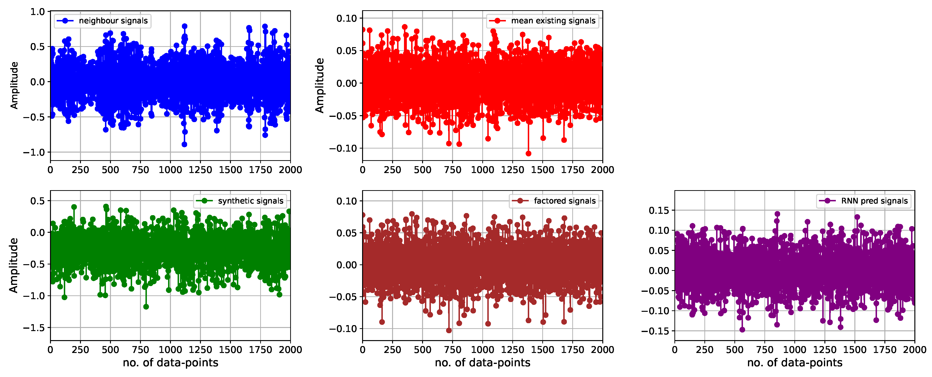
Every data point of the mean existing signals is multiplied with randomly generated factors between 0.7 and 1.1. The range takes into account the amplitudes of the FFT plot for the mean existing signals. The factored signals are in the same range as that of the reference mean existing signals. As displayed in
Figure 3, it would be advantageous if the amplitudes of the non-peak signals were larger than the mean signals. This adjustment would allow for the incorporation of individual signal characteristics more effectively, resembling those observed in the corresponding reference signals.
2.5.3. RNN-Regressed Signals
Finally, missing signals are generated by training an RNN model for a regression task. RNNs excel at capturing sequential trends within data points by utilizing both the current input and the information from previous outputs to make predictions [
48]. This may further contribute to introducing meaningful variability to each data point. This variability enables each data point to have its own distinct identity while still aligning with the reference signals. It is important to note that these data points are not directly derived through factorization from the corresponding data points in the reference signals, as is the case with the factored signals.
Figure 3 shows plots of both the reference and generated signals. As can be observed, the synthetic signals are shifted more to the negative values.
The final set of signals is generated by initially substituting the values of the mean existing signals in place of the missing signals. Subsequently, the entire dataset, encompassing both the existing signals and the replaced missing signals, is employed as both the training and target dataset. Once the RNN model is trained, predictions are generated for the missing signals.
The neural network architecture comprises an input layer with 8192 neurons, a hidden layer with 10,000 neurons, and an output layer with 8192 neurons. The mean squared error is employed as the loss function, with a batch size of 32 and 100 epochs. The inclusion of a larger hidden layer is intended to maintain the amplitude between the mean of existing signals and the neighboring signals. The amplitude for the mean of existing signals is less than 250, whereas that of neighboring signals is around 500. Consequently, the generated signal exhibits an amplitude of 227, within the stated range, and the achieved loss is 0.0556.
In this scenario, the accuracy of the model need not be excessively high for the generation of missing signals that are not identical to the input. Typically, zeros are assigned to missing data during the training of RNN models. However, for time series signals with distinct characteristics, assigning values such as the mean of existing signals is more reasonable. This approach allows the model to better capture the trends and peaks expected in the missing signal predictions.
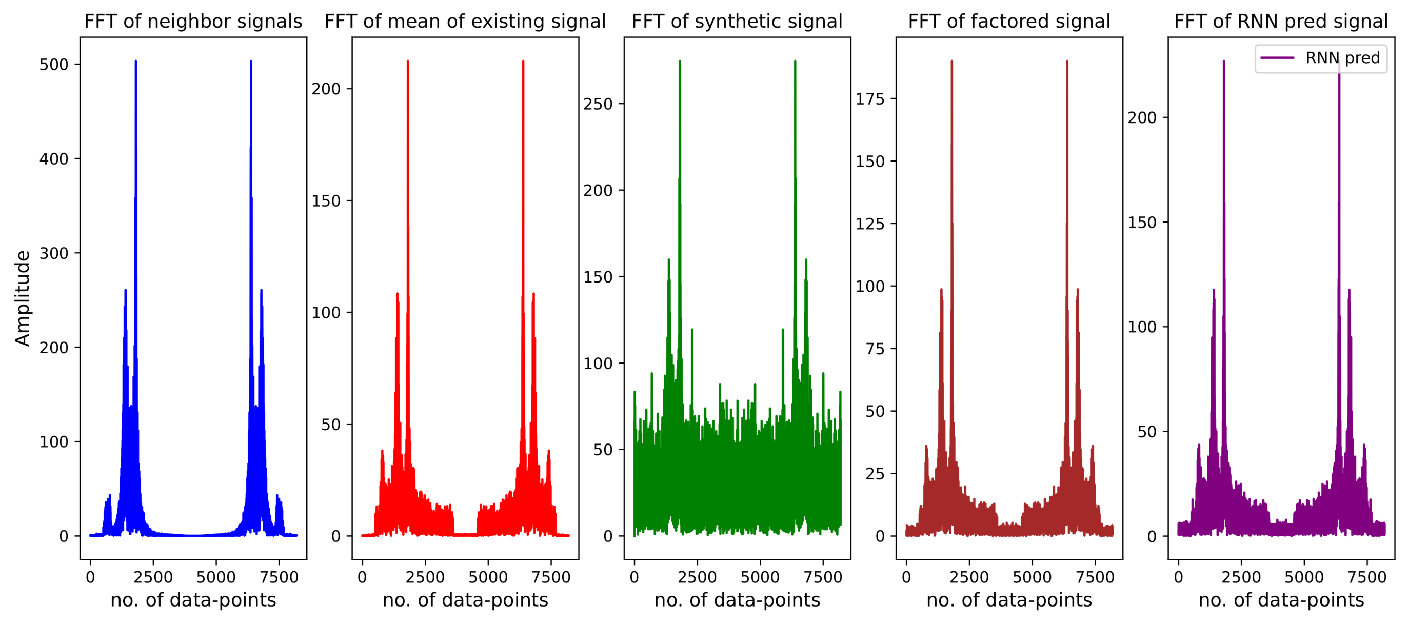
The FFT plots in
Figure 4 show that the synthetic signals’ trends, especially for the lower amplitudes near the peaks, are larger and not decaying, as opposed to the corresponding plots of the neighboring signals and the mean existing signals. For this reason, the approach of factoring the mean of existing signals was implemented. In terms of the trend, these signals perfectly matched the reference ones. However, as observed from the neighboring reference signal, the generated signals should also exhibit their trend to some extent.
The RNN-regressed signals now possess both required qualities: their values range between those of the individual signals (the neighboring signal in this case) and the mean existing signals. The trend is also similar, although not an exact match to that of the reference signals, fulfilling the necessary criteria.
In this study, therefore, the RNN-regressed signals are utilized in place of missing signals from the healthy condition of the given experimental building structure.
3. Feature Extraction and Selection
One of the crucial steps in machine learning is feature extraction, and, of course, feature selection. Features are the variables deemed to contain a significant amount of information from the given dataset. With these features, models can be trained and tested to make predictions. To effectively train models capable of capturing trends from signals of both healthy and damaged structural conditions, feature extraction is imperative.
In this study, time-domain, frequency-domain, and time–frequency-domain coefficients are employed for feature extraction. Specifically, PSD coefficients and WT coefficients are utilized for their effectiveness [
42,
49,
50].
3.1. Time-Domain Signals without Feature Extraction and with PCA
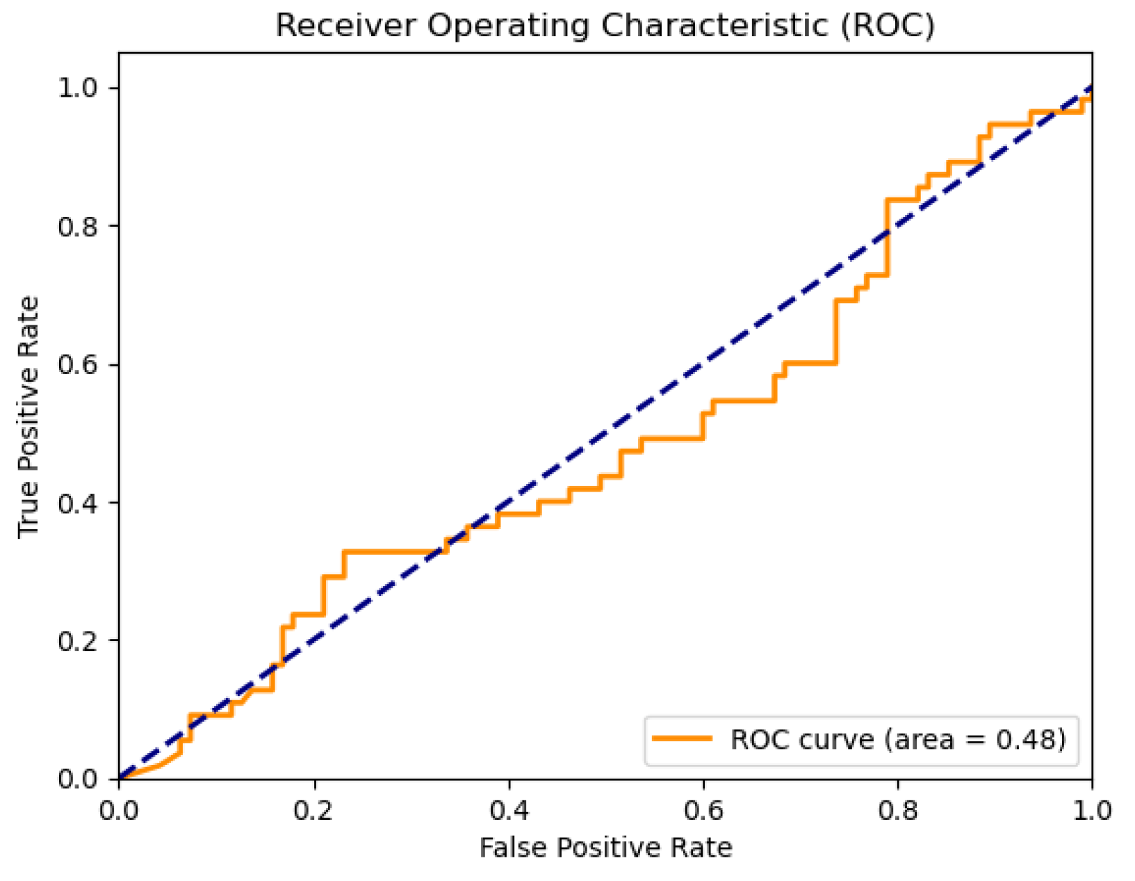
After the normalization of the dataset, the time series domain is utilized without further feature extraction. Accordingly, an NN model with an input layer consisting of 8192 neurons and a hidden layer containing 5000 neurons is trained. A learning rate of 0.002 is set, along with L1 and L2 regularizations of 0.001 and 0.0002, respectively. The model is trained for 500 epochs, resulting in a test loss of 13.55 and test accuracy of 0.451. The receiver operating characteristic (ROC) plot’s area under the curve (AUC) value of 0.5 indicates random prediction, further confirming the poor performance of the model. Additionally, the large number of neurons in both the input and output layers leads to a larger computational burden.
Following PCA preprocessing on the dataset, only the first 400 principal components are retained, explaining 98.8% of the variance. Consequently, the input and hidden layers of the model are significantly reduced to 400 and 250 neurons, respectively. While keeping other parameters constant, such as the learning rate and regularization values, and increasing the number of epochs to 1000, the model’s training loss decreases to 1.69 and the test accuracy improves to 0.547. From the above model, it is evident that, despite the improvements in the training loss and test accuracy, the AUC performance remains poor.
To further investigate, the number of PCA components is reduced to 150, and the ROC AUC result is observed as 0.48 on an unseen prediction dataset consisting of 150 signals. Although the input layer is then reduced to 150 and the hidden layer to 80, and the test loss is recorded as 0.848 and test accuracy as 0.783, the AUC displayed in
Figure 5 still depicts the poor performance of the trained model. Other feature extraction approaches therefore need to be implemented.
3.2. Frequency-Domain Features
Time series signals are transformed into the frequency domain using the fast Fourier transform. As vibration-based signals, like the acceleration signals used in this study, are well elucidated in the frequency domain, leveraging these coefficients as features is justified. PSDs are particularly valuable in illustrating the distribution of frequencies, including the natural frequencies that convey information regarding characteristic changes in structures—which we call damage [
40,
51]. Consequently, we utilize the peak amplitude, peak frequency, crest factor, skewness, and kurtosis of each considered signal segment from the respective PSD plots. The sensitivity analyses conducted below are therefore based on these coefficients.
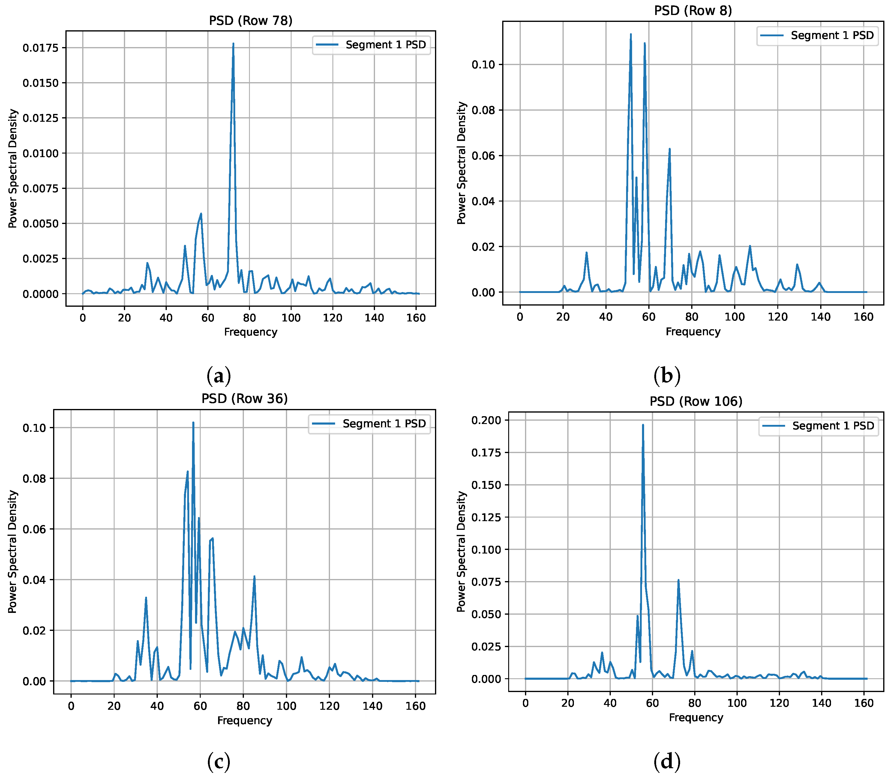
The PSD plots for the sample signals from all four conditions—undamaged (row 78), with EOFs (row 8), damaged (row 36), and EOFs with damage (row 106), respectively—are given in
Figure 6, after the RNN-regressed signals are used to replace the missing signals and data normalization is carried out. The PA and PF coefficients of all three states other than the healthy condition are close to each other, with PA 0.11, 0.1, 0.2 and PF 51.61, 56.77, 55.48, respectively, whereas the undamaged condition signal has PA 0.046 and PF 72.26. Such a shift in the natural frequency of the signal in subplot B is caused by the increase in mass on the first floor to represent operational effects, which seem even to exceed that of the damage represented by a 10 mm bumper gap, as shown in subplot C. The CF values for the damaged and EOFs with damage categories also are similar, at 2.99 and 2.98, respectively. All these effects show that the EOFs’ effects weigh the same or more than that of the damaged status. All 680 such signals are thus used throughout the work that follows.
Sensitivity analyses of the segment length and overlapping percentage, including the effects of PCA, are covered using PSD coefficients, and then the best approach for each sensitivity analysis is kept in the remaining part of this study.
As can be seen in
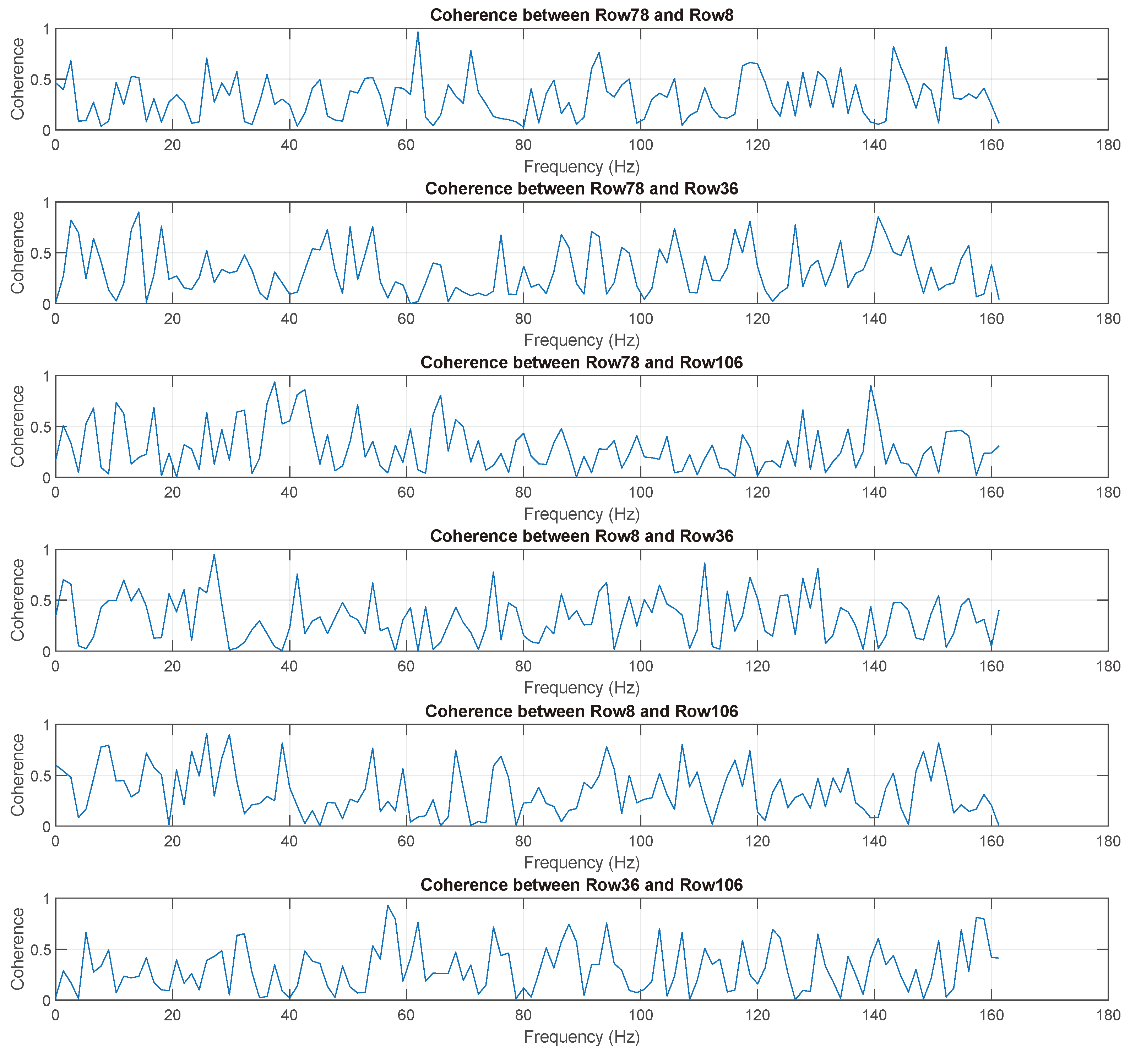
Figure 7, the signals were segmented into 250 segment lengths and 50% overlapping was used with a Hamming window to plot the coherence among four randomly chosen signals from different exposure states using Matlab R2019b. Coherence plots for the randomly selected signals from different conditions provide insights into the frequency ranges in which the coherence becomes considerable. As the first 20 Hz frequency range mainly corresponds to the rigid body modes of the structure and the excitation was random between 20 Hz and 150 Hz [
26], the coherence plot is inspected only to this band. The amplitudes for the PSD plots in
Figure 6 also reflect this reality.
Accordingly, high coherence between the undamaged signal (row 78) and the signal with EOFs (row 8) is observed only at a few frequencies, at 25.8 Hz, 61.9 Hz, 71 Hz, 92.9 Hz, 143.2 Hz, and 152.3 Hz, with the highest coherence at 61.9Hz, and the magnitude is 0.96. No considerable bandwidth with high coherence exists, which is an indication that the EOFs have a strong influence on the row 8 signal. See the topmost plot in
Figure 7.
For the next subplot, in which the undamaged signal is paired with the damaged one (row 36), low coherence is observed in multiple bandwidths. These are between 20 and 46.4 Hz, 55.4 and 90.3 Hz, 92.9 and 104.5 Hz, 107.1 and 117.4 Hz, 120 and 125.2 Hz, 127.7 and 139.4 Hz, and finally between 141.9 and 149.7 Hz. These bands exhibit coherence as low as zero and as high as only 0.6, not far from the moderate value considered here, which is 0.5 coherence.
The third subplot displays relatively low coherence between the undamaged signal and the signal exposed to both damage and EOFs (row 106). Except at four frequencies, the whole bandwidth is covered with low coherence. Although the signals on row 36 and row 106 face the same damage level (20 mm bumper gap), the EOFs imposed on the row 106 signal indicate no significant influence and therefore return a smaller number of frequencies with high coherence to the undamaged signal.
The remaining three subplots display the coherence among the three signals, excluding the undamaged one. Although, because of the above observation, bandwidths with higher coherence are expected, the reality is different. Even the frequencies that correspond to high coherence do not match across the three subplots. Therefore, although the coherence plot provides a very good understanding of the given dataset and the corresponding conditions, and its candidacy as an input for feature extraction is undeniable, it remains difficult to extract meaningful features across the whole signal based on this analysis.
3.3. Overlapping Percentage
Signals may be segmented for various reasons. Segmented signals offer the advantage of easily capturing the details of a given signal, are more manageable, and can be used as a strategy to handle non-stationary signals. In this study, even though sample time series plots and statistical measures such as the mean and variance show no considerable changes, and thus the signals could be considered stationary, segmentation is also implemented as a tool to address the non-stationarity of the signals. Moreover, segmentation is employed as a strategy to extract time-resolution-dependent information from the PSD plots, since this FFT lacks this.
Segmentation by itself, however, introduces information leakage at the edges of segments when one tries to restore the original signal. This shortcoming is minimized using windowing. By implementing windowing, we aim to ensure uniformity in the starting and ending points of signal segments when the FFT process is underway. This approach is designed to yield a refined FFT result. As a result, the dominance of specific frequency bands around a primary signal in comparison to other signals can be alleviated. Various windowing techniques exist to reduce leakage effects during the segmentation process. The Hamming window has a very good trade-off between the main lobe width and side lobe levels. For this task, therefore, we use the Hamming window.
where
and
N is the number of data fed to the FFT. Equation (
3) is the formula for the Hamming window. It is quite close to the Hann window but has a very good trade-off between the main and side lobe widths.
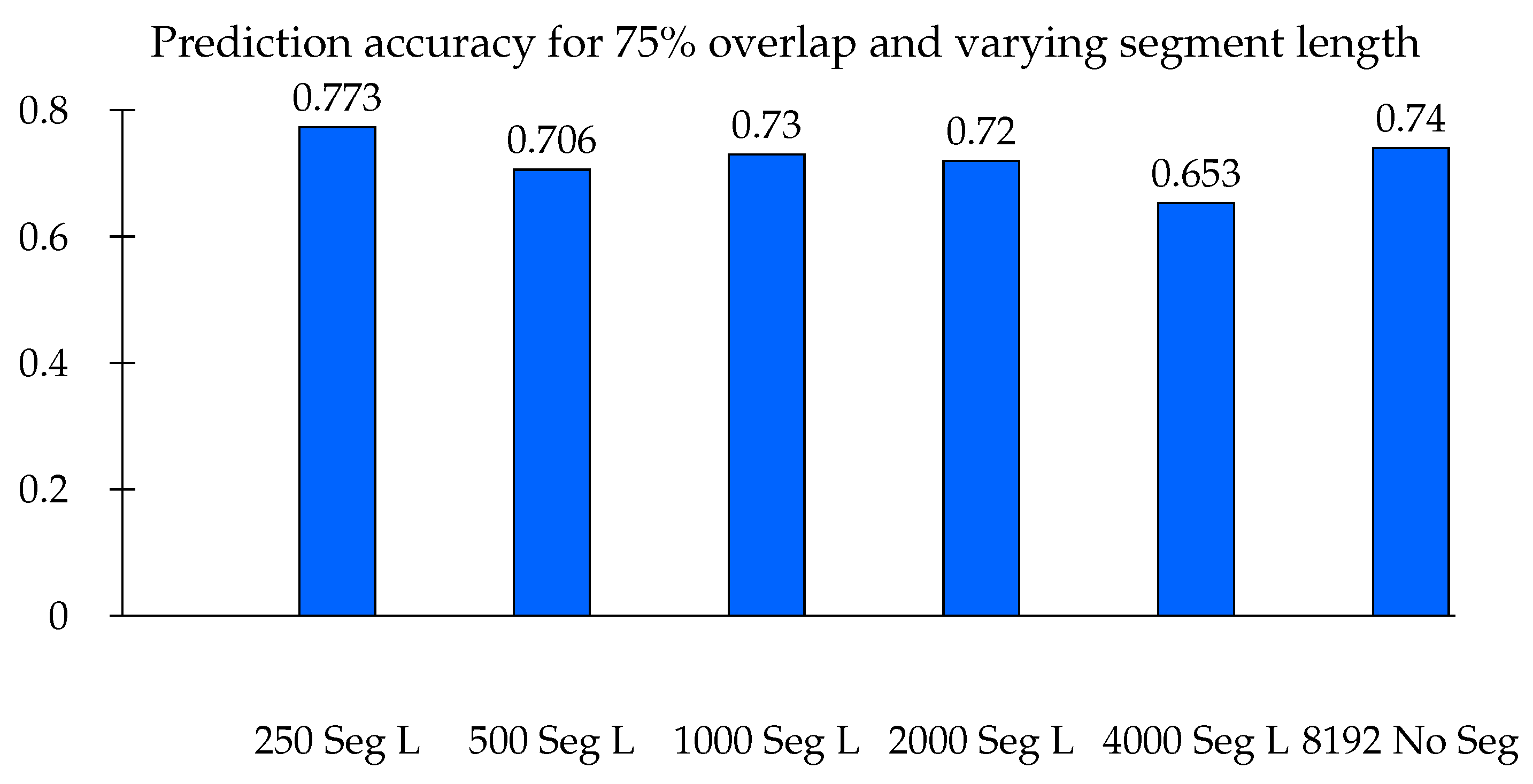
Unlike Hann, the Hamming window’s ends do not touch the zero-value mark. However, they are still quite similar to each other. To start with, a segment length of 250 data points is chosen. The performance of three segment length overlapping percentages is compared. They are commonly used and advised overlap percentages, 50%, 75%, and 90%. The NN models have a learning rate of 0.002, dropout rate of 0.1, loss patience for early stoppage of 5, and regularization factors L1 0.001, L2 0.0001. Based on the accuracy of the trained NN model, the 75% overlap shows better performance, with 77.3% accuracy.
The neural network models were tested with both one and two hidden layers. For this task, a single hidden layer proved to be sufficient and yielded better results compared to the two-layer architecture. The number of neurons in a particular hidden layer is another hyperparameter that demands careful consideration. In research, it is not set to a specific number; its optimality depends on factors such as the complexity of the problem, the data quality, and the number of neurons in both the input and output layers.
It might be generally said that a higher number of neurons in the hidden layer improves the performance of the model. This, however, does not work indefinitely and it is also at the cost of time and computational memory consumption [
52]. In this regard, several neurons in the hidden layer might be given between
and
of the total neurons in both the input and output layers. In this work, for general comparison purposes, the number of neurons in the hidden layer is taken to be half the sum of that of both the input and output layers.
The performance of the overlapping percentage is summarized in
Table 4. The prediction accuracy for 75% overlapping showed slightly better performance, at 77.3%; with PCA as a dimensionality reduction method, 50% overlapping has slightly more accuracy, at 68.6%, followed by 65.3% for the 75% overlap. Although a 74% prediction in the 90% overlap is not significantly lower accuracy, the high dimensionality of the features with the increased overlap percentage strongly affects the task. In this case, 1590 features are used for the 90% overlap, while 645 and 320 features are used for the 75% and 50% overlaps, respectively. The performance with PCA here is lower as compared to the use of the original features. Except for the RNN models used below, where the model training takes too much time, PCA is not used for the neural network models.
3.4. Segment Length
Now, the segment length of 250 data points is considered the smallest segment to start with. The next segment length results from the doubling of the preceding one. With this, five segments have been used to generate PSD features and train the NN models. Following the above result, note that the 75% overlap is used. Additionally, the original signal in its unsegmented form (with no segmentation, there is no need for windowing) is also included.
The neural network models’ accuracy in prediction using the PSD coefficients generated from different segment lengths with Hamming windowing applied is shown in
Figure 8. A total of six NN models were trained. As the same overlapping percentage was used across all six models, the numbers of features correspondingly decreased from the 250 segment length to the unsegmented original signal with 645, 310, 145, 65, 25, and 5 features, respectively. As can be seen in the same plot, the highest prediction accuracy is recorded for the 250 segment width.
3.5. Effect of PCA
Regarding
Table 4 above, the dimensionality is much reduced for the 50% overlap, from 320 to 70 features, with 99.7% of the variance in the original features explained; for the 75% overlap, it is reduced from 645 to 130 features, with the same 99.7% variance explained; and for the 90% overlap, it is reduced from 1590 to 150 features, with 95.5% variance explained. The use PCA reduced the dimensions of the features to be trained and the corresponding prediction results were of course smaller than those of the full-scale features. For this reason, we chose to use the original features except for the RNN models below.
Figure 9 shows the cumulative variance percentage explained with the corresponding number of PCA coefficients. The plot is specifically for the 75% overlapping case in association with
Table 4 above. With 130 PCA-transformed features, therefore, 99.7% of the variance in the original features is explained, thereby reducing 645 features to only 130.
From the above sensitivity analyses, which are based on the frequency coefficients and neural network models, the 75% segment overlap and the 250 data point segment width with no PCA reduction showed the best performance from their respective categories.
3.6. Wavelet Coefficients
The wavelet transform usually has an advantage over the Fourier transform in that the former can capture coefficients using high time and frequency resolutions, while the latter operates fully within the frequency domain. This enables WT coefficients to capture both low-frequency content that requires a high frequency resolution and high-frequency content that requires a high time resolution [
53].
The Daubechies wavelets, belonging to the family of orthogonal wavelets, are distinguished by their maximal number of vanishing moments. These wavelets consist of scaling functions, also known as father wavelets, employed to represent the coarsest level of approximation in multi-resolution analysis. They yield approximation coefficients (CA) capturing low-frequency content. Additionally, there are shifting functions, or mother wavelets, which provide detail coefficients (CD), representing high-frequency content. In this feature extraction task, the db4 (which has four wavelet and scaling coefficients) wavelets are specifically chosen. The wavelet is applied to all available signals with varying scaling.
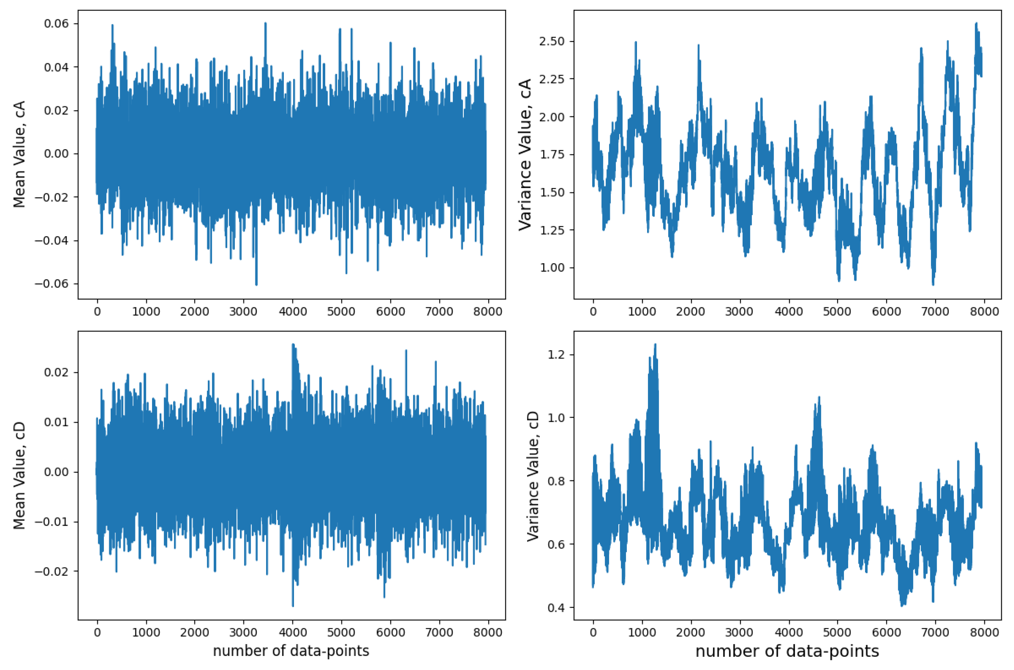
The mean and variance of each coefficient category are taken into account as extracted features. Given the observable differences among the data points of the coefficients, a second round of data normalization is implemented. A comparison is then conducted among multiple NN models using the aforementioned coefficients with various combinations.
CA and CD coefficients were used both separately and together while training the dataset. The power and energy of the coefficients were also computed to enhance the model’s quality.
Figure 10 shows the mean and variance of the sample signals from damaged conditions. Such coefficients are extracted to train damage-detecting models.
Other than the CA and CD coefficients, the energy coefficient, which is the square of the sum of the CA and CD coefficients, and the power coefficient, which is the energy quotient for the product of several features, and the sampling rate are also used. With these coefficients, there is a significant reduction in the feature dimension.
The separate coefficients of the CA and CD categories each have 516 features, with both categories containing 1032 features. In the last three model categories containing power and energy, each has only two features. Seven neural network models trained with combinations of wavelet coefficients have relatively closer performance, as can be seen in
Figure 11. The power and energy coefficients derived from the detailed coefficients scored 76%, closely followed by the model trained with the normalized CA and CD coefficients, with 74.6% prediction accuracy. A model with power and energy coefficients derived from both CA and CD also scored 73% accuracy. In this regard, it may be possible to use any of the top-performing coefficients or their combinations. The prediction accuracy for all models in this subsection and in the entire work is that obtained on unseen datasets.
3.7. Most Damage-Sensitive Segment (MDSS) Extraction Approach
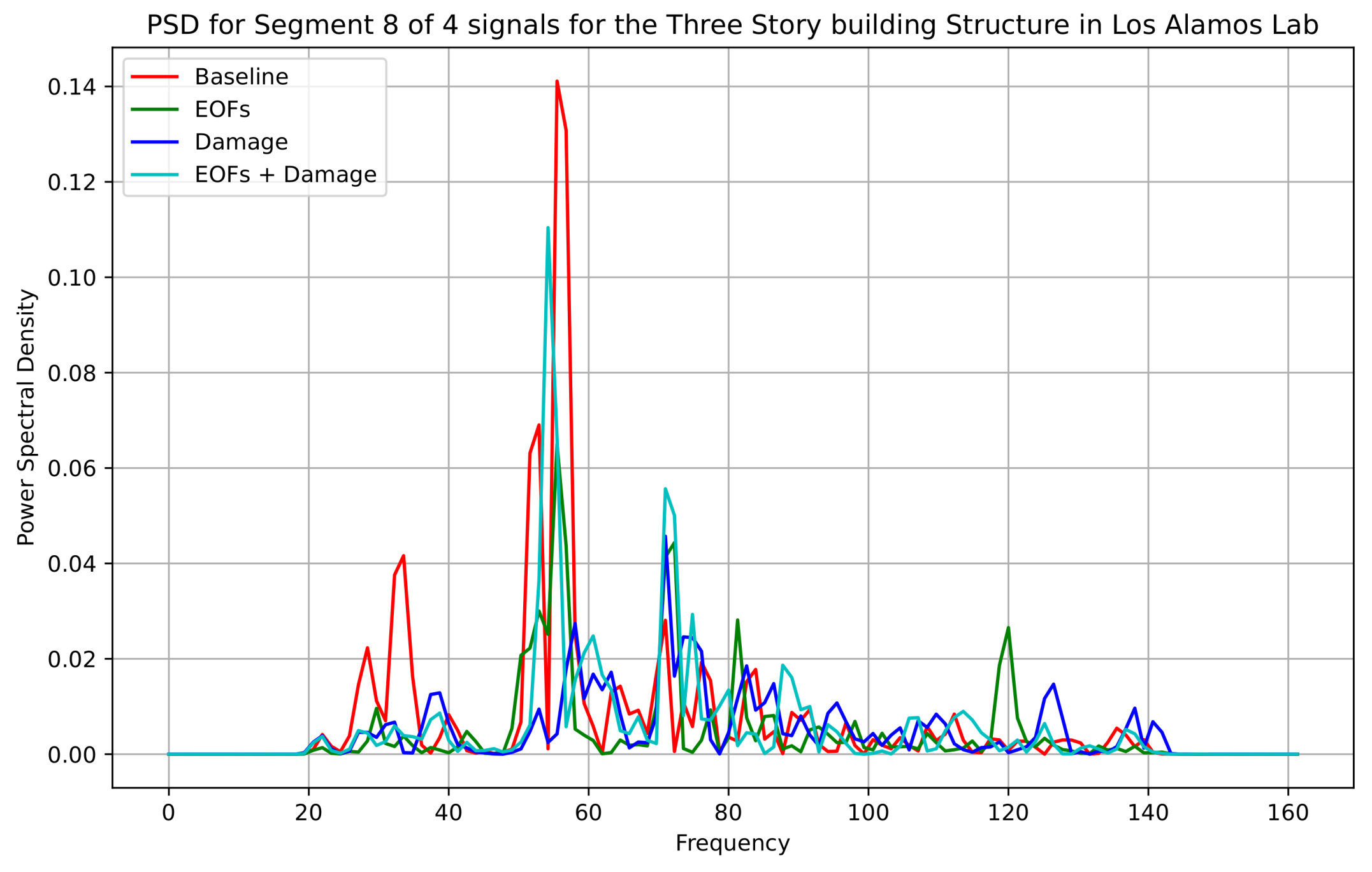
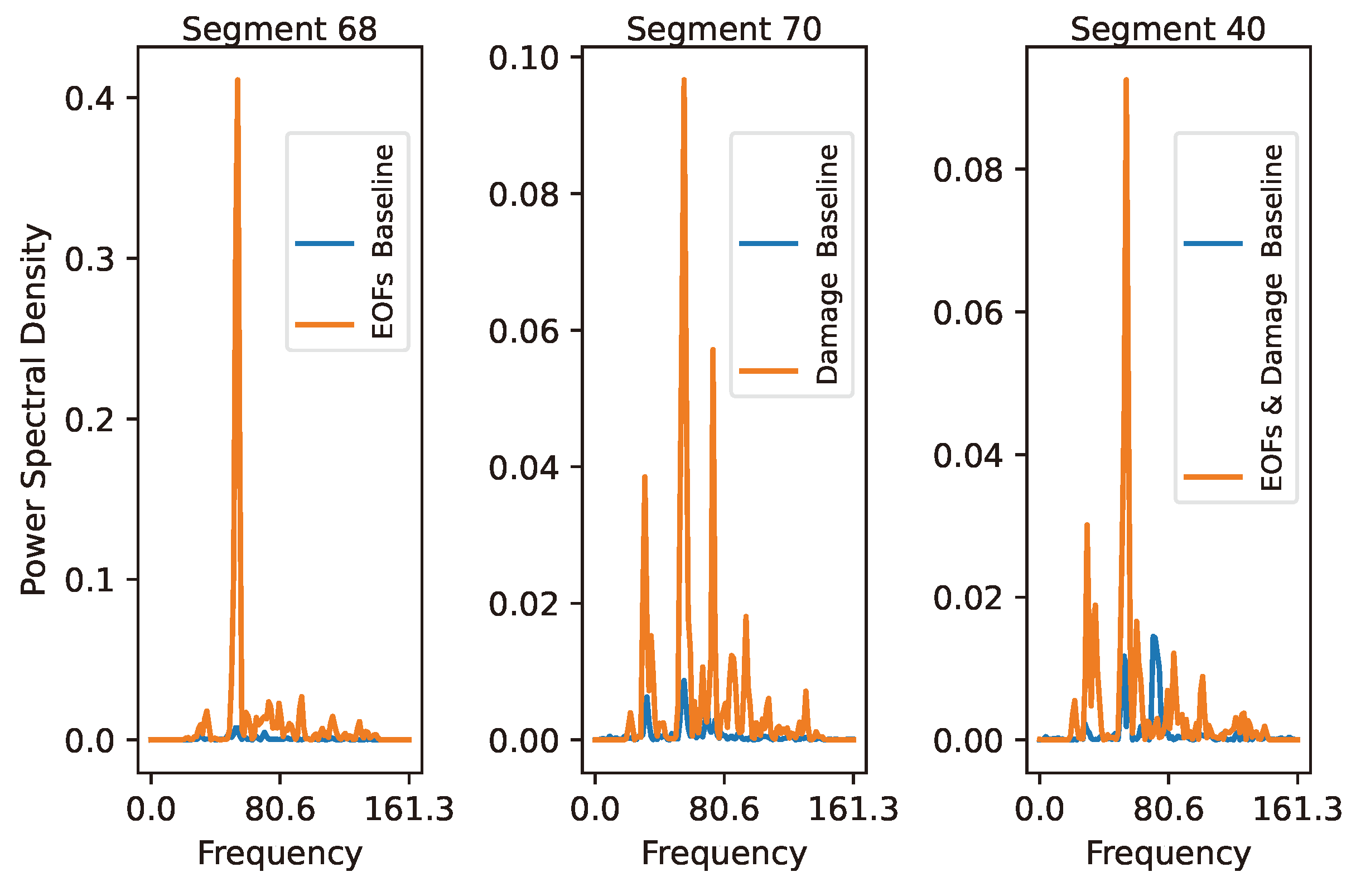
The nature of the signals was studied at the segment level to determine whether there were noticeable patterns among the signals of different categories. From a 250 window length and 75% overlap, the eighth segments of the 75th, 15th, 35th, and 105th signals were randomly selected to correspond to the undamaged, with EOFs, damaged, and EOFs plus damaged conditions.
Therefore,
Figure 12 was plotted based on the maximum difference in the respective defined coefficients among a randomly chosen baseline (undamaged state) signal and all dataset signals. Accordingly, it was observed that the peak amplitude, crest factor, skewness, and other coefficients of the signals from the damaged condition exhibited relatively smaller values compared to the undamaged signals with EOFs. A considerable pattern was also observable among the four conditions of the signal segments as, generally, segments in the undamaged condition scored the largest coefficient values, followed by the EOFs with damage condition, the EOFs condition, and, finally, the damaged condition.
This is evident in certain segments of each signal. Most importantly, this insight leads to a segment-based feature extraction technique such that each signal returns its characteristics. Thus, extracting such segments may assist machine learning models in distinguishing a damaged state from those with EOFs and undamaged states.
Based on this insight, a procedure is developed to extract such features at a segment level and use them to train damage-detecting neural networks. A maximum change detection criterion is used to deal with the different conditions of the signals, including the EOFs.
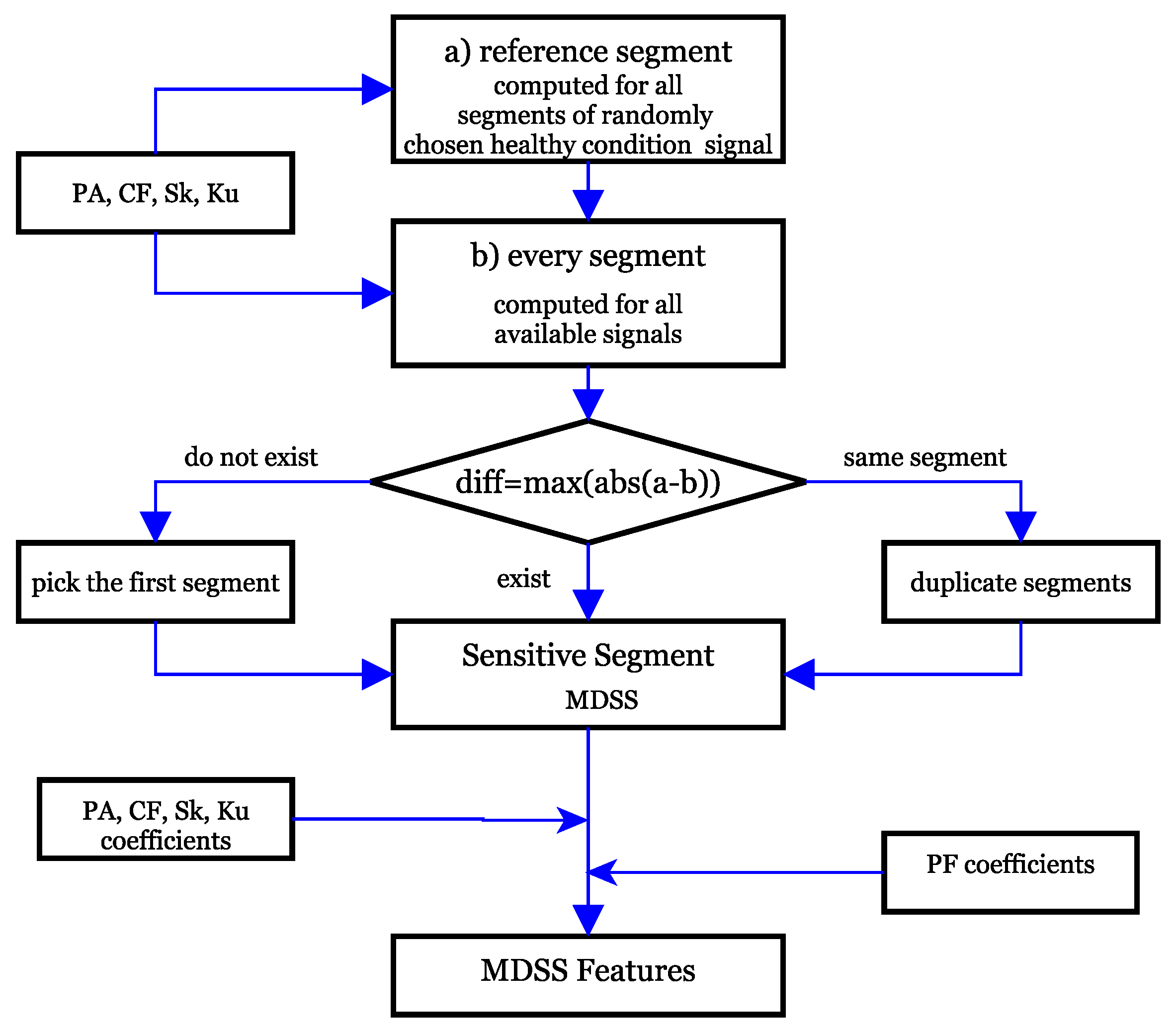
MDSS selection returns the most sensitive segment of each signal experiencing the maximum difference from the baseline signal for the considered coefficient. Each signal is therefore represented with several signal segments, each corresponding to a specific type of coefficient. The procedure is summarized as follows. First, a random signal from a healthy state is chosen. After it is segmented with a segment length of 250 data points and 75% overlap, their PA, PF, CF, Sk, and Ku coefficients are computed. These segments thus serve as references for the next step.
In the next step, for each of the available signal and condition categories in the given dataset, each of the above coefficients except PF is taken and the difference in magnitude between the healthy state segment and the corresponding segment of every signal is computed. Thus, the segment with the maximum absolute value difference is chosen as the most sensitive segment for a specific coefficient from a specific signal. The same is applied for the remaining coefficients.
In this way, there are four sensitive segments corresponding to the stated four coefficients for each signal. For each sensitive segment, all four coefficients are computed. Therefore, there are 16 coefficients for a given signal. At this point, PF, which was excluded as a criterion due to its direct dependency on PA, is included as an output coefficient, making a total of 20 coefficients for each signal. The flow chart in
Figure 13 shows the feature extraction process using the developed MDSS approach.
The same is applied for each of the 680 signals. At this point, the difference between the coefficients of the healthy state segments and all signals is computed. A segment that returns the maximum absolute value difference between the respective coefficients of corresponding signal segments is thus identified. Accordingly, each signal will have four MDSS segments. A segment may be the MDSS for more than one coefficient. In such a case, the segment is reused, as well as the coefficients. On the other hand, there may not be an MDSS if all corresponding segment differences for a coefficient result in the same value. In such a case, a segment is randomly chosen as the MDSS for the same specific coefficient.
Signal 78 from the healthy state was randomly chosen as a reference signal for the MDSS feature extraction. The 250 data point length and 75% overlapping produced 129 segments per signal. Then, five PSD coefficients, PA, PF, CF, Sk, and Ku, were computed for all 129 segments of signal 78.
In
Table 5, the MDSS chosen based on the procedure stated above for three signals from the three conditions are displayed. The numbers represent specific signal segments out of all available 129 segments for a specific signal. As can be seen, for the first and third signals, a segment was the MDSS for more than one coefficient. On the other hand, for the second signal, there were four distinct MDSS segments for each coefficient. The indices of the segments from healthy state 78 were the same as the corresponding displayed segments.
The PSD plots of the MDSS for the PA coefficient in
Figure 14 show the amplitude and frequency distribution of each MDSS and its corresponding segment from the healthy state signal 78. Although each segment is chosen as the MDSS for each coefficient, all five coefficients, including PF, are computed from each MDSS segment. This results in a total of 20 features for each signal. This highly reduces the dimensionality, even compared to PCA, which reduced a number of features to 70 features only. The PCA-treated features resulted in ML models with slightly reduced accuracy.
With this approach, a binary classification NN model was trained. The input layer had 20 neurons and the hidden layer had 14. Its training dataset imbalance was then handled using SMOTE oversampling with 6 k-neighbors. This treatment increased the test dataset from 424 to only 426, and it was less affected by SMOTE. The corresponding test loss and test accuracy given a 0.1 drop were 0.949 and 0.651, respectively. With the rest of the hyperparameters kept the same as in the other models above, its prediction accuracy showed an improvement compared to the other models, with 81.3% accuracy on the unseen datasets. The corresponding improved precision and recall scores were 0.755 and 0.72, respectively.
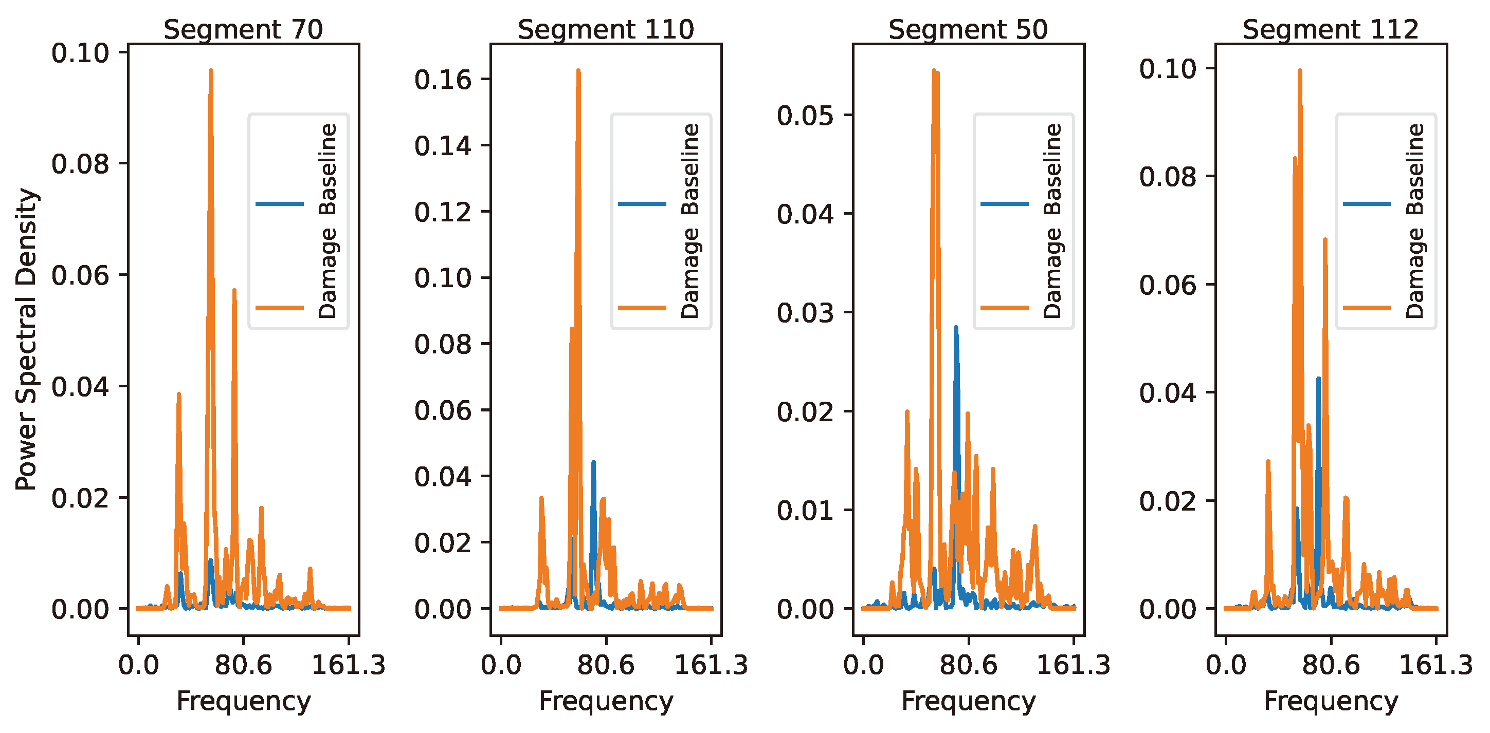
Four MDSS segments for the 35th signal, with results in all 20 features for the same signal, are plotted in
Figure 15, each with its respective segment from the undamaged condition of the 78th signal.
As the MDSS is deployed to a segment (segments are treated as points) rather than corresponding specific points on the same segment, shorter segment lengths or larger overlap percentages positively contribute to a more detailed frequency content examination (higher time resolution), thereby returning improved models, while negatively contributing to the computational burden. A trade-off is therefore required when working with big data.
MDSS is a technique to be used in an attempt to capture potential patterns that correspond to each coefficient type of interest at the segment level. It assumes that a change observed in a coefficient that is chosen based on domain knowledge potentially captures both damage-based and EOF-based changes, and it can readily be applied to any structure and diagnosis problem.
4. Damage Detection ML Models
EOFs can also be addressed with machine learning models. For this reason, multiple models based on different training features were developed and tested, and damage predictions on an unseen dataset were made using these models. In this section, the procedure followed for the training of the models and the outputs for damage detection, localization, and severity are presented.
4.1. Dataset Splitting and Unbalanced Dataset Handling
Out of the 680-signal dataset, 150 signals are reserved to measure the accuracy of the predictions made with these trained and fine-tuned models. The remaining 530 signals are used to train and test the damage detection machine learning models. Through a targeted random sampling approach, the 150 signals are selected from the main dataset.
The targeted random sampling approach followed here selects 150 signals randomly such that the remaining dataset has the same number of damaged and undamaged labels. This means that the dataset used to train and test the models is balanced. Therefore, the strategy to select signals from the undamaged target and the damaged target remains random. Accordingly, 95 signals from the undamaged state of the building structure and 55 signals from the damaged state of the building structure are sampled for prediction purposes as unseen datasets. The remaining 530 signals thus have an equal number of signals with both undamaged and damaged labels, i.e., 265 signals each.
However, in the data splitting stage, the random splitting strategy introduces a data imbalance, especially on the training dataset. An imbalanced dataset occurs when the number of elements in each target class varies significantly. This imbalance can have a profound impact on the quality of the model, and, of course, predictions made with such data may not be reliable. To address this issue, targeted sampling and the Synthetic Minority Oversampling Technique (SMOTE) are implemented.
In this approach, 20% of the dataset is randomly split as a testing dataset and the remaining 80% is used as a training dataset. However, the imbalanced training dataset needs to be treated with SMOTE. As per this method, signals with labeling minorities are synthetically generated using the neighborhood values. It works as an oversample. The number of neighbors used is tuned to avoid overfitting and underfitting as well. In this work, however, the default value, 6 neighborhoods, is used to ensure a fair comparison among the different models.
Moreover, random undersampling was also applied for SMOTE to solve the dataset imbalance problem by generating unavailable data through random sampling.
4.2. Neural Networks (NNs)
Acceleration signals, including their labeling, were collected based on four conditions and their combinations. Supervised machine learning models were then trained here. Both the FFT and WT coefficients of various combinations were used to train multiple NN models. Two RNN models were also trained with these coefficients. As the RNN training process here was too slow, PCA was applied to reduce the dimensionality. However, the limited availability of prediction datasets greatly affected the accuracy, especially that of the WT-based model.
The NN model is structured with an input layer of extracted and selected features, followed by one hidden layer with neurons equal to half the total of both the input and output layers. The output layer has several neurons based on the type of model.
Both binary and multiclass classification models are trained. The binary classification model categorizes the signal condition as damaged or undamaged and thus requires only one neuron in its output layer. ReLU activation functions are used in the input and hidden layers, while the output layer is activated with Sigmoid.
During the forward feed, weights and biases are randomly assigned. The backpropagation process updates these coefficients based on the binary cross-entropy loss function. The loss function calculates the difference between the true and predicted labels and minimizes this difference using the Adam optimizer. This process is repeated for 1000 epochs.
The multiclass classification model has the same structure as the binary model, except that the output layer has neurons with sizes equal to the number of classes. In this case, there are five classes. Therefore, the activation function for the output layer is softmax, and the loss function is sparse cross-entropy. Hyperparameters such as the learning rate, dropout, L1 and L2 regularization, early stopping, and loss of patience are more or less the same. Dropout and regularization were applied to reduce the model’s memorizing tendency and thus enhance the generalization. This, of course, lowers the test accuracy of the model. The evaluation is therefore conducted using both the test dataset and a new dataset, while making predictions on the same model.
Simple RNN models with PCA-transformed coefficients are also trained: one with FFT coefficients and another with WT coefficients. Due to the limited size of the prediction dataset, only 90% of the variance was explained when PCA was applied to the FFT features, and 77% of the variance was explained when PCA was applied to WT. Therefore, the models were trained excessively, resulting in reduced feature sizes due to the limited prediction datasets. Accordingly, the prediction accuracy for the FFT-based RNN model is 64% and that of the WT-based is 71.3%. The WT-based RNN may obtain much better accuracy as it was trained for several features, i.e., more than 300, which resulted in variance explained of more than 95%.
4.3. Threshold Setting
Binary classification models require a threshold for prediction as their outputs provide a percentage probability of being classified as label 0 or label 1. There are percentage-based thresholds like the 95th percentile. Youndin’s J value is also another approach that utilizes sensitivity and specificity.
Equation (
4) shows how the J value is computed. TP represents true positive, TN represents true negative, and FP represents false positive predictions.
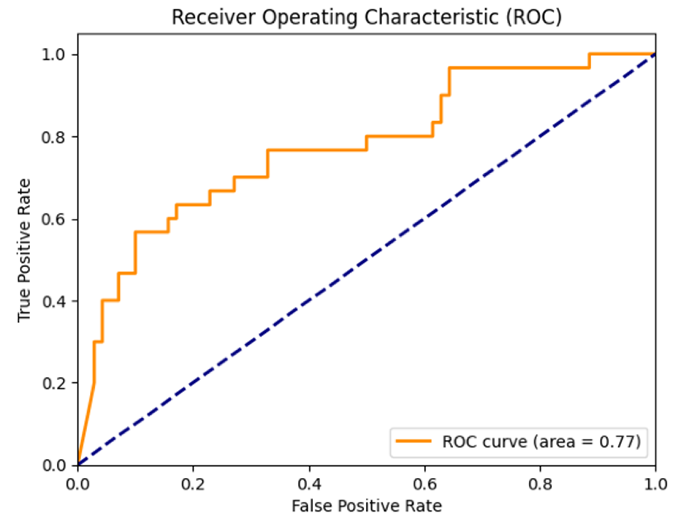
The third one is the receiver operating characteristic (ROC), which is associated with the maximum area under the curve. The ROC curve primarily plots the true positive rate against the false positive rate for threshold values ranging from zero to one. Models with ROC plots approaching the left vertical and top horizontal lines exhibit high accuracy, while those aligned with a broken straight line suggest near-random prediction accuracy [
34].
The performance of the 95th percentile is low. However, the results for Youden’s J value and the ROC are nearly the same. In this work, we choose the ROC threshold approach because it provides a more explainable output.
From the ROC plot in
Figure 16, thresholds with larger TP and smaller FP rates are preferable. The optimal threshold was automatically selected as 0.929.
4.4. Damage Detection
Binary classification and multiclass classification machine learning models are employed to detect damage. Signals from the undamaged condition of the structure are labeled as 0 (true negative), and those from the damaged condition are labeled as 1 (true positive). Since the prediction output is continuous, a threshold is applied to classify signals as damaged or undamaged. Damage detection is also performed using the multiclass classification model.
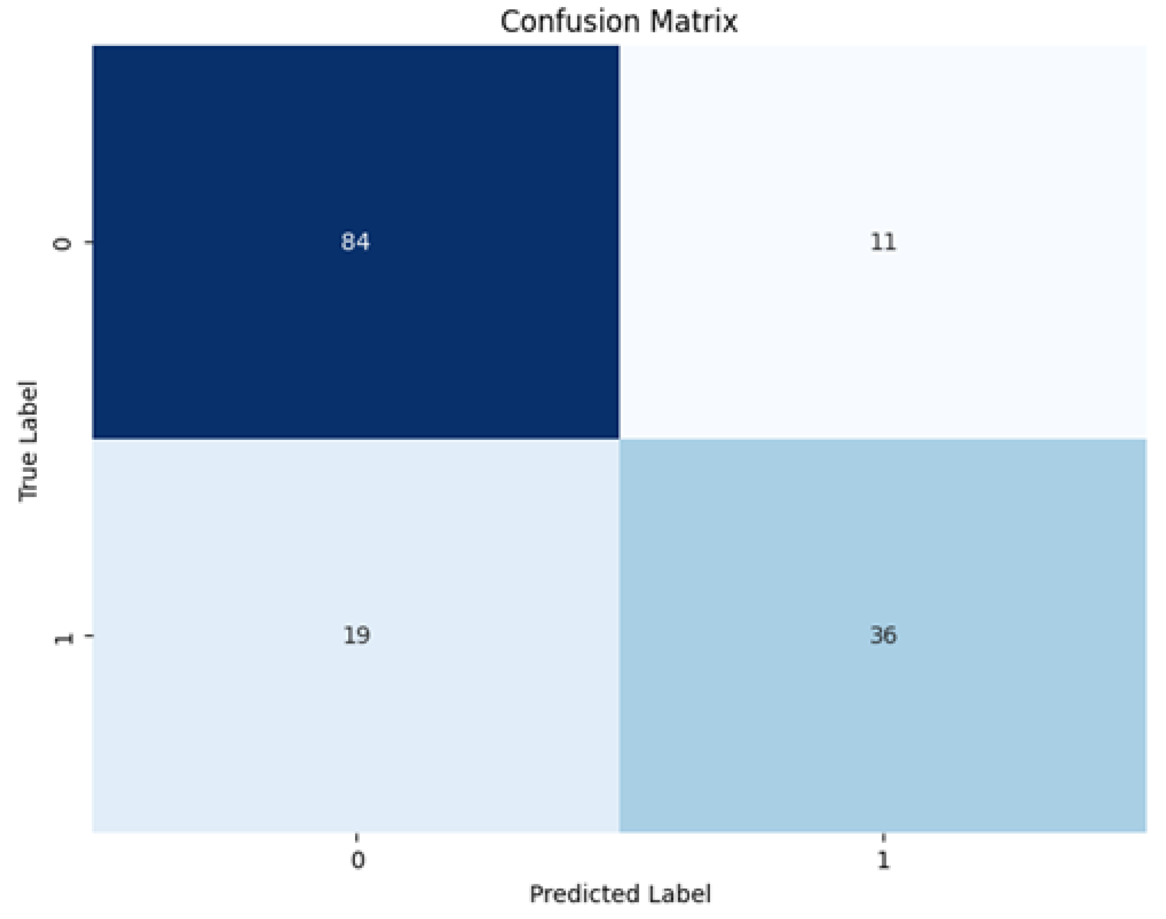
The confusion matrix for the binary classification model shown above in
Figure 17 is specifically that of the 250 data point, 75% overlap case with FFT coefficients used as training features. The prediction made on the unseen dataset resulted in 0.766 precision and 0.655 recall, with an F1-score of 0.706.
These models were trained considering three cases regarding the data imbalance in the training dataset: the unbalanced case, the SMOTE balanced case (oversampling), and the random undersampling balanced case. Binary classifications with the original unbalanced case performed best as compared to the other two, with 80% accuracy. Random undersampling also resulted in 75.3% accuracy, while the SMOTE approach’s performance was poor, at only 43%. SMOTE resulted in 10 additional samples and random undersampling resulted in a 10 sample reduction from the original training dataset size of 424.
where
represents the class assigned to the
i-th data point from 0 to 4,
n is the number of classes, and
is the
i-th data point probability.
With the multiclass classifications plotted as a and b on
Figure 18, binary classification predictions can be extracted. Two approaches were followed when the multiclass classification predictions were made. In the first one, the signal with the highest probability score determined the class, while, in the second one, a weighted average of all the classes is obtained via Equation (
5). Accordingly, the first option has 76% damage detection accuracy and the second option has 72% accuracy. With SMOTE applied, however, for option 1, 60% accuracy is obtained; for option 2, only 36% accuracy is recorded. With random undersampling, the multiclass classification models showed almost the same prediction accuracy of 70% and 69.3% for options 1 and 2, respectively.
In the unbalanced case with option 1, multiclass classification resulted in prediction accuracy of 76%, 95.3%, 86%, 82.6%, and 75.3%, respectively, from class 0 to class 4. The second option resulted in 74.6%, 92.6%, 83%, 82%, and 78%, respectively.
4.5. Damage Localization
Damage localization refers to predicting the position or area where damage has occurred. One approach to achieve this is to include the coordinates of the labels during training. This allows predictions using the same model to return not only damage instances but also their corresponding locations.
In this specific work, conducting in-depth damage localization was difficult given that only a single sensor was present on each story. It was thus infeasible to produce interpolation or extrapolation damage localization approaches. In addition, each floor had a square shape with a size of 30.5 cm and each column’s height was only 17.4 cm. As the model size was small, locating the damage position based on the respective floor sensor locations was considered appropriate. The acceleration sensors used in the data collection process had 1000 mV/g detection and fell within the point sensor category. The damage localization performed here was also specific to the location of each sensor, rather than the length or area.
Since the unseen dataset used to make predictions using the trained models was collected from the same structure, and the location of each signal was known during the data collection phase, the task here was to include the coordinates or floors where each signal’s sensor was located in the training models. This allowed the return of location outputs for the damaged conditions.
Accordingly, based on the damage detection approach in the above section, damage was located using both binary classification and multiclass classification models.
Table 6 summarizes the outputs. On the first and fourth signals, the multiclass predictions detected the damage and identified it as located in story 2. On the second and fifth signals, false predictions were made, including those for the associated locations.
4.6. Damage Severity
The severity level of the damage in the experimental setup was influenced by the bumper–suspension column gap, based on the considered setup and assumptions. Specifically, the larger the gap, the higher the nonlinearity introduced to the structure. Consequently, the severity of the damage was expected to be larger with a larger gap.
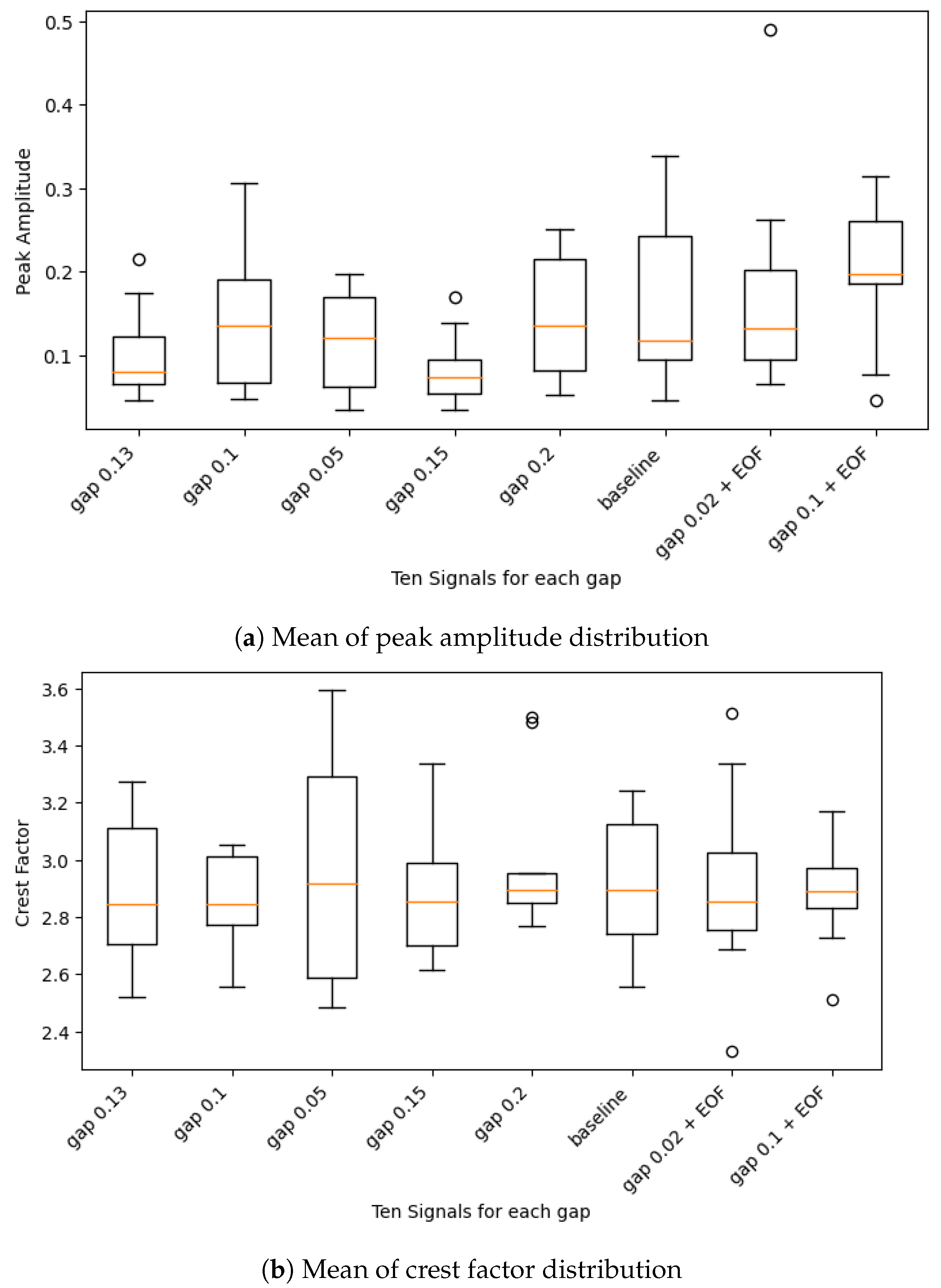
In this regard, therefore, the first task was to categorize the damage severity given the bumper gaps and corresponding signals collected. Eight signals were chosen, of which the first five had bumper gaps of 0.13, 0.1, 0.05, 0.15, and 0.2 mm, as well as a healthy baseline signal and two signals with EOFs and associated bumper gaps of 0.2 and 0.1 mm. The peak frequency, peak amplitude, crest factor, skewness, and kurtosis were extracted from their respective PSD computations for the 250 data point segment width and 75% overlap. The respective mean was then calculated and box plots of all eight signals for each coefficient were plotted to observe the distribution.
With the help of the peak amplitude and crest factor, the bumper gaps of 0.13 and 0.15 mm were grouped as their distributions had similarities, as can be seen in
Figure 19. Therefore, the severity categories were assigned values of 0 for undamaged, 1 for less damage with a bumper gap of 0.05 mm, 2 for medium damage with a bumper gap of 0.1mm, 3 for severe damage with bumper gaps of 0.13 and 0.15 mm, and 4 for very severe damage with bumper gaps of 0.2 mm. The severity extents may not perfectly align with the reality. They were implemented only to show the categorical differences in the damage.
As can be seen in
Table 6 above, the damage severity classifications were made using both option 1 and option 2.
The accuracy results for each model can be extracted from the confusion matrices provided above in
Figure 18. Therefore, predictions with option 2 in the unbalanced case resulted in 76%, 95.3%, 86%, 82.6%, and 75.3% accuracy for classes 0, 1, 2, 3, and 4, respectively.
Generally, the unbalanced dataset predictions exhibited better accuracy, followed by undersampled models, while oversampled models showed poor performance. One potential reason for this was the large number of synthetic samples (more than two times the original training dataset), resulting in overfitted models and less generalization. This may also be because of the lesser dataset imbalance effect compared to the relatively larger synthetic dataset required with SMOTE.
Figure 20 shows that, for multiclass classification, both SMOTE and random undersampling resulted in a very different synthetic training dataset from the original unbalanced one. In the multiclass damage severity classifications, option 2 showed better performance than option 1. Furthermore, the smaller number of labeled samples for each bumper gap class contributed to the reduced performance of the SMOTE oversampling and random undersampling models, ultimately favoring the original unbalanced models.
5. Conclusions
Six hundred and eighty acceleration signals, each containing 8192 data points, collected from an experimental three-story 3D frame structure, were used for training, testing, and prediction to mainly detect damages. The effort was also extended to damage localization and severity assessment. The objective was to examine the performance of potential feature extraction approaches using data-driven ML models to detect damage from signals under different approaches. Proposing a potential technique that could be easily integrated into existing approaches was another objective.
Sensitivity analyses related to the segment length and overlapping percentage were carried out. The effect of dimensionality reduction via PCA also was part of this analysis.
Although the time-domain signals in both cases without feature extraction and with the implementation of PCA were applied, the AUCs of the ROC plots indicated highly random predictions, which was due to the poor quality of the models. Different combinations of the FFT and WT coefficients were also used to train both NN and RNN models. Moreover, the most damage-sensitive segment was introduced as a potential feature extraction approach.
Generally, different approaches were tested to replace missing data and the RNN-based regression approach resulted in better trends and amplitudes regarding the reference signals. Given 8192 data point signals, a 250 data point segment width was found effective. Given the Hamming window, 75% overlapping returned better models. PCA resulted in slightly less accurate models but was much more helpful in training RNN models, which require more time for the original features. The PSD coefficients PA, PF, CF, Sk, and Ku performed well in capturing information from the provided signals. The WT coefficients CA and CD, their energy, and the power coefficients returned models with slightly better accuracy than the PSD ones. The RNN models with WT coefficients indicated promising results given the limited availability of prediction datasets.
In the presence of signals exposed to multiple conditions, such as healthy, with EOFs, damaged, and with EOFs plus damage, the MDSS feature extraction procedure introduced here might be considered a potential technique. The approach outperformed all other feature extraction approaches and returned higher evaluation results for its corresponding machine learning model. It also greatly reduced the dimensionality as a signal with multiple segments was replaced with only a few of the most sensitive ones.
MDSS is a technique intended for deployment to capture potential patterns corresponding to each coefficient type of interest at the segment level. It essentially assumes that the change observed in a coefficient, chosen based on domain knowledge, can potentially capture changes related to both damage and EOFs. Consequently, it can be readily applied to any structural and diagnostic problem.
The damage detection and localization tasks were carried out using both binary and classification models with high accuracy. The damage severity assessment was carried out using classification models and the performance was very good. An unbalanced training dataset, a SMOTE-treated oversampled dataset, and a randomly undersampled dataset were used across the research. EOF effects could potentially be handled with NN models combined with corresponding feature extraction approaches.
Overall, 20 NN and RNN models were trained in this work using different features and their combinations.
Although it performed well for some binary classification models, with multiclass classification, SMOTE’s accuracy was the poorest among the studied approaches. This was potentially due to the much smaller number of signals from each severity class. The models’ accuracy could potentially surpass the recorded values mentioned here if there was a more extensive dataset available for the given experimental structure.
At this point, it is worth affirming that data-driven damage identification approaches present great potential in parallel to the size and quality of the dataset collected.


