Mathematical Formulation of Learning and Its Computational Complexity for Transformers’ Layers

Abstract

Transformers are the cornerstone of natural language processing and other much more complicated sequential modelling tasks. The training of these models, however, requires an enormous number of computations, with substantial economic and environmental impacts. An accurate estimation of the computational complexity of training would allow us to be aware in advance about the associated latency and energy consumption. Furthermore, with the advent of forward learning workloads, an estimation of the computational complexity of such neural network topologies is required in order to reliably compare backpropagation with these advanced learning procedures. This work describes a mathematical approach, independent from the deployment on a specific target, for estimating the complexity of training a transformer model. Hence, the equations used during backpropagation and forward learning algorithms are derived for each layer and their complexity is expressed in the form of MACCs and FLOPs. By adding all of these together accordingly to their embodiment into a complete topology and the learning rule taken into account, the total complexity of the desired transformer workload can be estimated.

1. Introduction

Transformers [1] have revolutionized the field of artificial intelligence (AI) by achieving unprecedented accuracy results over a broad variety of complex tasks, including natural language processing (NLP). Their performance, however, has been proven analytically to scale as a power law of the number of parameters of the model and the dataset size [2]. The inevitable consequences of such dependence are bigger model footprints, larger datasets and an increasing number of gradient descent iterations. The associated enormous number of computations and memory usage has critical economic, time and environmental impacts. As an example, the recent 175-billion-parameter GPT-3 [3] was trained for 300 billion tokens [4] with a total compute of ∼3640 petaflop/s-days. According to [5], this process emitted 502 tonnes of carbon dioxide and cost 1.8 million USD. Given the pivotal role computational complexity plays when training a transformer, it is fundamental to provide for it an accurate estimation. Moreover, a variety of alternative learning rules to backpropagation (BP) were recently proposed [6,7]. A precise complexity analysis would allow one to reliably compare these algorithms and quantifying the advantages that forward learning would bring with respect to BP. Ideally, the training complexity should be obtained by considering the single operations performed at the hardware level. This is not convenient for several reasons. First of all, it strictly depends upon the device used, whose knowledge is generally limited, restricting the generalizability of the prediction. Secondly, it is not trivial to obtain the low-level implementation of the training algorithm, which in turn depends on the AI runtime library being used. This paper is organized as follows: Section 2 describes the objectives of this work and its contributions; Section 3 cites the main related works in the known literature; Section 4 describes the notation and conventions adopted during the quantitative analysis of the learning algorithms; Section 5 reports the equations for learning with BP, PEPITA and MEMPEPITA and estimates their complexity for all transformer layers; Section 6 presents an example application of the results obtained, and Section 7 concludes the paper.

2. Key Contributions of This Work

In order to eliminate the dependence from the deployment device, this study introduces a mathematical approach that assesses the complexity of layers in a transformer topology solely based on mathematical expressions, rather than considering hardware operations. In this respect, the contributions brought by this paper can be summarized as follows:

•

A description of the equations implemented in BP, PEPITA and MEMPEPITA for all transformer layers;

•

A mathematical derivation of the weights’ and activations’ gradient with respect to the loss function;

•

Quantitative complexity analysis in terms of multiply and accumulate (MACCs) and floating point operations (FLOPs) of each layer for the forward pass, backward pass and weight updates.

3. Related Works

3.1. Automatic Differentiation

Currently, most AI algorithms are implemented in two major libraries: Tensorflow [8] and Pytorch [9]. Both of the aforementioned frameworks use reverse-mode automatic differentiation (i.e., autodiff) [10], namely BP. Autodiff creates a computational graph from the mathematical expression considered, where each node describes an operation and each edge a variable. During the forward pass, intermediate variables are populated, and each node is complemented with the derivatives of the outputs with respect to the inputs. During the backward pass, the gradient is obtained by leveraging the chain rule of differential calculus to compute partial derivatives of the objective with respect to the weights. The operations involved during training can be referred to as forward pass, backward pass (gradient of the loss with respect to the activations) and weight update (gradient of the loss with respect to the weights). In several works [3,11], the complexity of the backward pass and weight update is assumed to be $2\times$ that of the forward pass, which is true only in certain specific cases such as fully connected and convolutional layers. Regarding transformers, Ref. [2] empirically identified the relations between performance, training time, dataset size, number of parameters and amount of computation. Moreover, also in this case, the computational complexity of training was approximated to be $3\times$ that of a forward pass. To the best of the authors’ knowledge there is no work that has analytically described the computational complexity of the transformer topology.

3.2. Alternatives to Backpropagation

It is well known from theory that BP is not describing the learning process happening in the human brain [12,13]. There are four main aspects considered to be in contrast with neuro-biological observations. Firstly, during the backward pass, weights previously used during the forward pass are utilized to backpropagate the error. Considering that synapses in the brain are unidirectional, this characteristic of BP gives rise to the “weight symmetry” problem [14]. Secondly, when calculating the error gradient, the activities of the neurons computed during the forward pass are left unaffected. The freezing of the activities during the backward pass is incompatible with the behaving of feedback connections in neural circuits, through which the signal travels via modulating activities [15]. Thirdly, the modification of synaptic weights is influenced by downstream neurons and synapses, whereas synaptic learning in the brain is predominantly governed by localized signals that are contingent upon the activity of the interconnected neurons [16]. Lastly, in order to update the weights of the l-th layer, the forward pass has to end, and the backward pass has to arrive at such layer. This means that learning cannot happen in an online fashion, contrarily to biological evidence. Such problem is referred to as “update-locking” [17,18]. With the hope of creating a correspondence between deep learning and brain nature, a vast research field focused on finding biologically plausible alternatives to BP has emerged. Addressing the “weight symmetry” issue, learning has been found to happen even when the error is backpropagated with matrices which only share the sign with the forward weights [19] or that are random and fixed like in feedback alignment (FA) [20]. The latter can be modified by propagating directly the error from the output layer to each layer through random connectivity matrices. Such technique is denoted as direct feedback alignment [21]. A broad variety of other algorithms have been proposed in literature [22,23,24,25,26]; however, their knowledge goes beyond the scope of this work.

3.3. Forward Learning

Recently, two promising bioplausible learning algorithms were proposed: forward-forward [6] and PEPITA [7]. The use of forward-only passes solves several implausible aspects of BP. Their effect on memory usage and computational complexity has been studied by [27] on the MLCommons/Tiny industrial benchmarks [28], suggesting that FF is unsuitable for multiclass classification [27]. Moreover, Ref. [27] proposed MEMPEPITA, a memory-efficient version of PEPITA, which introduces an additional forward pass saving on average a third of RAM at the expense of a third more complexity.

3.3.1. PEPITA

PEPITA [7] performs two forward passes. The first pass, named standard pass, calculates the error of the model’s output with respect to the ground truth. As the output and input dimensions are generally different, the error is projected onto the input through a fixed random matrix F, with zero mean and a small standard deviation (e.g., $0.05\sqrt{\frac{2}{FANIN}}$  [29]). The second pass, named modulated, transforms the input by adding to it the projected error calculated by the standard pass and computes the corresponding activations. The difference between the activations of the two passes is then used to update the weights. The weights of the last layer can be updated by the error at the output layer as in BP without compromising accuracy [7]. Algorithm 1 illustrates the procedure implemented in PEPITA, where $a_0$, $a_l$ and $a_L$ are the activations of the first, l-th and last layer, respectively, during the standard pass, $a_0^{err}$, $a_l^{err}$ and $a_L^{err}$ are the activations of the first, l-th and last layer, respectively, during the modulated pass, ${\sigma }_l$ is the nonlinearity of the l-th layer, and $W_l$ are the weights of the l-th layer. A theoretical analysis of the learning dynamics of PEPITA was performed in [29]. By observing that the perturbation is small compared to the input $\parallel \parallel Fe\parallel \parallel \ll \parallel \parallel x\parallel \parallel$, it was possible to perform a Taylor expansion of the presynaptic term $a_{\ell }-a_{\ell }^{err}$ thus obtaining the update rule for the first layer, as described in Equation (1). It was considered that $W(t+1)=W\left(t\right)-\eta \Delta W$, with $\eta$ symbolizing the learning rate, and x was used instead of $(x-Fe)$ since the small perturbation was determined to have a negligible impact on performance.

Algorithm 1: PEPITA

Given: Features(x) and label( $target$ )   Standard Pass    $a_0=x$   for $\ell =1,\dots ,L$ do     $a_{\ell }={\sigma }_{\ell }\left(W_{\ell }{a}_{\ell -1}\right)$   end for    $e=a_L-target$   Modulated pass    $a_0^{err}=x+Fe$   for $\ell =1,\dots ,L$ do     $a_{\ell }^{err}={\sigma }_{\ell }\left(W_{\ell }{a}_{\ell -1}^{err}\right)$    Weight update    $W_{\ell }:=W_{\ell }-\eta (a_{\ell }-a_{\ell }^{err})·{\left(a_{\ell -1}^{err}\right)}^T$   end for

$$\Delta W_1\approxeq [\left(W_{1}Fe\right)\odot a_1^{{}^{\prime }}]x^T$$

(1)

PEPITA essentially adopts an update similar to DFA and equivalent to FA in two-layer networks. However, it uniquely employs an adaptive feedback matrix (AF) in which the network weights modulate the random component. In such a way, the learning effect of PEPITA found experimentally was justified theoretically.

3.3.2. MEMPEPITA

In its original form, the PEPITA algorithm [7] necessitates retaining activations calculated during the standard computational pass for the subsequent evaluation of $(a_{\ell }-a_{\ell }^{err})$ in the modulated pass. This requirement unfortunately aligns with the memory demands characteristic of backpropagation (BP). To circumvent this memory constraint, one could introduce a concurrent secondary standard pass alongside the modulated pass. This approach enables the recalculation of necessary activations for the weight update process. However, this solution does introduce an additional computational overhead. This variant of the original algorithm, termed MEMPEPITA, is presented in [27] and significantly enhances memory efficiency by avoiding the intermediate activations’ storage, which is detrimental in deep neural networks (DNNs). This variant, detailed in Algorithm 2, while maintaining the core principles of PEPITA, offers a more resource-conscious alternative, particularly in scenarios where memory resources are a critical constraint.

Algorithm 2: MEMPEPITA

Given: Features(x) and label( $target$ )   Standard Pass    $a_0=x$   for $\ell =1,\dots ,L$ do     $a_{\ell }={\sigma }_{\ell }\left(W_{\ell }{a}_{\ell -1}\right)$   end for    $e=a_L-target$   Modulated + 2nd Standard pass    $a_0^{err}=x+Fe$   for $\ell =1,\dots ,L$ do    Standard Pass     $a_{\ell }={\sigma }_{\ell }\left(W_{\ell }{a}_{\ell -1}\right)$    Modulated pass     $a_{\ell }^{err}={\sigma }_{\ell }\left(W_{\ell }{a}_{\ell -1}^{err}\right)$    Weight update    $W_{\ell }:=W_{\ell }-\eta (a_{\ell }-a_{\ell }^{err})·{\left(a_{\ell -1}^{err}\right)}^T$   end for

4. Notation and Conventions

The objective of the quantitative analysis in this paper is to accurately model the mathematical equations behind BP, PEPITA and MEMPEPITA for estimating the computational complexity [30,31,32] of training the transformer architecture. Therefore, it is necessary to clearly define beforehand the notations and conventions used in the proposed analysis. Each “mathematical” operation (e.g., exponentiation, sum, product, division) is considered a FLOP of 32 bits even if the underlying hardware may require performing more operations. Hence, each MACC is equivalent to two FLOPs, one ADD and one MULTIPLY [33]. Even if a MULTIPLY operation is more complex than an ADD operation when implemented on hardware, this work considers them to be both equivalent to one FLOP as they both consist in one mathematical operation.

For the sake of a clear and lean notation, the symbol $\frac{\partial y}{\partial x}$ (i.e., partial derivative) is used to indicate the gradient, whose adequate symbol would be ${\nabla }_{x}y$. Such a choice was determined by the fact that $\frac{\partial y}{\partial x}$ highlights the target with respect to which the gradient is computed. Moreover, for each layer, the total number of MACCs and FLOPs estimated for the macro-operations (forward pass, backward pass, weight update, etc.) are framed in a box to highlight them. Lastly, a new operator indicated with ${\times }_{slice}$ is introduced. This operator receives a 2d matrix of size $N\times M$ as a left operand and a 3d matrix of size $N\times M\times K$ as a right operand and outputs a 2d matrix of size $N\times K$. The operator multiplies the first row of the left operand by the first 2d matrix in the 3d matrix’s right operand, obtaining a row vector which corresponds to the first row of the output 2d matrix. Then, it obtains the second row of the output matrix by multiplying the second row of the left operand by the second 2d matrix of the 3d matrix’s right operand. This process is iterated N times for each row in the 2d matrix’s left operand.

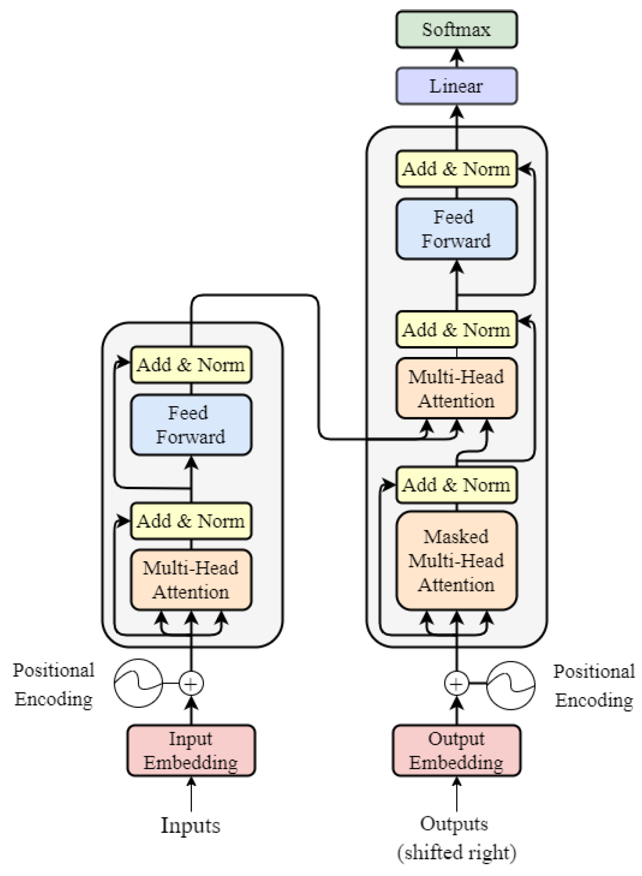
The transformer is composed of an encoder and a decoder, and its architecture is reported in Figure 1 [1]. Given such structure, there is a collection of hyperparameters needed to uniquely identify a specific architecture embodiment. The latter are reported in

Table 1. Architecture hyperparameters.

Name	Description
$vo{c}_{size}$	Number of word/tokens in the corpus
$d_{model}$	Dimension of embeddings
$d_k$	Dimension of the single attention head
$d_{ff}$	Dimension of the first layer in the feed forward network
$n_{enc}$	Number of encoder layers
$n_{dec}$	Number of decoder layers
$ma{x}_{len}$	Maximum number of tokens in the context

and they are used as parameters throughout the analysis.

5. Complexity Analysis

The method adopted for estimating the complexity of a specific learning procedure involves subdividing the latter in a series of macro-operations (e.g., forward pass, backward pass, weight update, error projection), as reported in

Table 2. Summary of the learning procedures.

Learning Methods	BP	PEP	MPE
Forward pass	1	2	3
Backward pass	1	0	0
Weight update	1	1	1
Error projection	0	1	1

PEP stands for PEPITA and MPE for MEMPEPITA.

. The total complexity of a macro-operation is obtained by calculating the complexity of performing such a macro-operation at each single layer of the transformer and adding it for all layers. In the following paragraphs, the structure and functionality of each layer is described and their complexity for the forward pass, backward pass and weight update is computed.

5.1. Embedding Layer

The embedding Layer consists of a matrix of $W_{emb}$ size $vo{c}_{size}\times d_{model}$, where each row corresponds to the embedding of a token.

5.1.1. Forward Pass

Given a sequence of N tokens, these are represented as a matrix T of size $M\times vo{c}_{size}$, where each row is a one-hot-encoded representation of the token. By multiplying the token matrix with the embedding matrix, a matrix $E=T{W}_{emb}$ of size $M\times d_{model}$ is obtained, where each row corresponds to the embedding representation of the original token in the sequence. Hence, the complexity of an embedding layer for a forward pass is, as in [11],

$$\begin{array}{|c|}\hline \mathrm{MACCs}=M\times {\mathit{voc}}_{\mathit{size}}\times d_{\mathit{model}}\\ \hline\end{array}$$

$$\begin{array}{|c|}\hline \mathrm{FLOPs}=2M\times {\mathit{voc}}_{\mathit{size}}\times d_{\mathit{model}}\\ \hline\end{array}$$

5.1.2. Weight Update (Only PEPITA and MEMPEPITA)

In BP, the gradient of the loss function with respect to the input tokens is directly calculated during the backward pass of the next layer, without involving the embedding matrix. Such gradient is directly used for updating the rows of the embedding layer corresponding to the tokens considered. Therefore, in BP no computation is needed by the embedding layer for the backward pass and weight update. On the other hand, PEPITA updates the embedding layer as for other layers, by performing a matrix multiplication. The resulting complexity of the weight update is the same as that of the forward pass.

$$\begin{array}{|c|}\hline \mathrm{MACCs}=M\times {\mathit{voc}}_{\mathit{size}}\times d_{\mathit{model}}\\ \hline\end{array}$$

$$\begin{array}{|c|}\hline \mathrm{FLOPs}=2M\times {\mathit{voc}}_{\mathit{size}}\times d_{\mathit{model}}\\ \hline\end{array}$$

5.2. Position Embeddings

A positional embedding matrix P of size $ma{x}_{len}\times d_{model}$ is used to store the positional embeddings for each position up to the maximum number of tokens in the context. To encode positional information, the first M rows of the positional matrix are added to E. The obtained matrix of size $M\times d_{model}$ is indicated with X. A positional embedding matrix can be learned or it can be already assigned following the sinusoidal positional encoding proposed in [1]. Being a simple addition operation, its complexity is negligible and can be considered to be already incorporated in the MACCs/FLOPs of the embedding layer.

5.3. Multihead Attention

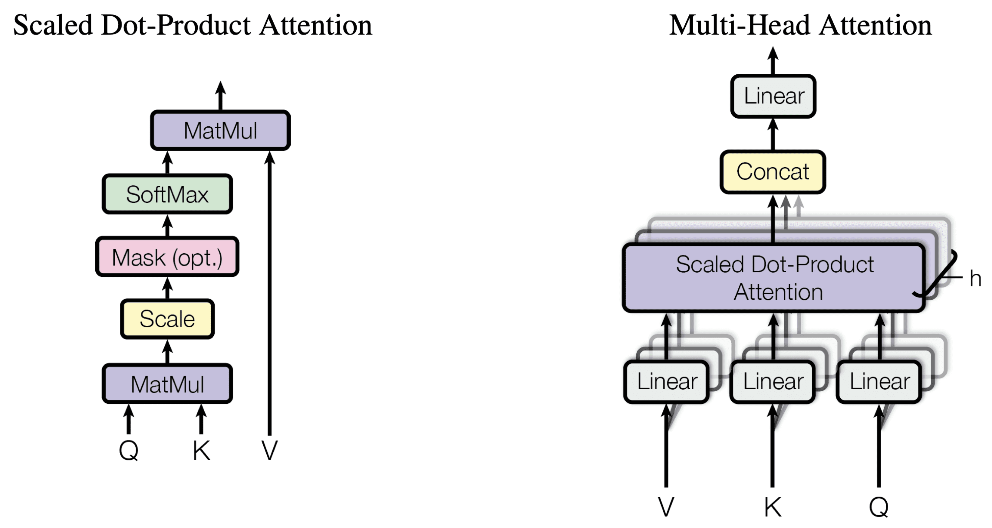
This is the most important block in the transformer, and it occupies the first stage of the encoder layer and the first two stages of the decoder layer. Its structure is reported in Figure 2 [1].

5.3.1. Forward Pass

The first step consists in identifying the input query, key and value matrices $X^Q$ of size $M\times d_{model}$ and $X^K$, $X^V$ of size $N\times d_{model}$. Then, for each different head i, $Q_i,K_i$ and $V_i$ are computed where the number of heads h is determined by dividing $d_{model}$ by $d_k$. This is achieved by multiplying the inputs with appropriate weight matrices of size $d_{model}\times d_k$.

$$(Q_i,K_i,V_i)=(X^Q{W}_i^Q,X^K{W}_i^K,X^V{W}_i^V)$$

(2)

$$\mathrm{MACCs}=M\times d_{model}\times d_{model}+2\times N\times d_{model}\times d_{model}$$

$$\mathrm{FLOPs}=2M\times d_{model}\times d_{model}+4\times N\times d_{model}\times d_{model}$$

Then, the $Q_i$, $K_i$ and $V_i$ matrices are fed into the attention mechanism of each head. It is assumed, in accordance with the conventions adopted in [11], that computing the softmax of an array of size N requires 5N FLOPs.

$$\mathrm{Attention}(Q_i,K_i,V_i)=\mathrm{softmax}\left(\frac{Q_i{K}_i^T}{\sqrt{d_k}}\right)V_i$$

(3)

$$\mathrm{MACCs}=2M\times N\times d_{model}$$

$$\mathrm{FLOPs}=4M\times N\times d_{model}+M\times 5N\times h+M\times N\times h$$

The output of the attention of each head is concatenated and multiplied by a weight matrix $W^O$ of size $d_{model}\times d_{model}$. Summing up, the output of a multihead attention block is

$$\begin{array}{c}\hfill \mathrm{Multihead}(X^Q,X^K,X^V)=\mathrm{Concat}({\mathrm{head}}_1,\dots ,{\mathrm{head}}_h)W^O\\ \hfill \mathrm{where}{\mathrm{head}}_i=\mathrm{Attention}(Q_i,K_i,V_i)\end{array}$$

(4)

$$\mathrm{MACCs}=M\times d_{model}\times d_{model}$$

$$\mathrm{FLOPs}=2M\times d_{model}\times d_{model}$$

The multihead attention block in the decoder builds the query matrix $Q_i$ starting from the output of the previous masked multihead attention block in the decoder $X_{dec}$, while the key and value matrices are obtained from the output of the encoder stack $X_{enc}$. Namely,

$$(Q_i,K_i,V_i)=(X_{dec}{W}_i^Q,X_{enc}{W}_i^K,X_{enc}{W}_i^V)$$

(5)

The masked multihead attention puts a mask on the softmax output, during training, in order for tokens not to look for a correlation with the next tokens in the sequence. The complexity of this operation is not considered, as it consists in putting to −inf certain cells of the matrix.

The total number of MACCs are

$$\begin{array}{|c|}\hline 2M\times d_{model}\times d_{model}+2M\times N\times d_{model}+2N\times d_{model}\times d_{model}\\ \hline\end{array}$$

The total number of FLOPs are

$$\begin{array}{|c|}\hline 4M\times d_{model}\times d_{model}+4M\times N\times d_{model}+4N\times d_{model}\times d_{model}+6M\times N\times h\\ \hline\end{array}$$

5.3.2. Backward Pass and Weight Update

The learnable parameters in the multiheaded attention block are the weight matrices $W_i^Q$, $W_i^K$, $W_i^V$ and $W_O$. During bakcpropagation, the derivatives of the output of the block with respect to these matrices and with respect to the inputs $X^Q,X^K$ and $X^V$ should therefore be calculated. If it is a multihead encoder or masked multihead decoder: $X^Q=X^K=X^V=X$; if it is a multihead decoder: $X^Q=X_{dec}$ and $X^K=X^V=X_{enc}$. Let us denote $f(X^Q,X^K,X^V)=\mathrm{multihead}\mathrm{attention}(X^Q,X^K,X^V)$ and indicate with $\mathcal{L}$ the loss function.

$$f=\mathrm{Concat}({\mathrm{head}}_1,\dots ,{\mathrm{head}}_h)W^O$$

(6)

$$\frac{\partial \mathcal{L}}{\partial W^O}=\mathrm{Concat}({\mathrm{head}}_1,\dots ,{\mathrm{head}}_h{)}^T\frac{\partial \mathcal{L}}{\partial f}$$

(7)

$$\frac{\partial \mathcal{L}}{\mathrm{Concat}({\mathrm{head}}_1,\dots ,{\mathrm{head}}_h)}=\frac{\partial \mathcal{L}}{\partial f}{\left(W^O\right)}^T$$

(8)

Then, the derivatives of the attention module, considering the different heads, result in the following:

$$\mathrm{Attention}(Q_i,K_i,V_i)=\mathrm{softmax}\left(\frac{Q_i{K}_i^T}{\sqrt{d_k}}\right)V_i$$

(9)

$$\frac{\partial \mathcal{L}}{\partial \mathrm{softmax}}=\frac{\partial \mathcal{L}}{\partial \mathrm{Attention}}{V}_i^T$$

(10)

Every row of the softmax is independent from the other rows. Given a row $\left[\begin{array}{ccccc}{x}_1& x_2& x_3& \cdots & x_n\end{array}\right]$ and the softmax of that row $\left[\begin{array}{ccccc}{s}_1& s_2& s_3& \cdots & s_n\end{array}\right]$ the jacobian of the softmax with respect to the row is

$$\begin{array}{c}\left[\begin{array}{ccccc}{s}_1·(1-s_1)& -s_2·s_1& -s_3·s_1& \cdots & -s_n·s_1\\ -s_1·s_2& s_2·(1-s_2)& -s_3·s_2& \cdots & -s_n·s_2\\ ⋮& ⋮& ⋮& \ddots & ⋮\\ -s_1·s_n& -s_2·s_n& -s_3·s_n& \cdots & s_n·(1-s_n)\end{array}\right]\end{array}$$

(11)

It is possible to define a 3-dimensional matrix composed of the Jacobian of each row of the softmax layer, denoted as $\frac{\partial \mathrm{softmax}}{\partial X}$, where X is a 2-dimensional matrix in $\mathrm{softmax}\left(X\right)$. In order to maintain a concise notation, we also introduce a new type of matrix product ${\times }_{slice}$ which multiplies each row of the first 2-dimensional matrix by each slice of the 3d matrix. The complexity of this product is the same as the regular matrix product.

$$\frac{\partial \mathcal{L}}{\partial Q_i{K}_i^T}=\frac{\partial \mathcal{L}}{\partial \mathit{softmax}}{\times }_{slice}{\left(\frac{\partial \mathrm{softmax}}{\partial \frac{Q_i{K}_i^T}{\sqrt{d_k}}}\right)}^T\frac{1}{\sqrt{d_k}}$$

(12)

Now, the derivative of the loss function with respect to $Q_i$, $K_i$, $V_i$ is obtained.

$$\frac{\partial \mathcal{L}}{\partial Q_i}=\frac{\partial \mathcal{L}}{\partial Q_i{K}_i^T}{K}_i$$

(13)

$$\frac{\partial \mathcal{L}}{\partial K_i}={\left(\frac{\partial \mathcal{L}}{\partial Q_i{K}_i^T}\right)}^T{Q}_i$$

(14)

$$\frac{\partial \mathcal{L}}{\partial V_i}={\mathrm{softmax}}^T\frac{\partial \mathcal{L}}{\partial \mathrm{Attention}}$$

(15)

The derivatives with respect to the inputs $X^Q$, $X^K$ and $X^V$ for each head i are the following:

$${\left(\frac{\partial \mathcal{L}}{\partial X^Q}\right)}_i=\frac{\partial \mathcal{L}}{\partial Q_i}{\left(W_i^Q\right)}^T$$

(16)

$${\left(\frac{\partial \mathcal{L}}{\partial X^K}\right)}_i=\frac{\partial \mathcal{L}}{\partial K_i}{\left(W_i^K\right)}^T$$

(17)

$${\left(\frac{\partial \mathcal{L}}{\partial X^V}\right)}_i=\frac{\partial \mathcal{L}}{\partial V_i}{\left(W_i^V\right)}^T$$

(18)

Then, the derivatives with respect to the weight matrix are computed:

$$\frac{\partial \mathcal{L}}{\partial W_i^Q}={\left(X^Q\right)}^T\frac{\partial \mathcal{L}}{\partial Q_i}$$

(19)

$$\frac{\partial \mathcal{L}}{\partial W_i^K}={\left(X^K\right)}^T\frac{\partial \mathcal{L}}{\partial K_i}$$

(20)

$$\frac{\partial \mathcal{L}}{\partial W_i^V}={\left(X^V\right)}^T\frac{\partial \mathcal{L}}{\partial V_i}$$

(21)

To obtain the derivative with respect to $X^Q$, $X^K$ and $X^V$, it is required to add all heads. As $X^Q$, $X^K$ and $X^V$ are the same for the encoder, they are all added together. In the decoder, only the derivatives with respect to $X^K$ and $X^V$ are added together as they come from the encoder. Let N be the dimension of $X^K$ and $X^V$ and M be the dimension of $X^Q$.

The complexity for each operation during the backward pass can be calculated as follows:

$$\frac{\partial \mathcal{L}}{\mathrm{Concat}({\mathrm{head}}_1,\dots ,{\mathrm{head}}_h)}=\frac{\partial \mathcal{L}}{\partial f}{\left(W^O\right)}^T$$

(22)

$$\mathrm{MACCs}=M\times d_{model}\times d_{model}$$

$$\mathrm{FLOPs}=2M\times d_{model}\times d_{model}$$

$$\frac{\partial \mathcal{L}}{\partial W^O}=\mathrm{Concat}({\mathrm{head}}_1,\dots ,{\mathrm{head}}_h{)}^T\frac{\partial \mathcal{L}}{\partial f}$$

(23)

$$\mathrm{MACCs}=d_{model}\times M\times d_{model}$$

$$\mathrm{FLOPs}=2d_{model}\times M\times d_{model}$$

In order to compute the derivative of the loss function with respect to $X^V$ and $W_i^V$, the following complexities are obtained:

$$\frac{\partial \mathcal{L}}{\partial V_i}={\mathrm{softmax}}^T\frac{\partial \mathcal{L}}{\partial {\mathrm{Attention}}_i}$$

(24)

$$\mathrm{MACCs}=N\times M\times d_k\times h=N\times M\times d_{model}$$

$$\mathrm{FLOPs}=2N\times M\times d_{model}$$

$${\left(\frac{\partial \mathcal{L}}{\partial X^V}\right)}_i=\frac{\partial \mathcal{L}}{\partial V_i}{\left(W_i^V\right)}^T$$

(25)

$$\frac{\partial \mathcal{L}}{\partial X^V}=\sum _{i=1}^h{\left(\frac{\partial \mathcal{L}}{\partial X^V}\right)}_i$$

(26)

$$\mathrm{MACCs}=N\times d_k\times d_{model}\times h=N\times d_{model}\times d_{model}$$

$$\mathrm{FLOPs}=2N\times d_{model}\times d_{model}$$

$$\frac{\partial \mathcal{L}}{\partial W_i^V}={\left(X^V\right)}^T\frac{\partial \mathcal{L}}{\partial V_i}$$

(27)

$$\mathrm{MACCs}=d_{model}\times N\times d_k\times h=d_{model}\times N\times d_{model}$$

$$\mathrm{FLOPs}=2d_{model}\times N\times d_{model}$$

In order to compute the derivative of the loss function with respect to $X^Q$, $X^K$, $W_i^Q$ and $W_i^K$, the following complexities are obtained:

$$\frac{\partial \mathrm{softmax}}{\partial \frac{Q_i{K}_i^T}{\sqrt{d_k}}}$$

(28)

$$\mathrm{MACCs}=0$$

$$\mathrm{FLOPs}=N\times N\times M\times h$$

$$\frac{\partial \mathcal{L}}{\partial Q_i{K}_i^T}=\frac{\partial \mathcal{L}}{\partial \mathrm{Attention}}{V}_i^T{\times }_{slice}{\left(\frac{\partial \mathrm{softmax}}{\partial \frac{Q_i{K}_i^T}{\sqrt{d_k}}}\right)}^T\frac{1}{\sqrt{d_k}}$$

(29)

$$\mathrm{MACCs}=M\times d_{model}\times N+M\times N\times M\times h$$

$$\mathrm{FLOPs}=2M\times d_{model}\times N+2M\times N\times M\times h+M\times N\times h$$

$$\frac{\partial \mathcal{L}}{\partial Q_i}=\frac{\partial \mathcal{L}}{{\partial Q_i{K}_i}^T}{K}_i$$

(30)

$$\mathrm{MACCs}=M\times N\times d_{model}$$

$$\mathrm{FLOPs}=2M\times N\times d_{model}$$

$${\left(\frac{\partial \mathcal{L}}{\partial X^Q}\right)}_i=\frac{\partial \mathcal{L}}{\partial Q_i}{\left(W_i^Q\right)}^T$$

(31)

$$\frac{\partial \mathcal{L}}{\partial X^Q}=\sum _{i=1}^h{\left(\frac{\partial \mathcal{L}}{\partial X^Q}\right)}_i$$

(32)

$$\mathrm{MACCs}=M\times d_{model}\times d_{model}$$

$$\mathrm{FLOPs}=2M\times d_{model}\times d_{model}$$

$$\frac{\partial \mathcal{L}}{\partial W_i^Q}={\left(X^Q\right)}^T\frac{\partial \mathcal{L}}{\partial Q_i}$$

(33)

$$\mathrm{MACCs}=d_{model}\times M\times d_{model}$$

$$\mathrm{FLOPs}=2d_{model}\times M\times d_{model}$$

$$\frac{\partial \mathcal{L}}{\partial K_i}={\left(\frac{\partial \mathcal{L}}{{\partial Q_i{K}_i}^T}\right)}^T{Q}_i$$

(34)

$$\mathrm{MACCs}=N\times M\times d_{model}$$

$$\mathrm{FLOPs}=2N\times M\times d_{model}$$

$${\left(\frac{\partial \mathcal{L}}{\partial X^K}\right)}_i=\frac{\partial \mathcal{L}}{\partial K_i}{\left(W_i^K\right)}^T$$

(35)

$$\frac{\partial \mathcal{L}}{\partial X^K}=\sum _{i=1}^h{\left(\frac{\partial \mathcal{L}}{\partial X^K}\right)}_i$$

(36)

$$\mathrm{MACCs}=N\times d_{model}\times d_{model}$$

$$\mathrm{FLOPs}=2N\times d_{model}\times d_{model}$$

$$\frac{\partial \mathcal{L}}{\partial W_i^K}={\left(X^K\right)}^T\frac{\partial \mathcal{L}}{\partial K_i}$$

(37)

$$\mathrm{MACCs}=d_{model}\times N\times d_{model}$$

$$\mathrm{FLOPs}=2d_{model}\times N\times d_{model}$$

In the case of the multihead attention encoder and of the masked multihead attention decoder, it should be considered that $X^Q=X^K=X^V$ ( $M=N$ ), and the derivatives with respect to $X^Q$, $X^K$ and $X^V$ are added. Conversely, in the multi-head attention decoder, it holds that $X^Q\ne X^K=X^V$ (M ≠ N), and only the derivatives with respect to $X^K$ and $X^V$ are added. The complexity of these operations is marginal and can be considered to be already integrated in previous MACCs/FLOPs.

In conclusion, the backward pass has a complexity of

$$\begin{array}{|c|}\hline \mathrm{MACCs}=\\ 2M\times d_{model}\times d_{model}+2N\times d_{model}\times d_{model}+4M\times N\times d_{model}+M\times N\times M\times h\\ \hline\end{array}$$

$$\begin{array}{|c|}\hline \mathrm{FLOPs}=4M\times d_{model}\times d_{model}+4N\times d_{model}\times d_{model}+8M\times N\times d_{model}+2M\times N \times \\ M\times h+M\times N\times h\\ \hline\end{array}$$

and the weight update has a complexity of

$$\begin{array}{|c|}\hline \mathrm{MACCs}=2M\times d_{model}\times d_{model}+2N\times d_{model}\times d_{model}\\ \hline\end{array}$$

$$\begin{array}{|c|}\hline \mathrm{FLOPs}=4M\times d_{model}\times d_{model}+4N\times d_{model}\times d_{model}\\ \hline\end{array}$$

5.4. Feed-Forward Network

The feed-forward network (FFN) is a 2-layer neural network, where the first layer is of size $M\times d_{ff}$ and the second $M\times d_{model}$. Only the first layer uses an activation function.

$$\mathrm{FFN}\left(x\right)=\mathrm{GELU}(x{W}_1+b_1)W_2+b_2$$

(38)

5.4.1. Forward Pass

$$\begin{array}{|c|}\hline \mathrm{MACCs}=2M\times d_{model}\times d_{\mathit{ff}}\\ \hline\end{array}$$

The FLOPs for the GeLU activation are assumed to be 8 FLOPs in the forward pass and 13 FLOPs for computing the derivative.

The FLOPs accounting for bias and NL are

$$\begin{array}{|c|}\hline \mathrm{FLOPs}=4M\times d_{model}\times d_{\mathit{ff}}+9M\times d_{\mathit{ff}}+M\times d_{model}\\ \hline\end{array}$$

5.4.2. Backward Pass

The backward pass is characterized by the following complexity.

$$\begin{array}{|c|}\hline \mathrm{MACCs}=2M\times d_{\mathit{ff}}\times d_{model}\\ \hline\end{array}$$

$$\begin{array}{|c|}\hline \mathrm{FLOPs}=4M\times d_{model}\times d_{\mathit{ff}}+13M\times d_{\mathit{ff}}\\ \hline\end{array}$$

5.4.3. Weight Update

The weight update requires the following complexity.

$$\begin{array}{|c|}\hline \mathrm{MACCs}=2M\times d_{\mathit{ff}}\times d_{model}\\ \hline\end{array}$$

$$\begin{array}{|c|}\hline \mathrm{FLOPs}=4M\times d_{\mathit{ff}}\times d_{model}\\ \hline\end{array}$$

5.5. Add and Norm

After each multihead attention and feed-forward block, the input to the block, indicated as sublayer, is added, and a layer normalization is applied.

$$\mathrm{LayerNorm}(x+\mathrm{Sublayer}(x\left)\right)$$

(39)

Layer The normalization normalizes the features across each token, multiplies the results by $\gamma$ and adds $\beta$, where $\gamma$ and $\beta$ are learnable parameters.

$$\mathrm{LayerNorm}\left(x\right)=\frac{x-E\left[x\right]}{\sqrt{\mathrm{Var}\left[x\right]}}\gamma +\beta$$

(40)

5.5.1. Forward Pass

Such operation does not properly constitute a MACC.

$$\mathrm{MACCs}=0$$

Operations that are performed for each neuron are considered. The square root is only performed once. The other operations are addition for the mean, subtract, square and addition for the variance, subtract, divide, bias (add) and scale (multiply). It results in 8 FLOPs per neuron. Furthermore, the FLOPs relative to the addition between x and the sublayer should also be considered:

$$\begin{array}{|c|}\hline \mathrm{MACCs}=0\\ \hline\end{array}$$

$$\begin{array}{|c|}\hline \mathrm{FLOPs}=9M\times d_{model}\\ \hline\end{array}$$

5.5.2. Backward Pass and Weight Update

To train the parameters $\gamma$ and $\beta$, we first need to compute the derivative of layernorm. The layer-normalized activation matrix is denoted as z.

$$\frac{\partial \mathcal{L}}{\partial {\gamma }_j}=\sum _i^M\frac{\partial \mathcal{L}}{\partial {\mathrm{Layernorm}}_{ij}}{z}_{ij}$$

(41)

$$\mathrm{MACCs}=M\times d_{model}$$

$$\mathrm{FLOPs}=2M\times d_{model}$$

$$\frac{\partial \mathcal{L}}{\partial {\beta }_j}=\sum _i^M\frac{\partial \mathcal{L}}{\partial {\mathrm{Layernorm}}_{ij}}$$

(42)

$$\mathrm{MACCs}=0$$

$$\mathrm{FLOPs}=M\times d_{model}$$

$$\frac{\partial \mathcal{L}}{\partial z_{ij}}=\frac{\partial \mathcal{L}}{\partial {\mathrm{Layernorm}}_{ij}}{\gamma }_{ij}$$

(43)

$$\mathrm{MACCs}=0$$

$$\mathrm{FLOPs}=M\times d_{model}$$

The Jacobian of activation vector $z_i$ with respect to $x_i$ is defined as $ja{c}_i={\{\frac{\partial z_{ij}}{\partial x_{ik}}=\frac{1}{\sigma }({\delta }_{jk}-\frac{1}{d_{model}}-\frac{(x_j-\mu )(x_k-\mu )}{d_{model}{\sigma }^2})\}}_{jk}$. By combining the various Jacobians for each row $z_i$, a 3d matrix $jac$ is obtained, where each slice corresponds to the Jacobian of a row vector. The operations involved in such a computation do not properly constitute MACCs. The FLOPs to calculate the Jacobian is 3 muls, 2 divisions, 4 adds, namely 9 FLOPs for each element.

$$\mathrm{MACCs}=0$$

$$\mathrm{FLOPs}=9\times M\times d_{model}\times d_{model}$$

To obtain the derivative

$$\frac{\partial \mathcal{L}}{\partial X}=\frac{\partial \mathcal{L}}{\partial z}{\times }_{slice}jac$$

(44)

$$\mathrm{MACCs}=M\times d_{model}\times d_{model}$$

$$\mathrm{FLOPs}=2M\times d_{model}\times d_{model}$$

Then, FLOPs used to add the derivative for the skip layer should also be taken into account.

$$\mathrm{MACCs}=0$$

$$\mathrm{MACCs}=M\times d_{model}$$

The total number of MACCs for backward are

$$\begin{array}{|c|}\hline \mathrm{MACCs}=M\times d_{model}\times d_{model}\\ \hline\end{array}$$

$$\begin{array}{|c|}\hline \mathrm{FLOPs}=11M\times d_{model}\times d_{model}+2M\times d_{model}\\ \hline\end{array}$$

The total number of MACCs for weight update are

$$\begin{array}{|c|}\hline \mathrm{MACCs}=M\times d_{model}\\ \hline\end{array}$$

$$\begin{array}{|c|}\hline \mathrm{FLOPs}=3M\times d_{model}\\ \hline\end{array}$$

5.6. Softmax Layer

At the end of the transformer, there is a softmax layer where the weight matrix $W^S$ is of size $d_{model}\times vo{c}_{size}$.

$$\mathrm{Softmax}\left(X{W}^S\right)$$

(45)

5.6.1. Forward Pass

The forward pass requires

$$\begin{array}{|c|}\hline \mathrm{MACCs}=M\times d_{model}\times {\mathit{voc}}_{\mathit{size}}\\ \hline\end{array}$$

The softmax function requires 5N FLOPs for an array of N elements. Hence, the number of FLOPs are

$$\begin{array}{|c|}\hline \mathrm{FLOPs}=2M\times d_{model}\times {\mathit{voc}}_{\mathit{size}}+M\times 5{\mathit{voc}}_{\mathit{size}}\\ \hline\end{array}$$

5.6.2. Backward Pass and Weight Update

The derivative of the loss with respect to Z, with Z being the product of X with W^s is $\frac{\partial \mathcal{L}}{\partial z}=target-s$. As the target is usually a one hot encoded vector, it is assumed that such operation has no FLOPs or MACCs.

$$\frac{\partial \mathcal{L}}{\partial X}=\frac{\partial \mathcal{L}}{\partial Z}{\left(W^S\right)}^T$$

(46)

$$\mathrm{MACCs}=M\times vo{c}_{size}\times d_{model}$$

$$\mathrm{FLOPs}=2M\times vo{c}_{size}\times d_{model}$$

$$\frac{\partial \mathcal{L}}{\partial W^S}=X^T\frac{\partial \mathcal{L}}{\partial Z}$$

(47)

$$\mathrm{MACCs}=d_{model}\times M\times vo{c}_{size}$$

$$\mathrm{FLOPs}=2d_{model}\times M\times vo{c}_{size}$$

The total number of MACCs for backward are

$$\begin{array}{|c|}\hline \mathrm{MACCs}=M\times {\mathit{voc}}_{\mathit{size}}\times d_{model}\\ \hline\end{array}$$

$$\begin{array}{|c|}\hline \mathrm{FLOPs}=2M\times {\mathit{voc}}_{\mathit{size}}\times d_{model}\\ \hline\end{array}$$

The total number of MACCs for weight update are

$$\begin{array}{|c|}\hline \mathrm{MACCs}=d_{model}\times M\times {\mathit{voc}}_{\mathit{size}}\\ \hline\end{array}$$

$$\begin{array}{|c|}\hline \mathrm{FLOPs}=2d_{model}\times M\times {\mathit{voc}}_{\mathit{size}}\\ \hline\end{array}$$

5.7. Error Projection (Only PEPITA and MEMPEPITA)

The output error has dimensionality $M\times vo{c}_{size}$, which is the same dimensionality as the decoder input. Therefore, a projection matrix to project it to the decoder input is not needed. On the other hand, an attention mechanism is used to project the error of dimensionality $M\times d_{model}$ to the dimensionality of the input to the encoder $N\times d_{model}$.

$$T_{err}^{enc}=Attention(T^{enc},T_{err}^{dec},T_{err}^{dec})$$

(48)

$$\begin{array}{|c|}\hline \mathrm{MACCs}=2N\times M\times {\mathit{voc}}_{\mathit{size}}\\ \hline\end{array}$$

$$\begin{array}{|c|}\hline \mathrm{FLOPs}=4N\times M\times {\mathit{voc}}_{\mathit{size}}+6N\times M\\ \hline\end{array}$$

6. Exemplary Application

To explain better the applicability of the proposed mathematical formulation, the complexity estimation in terms of MACCs for a one-block encoder-only simplified architecture trained with BP, PEPITA or MEMPEPITA is reported in this section. The layers involved in the architecture are the following (sections): embedding layer (Section 5.1), multihead attention (Section 5.3), add and norm (Section 5.5), feed-forward network (Section 5.4) and softmax (Section 5.6). To compute the number of MACCs required for a forward pass, its complexity at each layer is added together.

$$\begin{array}{|c|}\hline {\mathrm{MACCs}}_{forward}=M\times vo{c}_{size}\times d_{model}+2M\times d_{model}^2+2M\times N\times d_{model}+2N \times \\ d_{model}^2+0+2M\times d_{model}\times d_{ff}+0+M\times d_{model}\times vo{c}_{size}\\ \hline\end{array}$$

Analogously, the total number of MACCs for the backward pass and the weight update are the following:

$$\begin{array}{|c|}\hline {\mathrm{MACCs}}_{backward}=\\ 0+2M\times d_{model}\times d_{model}+2N\times d_{model}\times d_{model}+4M\times N\times d_{model}+M\times N\times M\times h +\\ M\times d_{model}\times d_{model}+2M\times d_{model}\times d_{ff}+M\times d_{model}\times d_{model}+d_{model}\times M\times vo{c}_{size}\\ \hline\end{array}$$

$$\begin{array}{|c|}\hline {\mathrm{MACCs}}_{weight-update}=M\times vo{c}_{size}\times d_{model}+2M\times d_{model}^2+2N\times d_{model}^2+M \times \\ d_{model}+2M\times d_{model}\times d_{ff}+M\times d_{model}+M\times vo{c}_{size}\times d_{model}\\ \hline\end{array}$$

The first term of the sum in the weight-update MACC estimation shall be discarded when considering BP. As the output dimension is the same as the input dimension for an encoder-only architecture, the error projections for PEPITA and MEMPEPITA are not required. Referring to Table 2, the total numbers of MACCs for training a one-block encoder-only transformer and adopting the different learning procedures are the following:

$$\begin{array}{|c|}\hline {\mathrm{MACCs}}_{\mathit{BP}}={\mathrm{MACCs}}_{\mathit{forward}}+{\mathrm{MACCs}}_{\mathit{backward}}+{\mathrm{MACCs}}_{\mathit{weight}-\mathit{update}}\\ \hline\end{array}$$

$$\begin{array}{|c|}\hline {\mathrm{MACCs}}_{\mathit{PEPITA}}=2{\mathrm{MACCs}}_{\mathit{forward}}+{\mathrm{MACCs}}_{\mathit{weight}-\mathit{update}}\\ \hline\end{array}$$

$$\begin{array}{|c|}\hline {\mathrm{MACCs}}_{\mathit{MEMPEPITA}}=3{\mathrm{MACCs}}_{\mathit{forward}}+{\mathrm{MACCs}}_{\mathit{weight}-\mathit{update}}\\ \hline\end{array}$$

7. Conclusions

In this work, the equations behind BP (reverse-mode autodiff), PEPITA and MEMPEPITA for the layers of a generic transformer architecture were derived and described. The computational complexity of the forward pass, backward pass and weight update were expressed in terms of MACCs and FLOPs for each layer, using the mathematical formulas previously obtained. An examplary application for the computation of the complexity in the case of a one-block encoder-only transformer was also reported for illustration purposes. The method proposed in this work combines the advantages of being device-agnostic with mathematical rigour, providing a robust estimation of complexity independent of the specific target. By taking advantage of the results of this paper, the reader can easily provide a reliable estimation of the computational complexity involved in training a transformer architecture of their choice using BP and forward learning procedures.

References

- Vaswani, A.; Shazeer, N.; Parmar, N.; Uszkoreit, J.; Jones, L.; Gomez, A.N.; Kaiser, L.; Polosukhin, I. Attention is All you Need. In Proceedings of the Advances in Neural Information Processing Systems, Long Beach, CA, USA, 4–9 December 2017; Curran Associates, Inc.: New York, NY, USA, 2017; Volume 30. [Google Scholar]
- Kaplan, J.; McCandlish, S.; Henighan, T.; Brown, T.B.; Chess, B.; Child, R.; Gray, S.; Radford, A.; Wu, J.; Amodei, D. Scaling Laws for Neural Language Models. arXiv 2020, arXiv:2001.08361. [Google Scholar]
- Brown, T.B.; Mann, B.; Ryder, N.; Subbiah, M.; Kaplan, J.; Dhariwal, P.; Neelakantan, A.; Shyam, P.; Sastry, G.; Askell, A.; et al. Language Models are Few-Shot Learners. arXiv 2020, arXiv:2005.14165. [Google Scholar]
- Mielke, S.J.; Alyafeai, Z.; Salesky, E.; Raffel, C.; Dey, M.; Gallé, M.; Raja, A.; Si, C.; Lee, W.Y.; Sagot, B.; et al. Between words and characters: A Brief History of Open-Vocabulary Modeling and Tokenization in NLP. arXiv 2021, arXiv:2112.10508. [Google Scholar]
- Maslej, N.; Fattorini, L.; Brynjolfsson, E.; Etchemendy, J.; Ligett, K.; Lyons, T.; Manyika, J.; Ngo, H.; Niebles, J.C.; Parli, V.; et al. The AI Index 2023 Annual Report; Technical report; AI Index Steering Committee, Institute for Human-Centered AI, Stanford University: Stanford, CA, USA, 2023. [Google Scholar]
- Hinton, G. The Forward-Forward Algorithm: Some Preliminary Investigations. arXiv 2022, arXiv:2212.13345. [Google Scholar]
- Dellaferrera, G.; Kreiman, G. Error-driven Input Modulation: Solving the Credit Assignment Problem without a Backward Pass. arXiv 2022, arXiv:2201.11665. [Google Scholar]
- Abadi, M.; Agarwal, A.; Barham, P.; Brevdo, E.; Chen, Z.; Citro, C.; Corrado, G.S.; Davis, A.; Dean, J.; Devin, M.; et al. TensorFlow: Large-Scale Machine Learning on Heterogeneous Distributed Systems. arXiv 2016, arXiv:1603.04467. [Google Scholar]
- Paszke, A.; Gross, S.; Massa, F.; Lerer, A.; Bradbury, J.; Chanan, G.; Killeen, T.; Lin, Z.; Gimelshein, N.; Antiga, L.; et al. PyTorch: An Imperative Style, High-Performance Deep Learning Library. arXiv 2019, arXiv:1912.01703. [Google Scholar]
- Baydin, A.G.; Pearlmutter, B.A.; Radul, A.A.; Siskind, J.M. Automatic Differentiation in Machine Learning: A Survey. J. Mach. Learn. Res. 2017, 18, 5595–5637. [Google Scholar]
- Clark, K.; Luong, M.T.; Le, Q.V.; Manning, C.D. Pre-Training Transformers as Energy-Based Cloze Models. In Proceedings of the EMNLP, Online, 16–20 November 2020. [Google Scholar]
- Crick, F. The recent excitement about neural networks. Nature 1989, 337, 129–132. [Google Scholar] [CrossRef]
- Lillicrap, T.; Santoro, A.; Marris, L.; Akerman, C.; Hinton, G. Backpropagation and the brain. Nat. Rev. Neurosci. 2020, 21, 335–346. [Google Scholar] [CrossRef]
- Burbank, K.S.; Kreiman, G. Depression-Biased Reverse Plasticity Rule Is Required for Stable Learning at Top-Down Connections. PLoS Comput. Biol. 2012, 8, e1002393. [Google Scholar] [CrossRef] [PubMed]
- Liao, Q.; Leibo, J.Z.; Poggio, T. How Important is Weight Symmetry in Backpropagation? arXiv 2016, arXiv:1510.05067. [Google Scholar] [CrossRef]
- Baldi, P.; Sadowski, P. A theory of local learning, the learning channel, and the optimality of backpropagation. Neural Netw. 2016, 83, 51–74. [Google Scholar] [CrossRef] [PubMed]
- Jaderberg, M.; Czarnecki, W.M.; Osindero, S.; Vinyals, O.; Graves, A.; Silver, D.; Kavukcuoglu, K. Decoupled Neural Interfaces using Synthetic Gradients. In Proceedings of the 34th International Conference on Machine Learning, Sydney, Australia, 6–11 August 2017; Volume 70, pp. 1627–1635. [Google Scholar]
- Czarnecki, W.M.; Świrszcz, G.; Jaderberg, M.; Osindero, S.; Vinyals, O.; Kavukcuoglu, K. Understanding Synthetic Gradients and Decoupled Neural Interfaces. In Proceedings of the 34th International Conference on Machine Learning, Sydney, Australia, 6–11 August 2017; Volume 70, pp. 904–912. [Google Scholar]
- Xiao, W.; Chen, H.; Liao, Q.; Poggio, T. Biologically-plausible learning algorithms can scale to large datasets. arXiv 2018, arXiv:1811.03567. [Google Scholar]
- Lillicrap, T.; Cownden, D.; Tweed, D.; Akerman, C. Random synaptic feedback weights support error backpropagation for deep learning. Nat. Commun. 2016, 7, 13276. [Google Scholar] [CrossRef] [PubMed]
- Nøkland, A. Direct Feedback Alignment Provides Learning in Deep Neural Networks. In Proceedings of the 30th International Conference on Neural Information Processing Systems, NIPS’16, Barcelona, Spain, 5–10 December 2016; pp. 1045–1053. [Google Scholar]
- Akrout, M.; Wilson, C.; Humphreys, P.; Lillicrap, T.; Tweed, D.B. Deep Learning without Weight Transport. In Proceedings of the Advances in Neural Information Processing Systems, Vancouver, BC, Canada, 8–14 December 2019; Curran Associates, Inc.: New York, NY, USA, 2019; Volume 32. [Google Scholar]
- Frenkel, C.; Lefebvre, M.; Bol, D. Learning Without Feedback: Fixed Random Learning Signals Allow for Feedforward Training of Deep Neural Networks. Front. Neurosci. 2021, 15, 629892. [Google Scholar] [CrossRef] [PubMed]
- Xie, X.; Seung, H. Equivalence of Backpropagation and Contrastive Hebbian Learning in a Layered Network. Neural Comput. 2003, 15, 441–454. [Google Scholar] [CrossRef] [PubMed]
- Scellier, B.; Bengio, Y. Equilibrium Propagation: Bridging the Gap between Energy-Based Models and Backpropagation. Front. Comput. Neurosci. 2017, 11, 24. [Google Scholar] [CrossRef]
- Clark, D.; Abbott, L.; Chung, S. Credit Assignment Through Broadcasting a Global Error Vector. In Proceedings of the Advances in Neural Information Processing Systems 34—35th Conference on Neural Information Processing Systems, NeurIPS 2021, Virtual, 6–14 December 2021; pp. 10053–10066. [Google Scholar]
- Pau, D.P.; Aymone, F.M. Suitability of Forward-Forward and PEPITA Learning to MLCommons-Tiny benchmarks. In Proceedings of the 2023 IEEE International Conference on Omni-layer Intelligent Systems (COINS), Berlin, Germany, 23–25 July 2023; pp. 1–6. [Google Scholar] [CrossRef]
- Banbury, C.; Reddi, V.J.; Torelli, P.; Holleman, J.; Jeffries, N.; Kiraly, C.; Montino, P.; Kanter, D.; Ahmed, S.; Pau, D.; et al. MLCommons Tiny Benchmark. In Proceedings of the Neural Information Processing Systems Track on Datasets and Benchmarks, Virtual, 6–14 December 2021. [Google Scholar]
- Srinivasan, R.F.; Mignacco, F.; Sorbaro, M.; Refinetti, M.; Cooper, A.; Kreiman, G.; Dellaferrera, G. Forward Learning with Top-Down Feedback: Empirical and Analytical Characterization. arXiv 2023, arXiv:2302.05440. [Google Scholar]
- Justus, D.; Brennan, J.; Bonner, S.; McGough, A.S. Predicting the Computational Cost of Deep Learning Models. arXiv 2018, arXiv:1811.11880. [Google Scholar]
- Zargar, B.; Ponci, F.; Monti, A. Evaluation of Computational Complexity for Distribution Systems State Estimation. IEEE Trans. Instrum. Meas. 2023, 72, 9001512. [Google Scholar] [CrossRef]
- Muhammad, N.; Bibi, N.; Jahangir, A.; Mahmood, Z. Image denoising with norm weighted fusion estimators. Form. Pattern Anal. Appl. 2018, 21, 1013–1022. [Google Scholar] [CrossRef]
- Getzner, J.; Charpentier, B.; Günnemann, S. Accuracy is not the only Metric that matters: Estimating the Energy Consumption of Deep Learning Models. arXiv 2023, arXiv:2304.00897. [Google Scholar]
Disclaimer/Publisher’s Note: The statements, opinions and data contained in all publications are solely those of the individual author(s) and contributor(s) and not of MDPI and/or the editor(s). MDPI and/or the editor(s) disclaim responsibility for any injury to people or property resulting from any ideas, methods, instructions or products referred to in the content. |
© 2023 by the authors. Licensee MDPI, Basel, Switzerland. This article is an open access article distributed under the terms and conditions of the Creative Commons Attribution (CC BY) license (https://creativecommons.org/licenses/by/4.0/).